國 立 交 通 大 學
電控工程研究所
碩 士 論 文
使用加速規之慣性滑鼠裝置訊號處理方法評估
Evaluations of Signal Processing Methods for an Inertial
Mouse Device Using Accelerometers
研 究 生: 活 多 福
指導教授: 胡 竹 生 博士
使用加速規之慣性滑鼠裝置訊號處理方法評估
研究生:活 多 福
指導教授:胡 竹 生 博士
國立交通大學
電控工程研究所碩士班
摘要
本論文提出了一個以三軸加速度計來取代普遍用於商業滑鼠裝置的光學感 測器的新型慣性滑鼠裝置。本 論文所使用的慣性感測器為加速度計,其具有減 少能量耗損、縮減整體產品大小以及減低整體產品成本的優點,另外因為此種新 型的 慣性滑鼠裝置可以隔空使用,所以也增加了其可使用的範圍。本論文以光學感應器及三軸加速度計來實現所提出的 慣性滑鼠裝置,因此 能在相同環境及條件下比較兩種不同感應器﹝光學感應器及慣性感應器 ﹞的效 果。本論文以不同的數學方法以及從加速度計所得到的訊號來估測滑鼠裝置的位 移量。 在最初時,這些實現的演算法皆以個人電腦為核心並搭配慣性滑鼠裝置 來做測試,最後最適合的演算法則以微控制器來實現,整個 裝置成為一個獨立 的新型慣性滑鼠裝置。 實 驗結果顯示出,本論文所提出的以加速度計為基礎的最佳估測技術可 以 做為新型的慣性滑鼠裝置,且應用在一般的電腦上可以順利完成大多數的工作。
Evaluations of Signal Processing Methods for an Inertial
Mouse Device Using Accelerometers
Student: Rodolfo Gondim Lóssio
Advisor: Prof. Jwu-Sheng Hu
Institute of Electrical and Control Engineering
National Chiao-Tung University
ABSTRACT
This work proposes and evaluates an inertial mouse device based on three-axis accelerometer to be a substitute of the optical sensor, which is commonly used in the majority of commercial mouse devices. The use of inertial sensors, such as accelerometers, will allow reducing power consumption, physical dimensions and final product cost, moreover will increase easy-of-use, since this kind of mouse could be also used in free space.
For this purpose, a prototype containing an optical sensor and 3-axis accelerometer is built. In this way, it is possible to compare the two sensors under the same environment and conditions. In a first moment, different mathematical approaches are tested to estimate the displacement based on the acceleration signal. Those approaches are processed under a computer application connected to the prototype. By the end, the most suitable algorithms are ported to the microcontroller embedded in the prototype.
The result of the experiments show that the best estimator techniques based on the accelerometers can be used as a mouse device to perform the majority of the tasks when interacting with a computer.
Acknowledgments
My first words will go to my family in Brazil, which will be written in Portuguese:
“Aos meus pais e irmãos, gostaria de agradeçe-los por todo o suporte que vocês me deram durante esses dois anos e pouco que estive no exterior estudando e trabalhando. Sem esse suporte, acredito que não conseguiria ir tão longe nos meus estudos e na minha vida profissional. Sinto muita falta de vocês e gostaria muito que vocês estivessem na minha cerimônia de graduação. Mas por causa da distância, tempo e dinheiro, esse desejo torna-se quase impossível. Mesmo assim, espero que no futuro vocês possam conhecer esse país que me conquistou e deu enorme oportunidades para meu crescimento profissional e acadêmico.”
For the people from Taiwan, at first I would like to thank my advisor, Prof. Hu, for accepting to orientate my research for these two years. It was a pleasure for me to have worked together with such a really competent and qualified professor.
Also, I would like to thank my labmates from X-Lab, who helped me a lot, specially with the bureaucratic stuff that concerns with the academic life. I made really good friends in here, and I hope we can keep in touch for a long time.
And for last, I would like to thank my girlfriend, Charlene, for helping me since my first month in Taiwan. It is not easy to stay far away from family. But with her help, I overcome this problem, and she is one of the main reasons I feel at home in Taiwan now.
Contents
摘要 ... i
ABSTRACT ... iii
Acknowledgments ... iv
Contents ... v
List of Tables ... vii
List of Figures ... viii
Chapter 1. Introduction ... 1
1.1 MOTIVATION AND OBJECTIVE ... 1
1.2 SURVEY OF PREVIOUS WORK ... 2
1.3 THESIS SUBJECT AND CONTRIBUTION ... 3
1.4 OUTLINES OF THESIS ... 4
Chapter 2. The Prototype... 6
2.1 THE COMPONENTS ... 6
2.1.1 Microcontroller ... 6
2.1.2 Three-Axis Accelerometer ... 7
2.1.3 Optical Sensor ... 7
2.2 THE LAYOUT AND PHYSICAL STRUCTURE ... 8
2.3 SOFTWARE DEVELOPMENT ... 9
2.3.1 USB Drivers and Device Classes ... 9
2.3.2 Host Application ... 11
2.3.3 Embedded Application ... 14
Chapter 3. Signal Processing Methods ... 17
3.1 DATA PREPARATION ... 17
3.1.1 Statistical Techniques ... 17
3.1.2 Bias filtering ... 18
3.1.3 Calibration Process ... 23
3.2 THE FUZZY-NEURAL INTEGRATOR ... 25
3.2.1 Membership functions ... 27
3.2.2 Fuzzy Rules ... 29
3.2.4 Back Propagation Algorithm ... 30
3.2.5 Fuzzy-Neural Model ... 33
3.3 THE KALMAN FILTER... 37
3.3.1 The Process to be estimated ... 38
3.3.2 Filter Parameters and Tuning ... 39
3.4 THE STATE-MACHINE ESTIMATOR ... 41
3.4.1 State-Machine using simple integration method ... 42
3.4.2 State-Machine using Kalman filter ... 46
3.4.3 Combined Axis XY State-Machine ... 48
3.4.4 Combined State-Machine using motion detection sensor... 52
3.4.5 Combined State-Machine using physical button ... 53
3.4.6 State-Machine using inertial behavior ... 53
Chapter 4. Testing and Experimental Results ... 58
4.1 ANALYTICAL RESULTS ... 58
4.1.1 Graphical Results ... 58
4.1.2 Mathematical Results ... 67
4.2 THE TEST SCENARIO ... 69
4.3 PERFORMANCE RESULTS... 71
Chapter 5. Conclusions and Future Work ... 77
List of Tables
TABLE 1:BINARY PACKET SENT BY THE PROTOTYPE ... 12
TABLE 2:FUZZY-NEURAL NETWORK TABLE (FIRST VERSION) ... 34
TABLE 3:STATES, TRANSITIONS AND ACTIONS OF THE STATE-MACHINE USING SIMPLE INTEGRATION ... 45
TABLE 4:STATES, TRANSITIONS AND ACTIONS OF THE STATE-MACHINE USING KALMAN FILTER ... 47
TABLE 5:STATES, TRANSITIONS AND ACTIONS OF THE COMBINED STATE-MACHINE ... 51
TABLE 6:STATES, TRANSITIONS AND ACTIONS OF THE FREE MOVEMENT STATE-MACHINE ... 57
TABLE 7:MATHEMATICAL ANALYSIS IN HIGH SPEED SCENARIO ... 68
TABLE 8:MATHEMATICAL ANALYSIS IN LOW SPEED SCENARIO ... 68
List of Figures
FIGURE 1:CROSS SECTION OF A PCB ASSEMBLY ... 8
FIGURE 2:PROTOTYPE'S LAYOUT ... 9
FIGURE 3:HIERARCHY FROM SOFTWARE APPLICATION TO USB DEVICE ... 10
FIGURE 4:SAMPLING TIME LINE ... 15
FIGURE 5:FLOW CHART FROM THE EMBEDDED APPLICATION ... 16
FIGURE 6:RAW ACCELERATION FROM ZAXIS (NO SCALE) ... 18
FIGURE 7:RAW ACCELERATION OF XYZ AXES WITHOUT MOVING THE PROTOTYPE ... 19
FIGURE 8:AFTER CONSTANT BIAS COMPENSATION ... 20
FIGURE 9:UNBIASED ACCELERATION AFTER APPLYING FILTER H(Z) WITH DIFFERENT : ... 21
FIGURE 10:CLOSER LOOK IN THE END OF THE MOVEMENT ... 22
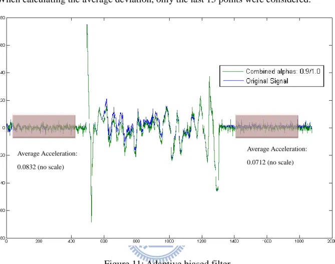
FIGURE 11:ADAPTIVE BIASED FILTER... 23
FIGURE 12:CONFIGURATION OF THE FUZZY NEURAL NETWORK ... 26
FIGURE 13:ACCELERATION MEMBERSHIP FUNCTION ... 28
FIGURE 14:VELOCITY MEMBERSHIP FUNCTION ... 29
FIGURE 16:BLOCK DIAGRAM FROM COLLECTING PHASE ... 31
FIGURE 17:BLOCK DIAGRAM FROM TRAINING PHASE ... 32
FIGURE 18:DIAGRAM BLOCK FROM VALIDATION PHASE ... 33
FIGURE 19:MODIFIED FUZZY-NEURAL NETWORK ... 36
FIGURE 20:THE DISCRETE KALMAN FILTER CYCLE ... 37
FIGURE 21:APPROXIMATION OF THE INSTANTANEOUS VELOCITY ... 43
FIGURE 22:SIMPLE STATE-MACHINE ... 44
FIGURE 23:COMBINED STATE-MACHINE ... 48
FIGURE 24:FREE MOVEMENT STATE-MACHINE ... 56
FIGURE 25:FUZZY-NEURAL NETWORK WITH AND WITHOUT TRAINING ... 59
FIGURE 26:HIGH SPEED SCENARIO (KALMAN,FUZZY,STATE) ... 60
FIGURE 27:LOW SPEED SCENARIO (KALMAN,FUZZY,STATE) ... 60
FIGURE 28:NO PEAK DETECTION WHEN MOVING IN LOW SPEED ... 61
FIGURE 29:SINUSOIDAL SCENARIO (KALMAN,FUZZY,STATE) ... 62
FIGURE 30:HIGH SPEED SCENARIO (STATE,STATE WITH KALMAN) ... 63
FIGURE 31:LOW SPEED SCENARIO (STATE,STATE WITH KALMAN) ... 63
FIGURE 32:HIGH SPEED SCENARIO (STATE,COMBINED STATE) ... 64
FIGURE 33:LOW SPEED SCENARIO (STATE,COMBINED STATE) ... 65
FIGURE 34:HIGH SPEED SCENARIO (COMBINED STATE,COMBINED STATE WITH MOTION SENSOR) ... 66
FIGURE 35:LOW SPEED SCENARIO (COMBINED STATE,COMBINED STATE WITH MOTION SENSOR) ... 66
FIGURE 37:SIMPLE PATH TEST BENCH ... 73
FIGURE 38:COMPLEX PATH TEST BENCH ... 74
FIGURE 39:SYNCHRONIZED MOVEMENT TEST BENCH ... 74
FIGURE 40:SYNCHRONIZED MOVEMENT WITH TIME CONSTRAINT TEST BENCH ... 75
Chapter 1. Introduction
1.1 Motivation and Objective
In the last decades, many commercial mouse devices were developed with different technologies. The first generation of a commercial mouse device is so called mechanical mouse, which uses a single ball that can rotate in any direction. This ball is connected against to two rollers. One roller detects the forward-backward motion and other the left-right motion. The movement of these two rollers is detected by an encoder and an electrical signal is send to the computer. In the computer, a driver software in the operation system converts the signal into motion of the mouse cursor along X and Y axes on the screen [15]. The disadvantage of this kind of mouse is that it often requires maintenance, due to the moving parts that can easily accumulate dust and lint. Besides that, it does not perform well in slippery surfaces, requiring in most of the cases a mouse pad for better performance.
The second generation of mouse devices is so called optical mouse, which uses an optoelectronic sensor that takes successive pictures of the surface on which the mouse operates. The surface is illuminated by an LED or a laser diode. Changes between one frame and next are processed by the image processing part of the chip and translated into movement on the two axes using a block matching algorithm. Comparing this generation of mouse device with the previous one, it presents higher sensitivity and practically do not require any maintenance. However, most of the optical mouse do not work well in glossy and transparent surfaces and demand a higher average of power.
called inertial mouse devices, which can use gyroscope or accelerometer sensors to detect movement for each axis supported. These two kinds of sensors consume quite less power than the optical sensors, also has a huge potential to cost less than optical sensors after mass production. Besides that, a new way to interact with computer systems will be allowed, since they do not require a surface to operate. Moreover, when using a wireless battery-powered mouse device, it will increase easy-of-use and due to the small consume of energy, it can be used during long period of time without recharging. Another benefit of using inertial sensors is their size. They are extremely small ICs that can easily be embedded in unusual objects, like a ring, a watch or glasses. Such objects that may be used as mouse devices, especially for handicap people.
In the market, it is already possible to find hybrid devices that use optical sensor and inertial sensor. The first one is only used in a 2D surface and the second one is used on fly. However, adding an optical sensor would increase the final product cost, the power consumption and the product size.
The objective of this thesis is to propose and evaluate an inertial device mouse based on a three-axis accelerometer that can substitute the optical sensor in a hybrid device, in this way, only inertial sensors will be embedded in the system, reducing the total power consumption, the production cost and size.
1.2 Survey of Previous Work
A patent [1] claiming an inertial mouse system based on accelerometers was filed in 1988, describing that such mouse would consume less power than optically based mouse, and offer increased sensitivity, reduced weight and increased easy-of-use. Since then, many accelerometer sensors were designed to be used for mouse applications Error! Reference source not found.. However, because the nature of
estimating the displacement based on acceleration signals is extremely difficult, there is not such a mouse device yet in the market competing with the optically based mouse.
The biggest challenge is to apply accurate signal processing methods to integrate the acceleration signal. This integration can be as simple as the one proposed in [7], or as complicated as in [2], which uses Kalman Filter. Another way to estimate the displacement is to use pattern recognition algorithms, as the one proposed in Error!
Reference source not found., which uses Fuzzy-Neural Networks.
Most of the research papers used as survey for this thesis propose signal processing techniques to be applied with accelerometers for different applications than mouse devices, such as robot positioning [3], gesture recognition Error! Reference
source not found., static balancing control of humanoid robots [20], detection of
small displacement for portable devices [18] and detection for human actions [19]. Accelerometers also are common designed as a sensor for inertial navigation systems [17], especially in mobile robot applications, as in [21] and [22].
The other few papers that use accelerometers for mouse device systems are based on tilt angle [23], which instead of performing translation movements, as used in optically based mouse, the user must rotate the device to move the cursor on screen. This method can be used in hand gesture recognition devices [24], in handicap assistant devices [25] and also in gaming devices [26].
1.3 Thesis Subject and Contribution
The subject of this thesis includes the design and construction of a prototype that contains an optical sensor and a three-axis accelerometer embedded in the same circuit board. The reason to have both sensors in the same board is to guarantee that they are under the same conditions and suffer the same displacement when moving the
prototype in a 2D surface. In this way, it is possible to compare the output of both sensors by applying the same input (the user’s interaction with the prototype).
In the computer side, the mouse driver software only requests the relative displacement in X and Y directions, which physically means the velocity in both coordinates. The extraction of the velocity from the optical mouse is straight-forward, since the sensor already returns the relative motion based on the successive images captured by its optical sensor. For inertial systems based on accelerometers, it is necessary to integrate the acceleration measured by the sensor. This integration can be performed in many ways. In this thesis, three digital signal processing methods are used to integrate the acceleration:
Fuzzy-Neural Network Estimator; Kalman-Filter;
State-Machine based Filter;
The performance of each technique is determined by comparing their resultant velocity curve of X and Y directions with the optical sensor resultant velocity curve. A multiple comparison is possible by collecting data from the accelerometers and optical sensor during some seconds and processing it off-line using a software application running in the computer. After evaluating the performance of each integrator techniques, only the best ones are ported to run in the prototype, which has a limited microprocessor.
1.4 Outlines of Thesis
The content of this thesis is organized as follows.
Chapter 2: details about the design and the construction of the prototype used in this project are described. The description includes information about the main components used on the circuit board, as the microcontroller, optical and
accelerometer sensors. It also includes the specification of the software running on the host and on the prototype.
Chapter 3: the integration techniques of the acceleration coming from the accelerometer sensor are described. For each technique, the mathematical model and details of the algorithm are presented.
Chapter 4: the experiment results are presented according to the developing steps of algorithms in chapter 3. Graphics containing the resultant velocity curve of each technique are presented, and the experimental results are discussed. Chapter 5: the conclusion of this thesis and the possible improvement in the future is
Chapter 2. The Prototype
2.1
The Components
The prototype designed to test and evaluate an inertial mouse device based on accelerometers has three main components: the microcontroller, accelerometer sensor and optical sensor. All components are embedded in the same circuit board that was designed to connect to a host machine through a USB port. Each component will be explained in details on the next sections.
2.1.1
Microcontroller
The microcontroller PIC from Microchip with reference number 18F4550 is used in this prototype, which is responsible to read the sensors, manipulate the measured data and send the results to a host machine. The main reasons to use this microcontroller are because of the following features:
Support to USB v2.0, a common protocol used in mouse devices when connecting to a computer. The USB port also supplies the power to all components embedded in the prototype;
Analog Digital Converters (ADC), which are used to read the three-axis of the accelerometer sensor.
Support to SPI protocol, which is used to control the optical sensor. The oscillator crystal used to provide the clock signal to the microcontroller has 20 MHz of frequency. The ADCs from the microcontroller has resolution of 10 bits, allowing quantizing the analog signal from the accelerometers to a digital value that varies from 0 to 1024.
2.1.2
Three-Axis Accelerometer
The three-axis accelerometer used in this prototype is from Freescale Semiconductor and its reference number is MMA7360L. This sensor is a low power, low profile capacitive micro-machined accelerometer featuring signal conditioning, a 1-pole low pass filter, temperature compensation, self test and g-Select which allows the selection between 2 sensitivities[11].
On next, some of technical specification from this accelerometer is listed: 3mm x 5mm x 1.0mm LGA-14 Package
Low current consumption: 400 A Sleep Mode: 3 A
Low Voltage Operation: 2.2 V – 3.6 V High Sensitivity (800 mV/g at 1.5g) Selectable Sensitivity (±1.5g, ±6g)
For better performance in low accelerations, the most sensitive option is set (±1.5g),
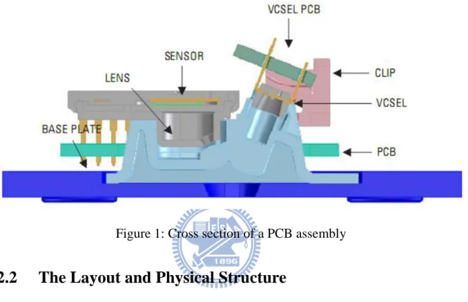
2.1.3 Optical Sensor
The optical sensor used in this prototype is from Avago Technologies and its reference number is ADNB-6012-EV. This sensor is based on a laser diode, which allows operating on many surfaces that prove difficult for traditional LED-based optical navigation. It also has high-performance architecture, which is capable of sensing high-speed mouse motion – with resolution up to 2000 counts per inch.
The subcomponents of this optical sensor include: an optoelectronic sensor with CMOS technology; a lens base, which is used to attach the optoelectronic;
laser diode (VCEL), which also is attach to the lens base; a clip to attach properly the laser diode to the lens base;
a base plate, which is attached to the PCB of the whole prototype. On Figure 1 all parts of the optical sensor are illustrated.
Figure 1: Cross section of a PCB assembly
2.2
The Layout and Physical Structure
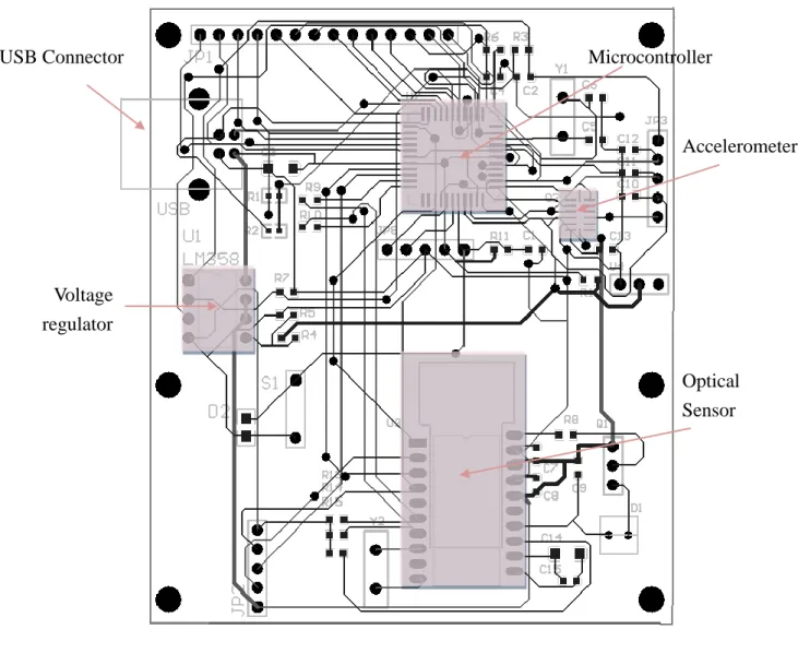
The schematic and layout of the prototype were designed by using the software Protel 99. This program allows creating the schematic circuit including all components described in the previous sections and other elements, such as capacitors, resistors and voltage regulators. Once designed the schematic, the software also can generate automatically a PCB board including all circuit units and route the connection between them. The final PCB layout from the prototype is illustrated in Figure 2.
After the PCB is manufactured, all elements in the circuit are welded in the PCB board. Since the idea of this prototype is to behave as a mouse device, a physical structure of a commercial mouse was used to cover the PCB board. Also, a flat base plate was designed to be attached under the circuit board. In the base plate, there is an orifice, where the laser diode can reach the surface that it operates.
Figure 2: Prototype's layout
2.3
Software Development
2.3.1
USB Drivers and Device Classes
Any hardware device that interacts with a computer program must use a device driver, which is responsible to translate data between the operation system running in the computer and in the embedded system. In this project, the prototype represents the hardware device, which is connected to the computer using a USB port. In this way, the computer and the prototype must use a USB bus driver. Nowadays, many computer
USB Connector Accelerometer Optical Sensor Voltage regulator Microcontroller
peripherals use an USB port to connect to a computer, such as printers, USB flash drives, webcams, keyboards and mouse devices. For each case, not only the USB Bus driver is used, but also a device class that specifies the device’s functionality. In this project, two different device class based on USB are used:
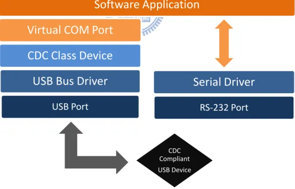
Communications device class (USB CDC), which provides an easy way to read and write any kind of data from/to an USB device. In this thesis, this device class is used to emulate a COM port, which will allow a software application running in the computer to manipulate an USB device as a RS-232 device. Therefore, a simple application can be implemented to read data from the prototype, specifically the sensors data processed by the microcontroller. A comparison between how the kernel and operating system treat a virtual COM port and a regular COM port is illustrated in Figure 3.
Figure 3: Hierarchy from Software Application to USB device
Human Interface device class (USB HID), which stands for human interface
Software Application
Virtual COM Port
CDC Class Device
USB Bus Driver
USB Port
Serial Driver
RS-232 Port
CDC Compliant USB Devicedevices, such as keyboards, game controllers and mouse devices. In this thesis, this device class is used to treat the prototype as a typical mouse device, which means the data sent from the prototype to the computer will be used to move the cursor on the screen. The packet format required when using the HID device class for a regular mouse device consists in 4 bytes:
First byte: it is used to specify the state buttons of the mouse, (1 = pressed, 0 = not pressed), which allows processing simultaneously 8 different buttons. In the prototype, no buttons were added, since only the movement in X and Y directions are analyzed.
Second byte: it is used to specify the displacement in the X coordinate. This is an 8 bit signed variable, which can assume values from -128 to 127. The value ZERO means that no displacement was detected.
Third byte: it is used to specify the displacement in the Y coordinate. The same description from the X coordinate is applied here.
Forth byte: it is used to specify the displacement from the mouse wheel. It is also an 8 bit signed variable, where the signal corresponds which direction the wheel was rolled.
2.3.2
Host Application
A host application was created to read the data from the prototype and process it for generating graphics based on different velocity estimators. This application is written in Matlab script, which can easily be used to plot large amount of data. For this case, the USB CDC device class is used. Therefore, the Matlab script application can connect to the prototype as a serial device, by using functions to open, read and write a serial port.
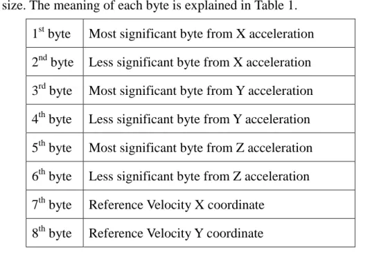
In this scenario, the prototype will be responsible to send binary packets with 8 bytes of size. The meaning of each byte is explained in Table 1.
1st byte Most significant byte from X acceleration 2nd byte Less significant byte from X acceleration 3rd byte Most significant byte from Y acceleration 4th byte Less significant byte from Y acceleration 5th byte Most significant byte from Z acceleration 6th byte Less significant byte from Z acceleration 7th byte Reference Velocity X coordinate
8th byte Reference Velocity Y coordinate
Table 1: Binary packet sent by the prototype
The last two bytes can refer to the optical sensor data or the velocity estimated by one of the integrator techniques implemented in the microcontroller. However, the integrator technique will be only implemented in the microcontroller after choosing the best option among the techniques implemented in Matlab, which has the following flow chart:
Colecting Data
• Open a COM port
• Write a command in the COM port to trigger the prototype • Start reading each 8 bytes, parsing it and storing in vectors
Estimate the velocity
• Based on the the acceleration data collected, the velocity is estimated by using different techniques to integrate the acceleration
• For each estimator technique, a vector of containing the velocity is created • The velocity curve from the optical sensor is built
Plotting the Results
• The raw acceleration of X, Y and Z are plotted.
• The optical sensor velocity curve and the estimator technique velocity curves are plotted in the same graphic for X and Y axes.
Based on the plotted velocity curves, it is possible to define which techniques present the best performance. Once the best techniques are defined, their algorithms will be implemented in the microcontroller embedded in the prototype. The same USB CDC driver and the same software application running in the computer can be used to validate the porting of this algorithm to the microcontroller. The embedded application only has to substitute the optical sensor measurements for the velocity estimated by the technique ported in the microcontroller. When plotting the graphic results using the host application, the curves from the ported estimate technique and the original implementation in Matlab must be similar. They will not be totally the same because the microcontroller has a limited architecture; implicating some parts of the algorithm are implemented with fix point representation. In Matlab, all variables are represented as floating numbers.
The script is structured in different files. Each file will be clarified on next:
“runapp.m”, it is responsible to open the COM port and collect the data from the prototype;
“plotall.m”, it will plot all graphics for data analysis;
“kalman_filter.m”, this is a function file, which is responsible for estimating the velocity by using the Kalman filter. The output is a velocity vector and the input is the acceleration signal of one axis.
“fuzzy_integrator.m”, this is a function file, which uses a fuzzy-neural network to estimate the velocity. The output is also a velocity vector and the input is the acceleration signal of one axis.
“state_machine.m”, a function file that uses a series of different states to estimate the velocity. It has the same inputs and outputs from the other cases. “kalman_state.m”, it is a combination between Kalman filter and state
“combined_sm.m”, a function file that combine the state machines from axes X and Y, where the inputs are the acceleration signal of both axes and the output is the a velocity matrix containing the velocities in X and Y.
2.3.3
Embedded Application
The embedded application is written in C language and the compiler used is CCS C Compiler, which supports Microchip PIC 18x series. One of the advantages of using this compiler is its support to different USB device classes, including HID USB and CDC USB device classes. Therefore, a simple API is provided to access the USB driver. The applications running in the prototype can be developed and compiled in the host machine, and the resultant firmware is downloaded to the target by using a programmer provided by Microchip called MPLAB ICD 2, which uses JTAG protocol to transfer the binary file from the host machine to the microcontroller PIC.
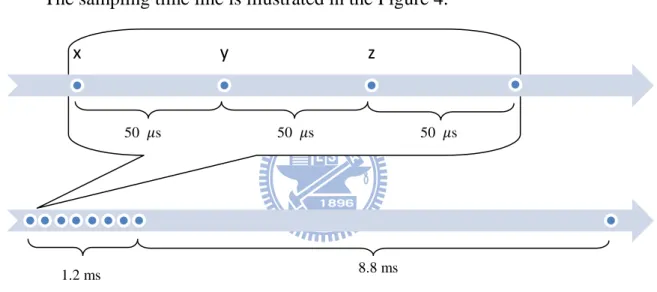
The main program to be executed in the microcontroller consists in a main loop flow that reads the sensor data, process it and send the result to the host machine. The sensor readings are split in two parts. The first part reads the optical sensor using the SPI protocol. The resultant data is two bytes; each byte represents one of the XY coordinates. The second part is responsible to read the accelerometer sensor by using three analog-to-digital converters from the microcontroller. For each axis (XYZ), eight consecutive measures are made and the mean value of them is used to smooth the results. The microcontroller only allows selecting one ADC channel at a time, and for each measurement a delay must be specified to quantize the correct value of the acceleration, which will define the sampling rate of the measurements. This delay is defined in agreement with the maximum sampling rate allowed in the ADC from the microcontroller. Besides that, the delay cannot be too short, or the accuracy of the result will be distorted. Also, it cannot be too long, or the final number of packets per
second send to the host machine will be too small. For instance, the number of packets per second that a commercial mouse device sends to the computer is around 100 packets per second, where each packet corresponds to the format commented in section 2.3.1. Therefore, considering the time to measure all axes is 15% of the time between two consecutive packets, the sampling time of the accelerometers should be smaller than 1.5 ms, which will let around 8.5 ms for the embedded application process the data and integrate the acceleration. In this way, the quantize time for each ADC measurement is defined to 50 s.
The sampling time line is illustrated in the Figure 4.
Figure 4: Sampling time line
Note that the time to process the data and integrate the acceleration is not necessary 8.8 ms; that graphic is only an estimation of the minimum sample rate necessary to similarly perform as the commercial mouse devices.
The flow chart of the main program will be explained in details on next. Some parts of the flow will be explained in the next chapter.
x y z
50 s 50 s 50 s
Chapter 3. Signal Processing Methods
3.1
Data Preparation
Before using any technique to integrate the acceleration signal coming from the three-axis accelerometer, it is necessary to prepare the data by applying some statistical techniques, filters and calibration.
3.1.1 Statistical Techniques
The first step, already commented in the section 2.3.3, is to obtain the average of N acceleration values collected in a high speed sample rate. The following equations are used to obtain a more accurate acceleration:
In this project, the number of data N collected each time is equal 8. Another formula applied in the signal collected in high speed sample rate is the amplitude filter, which returns the difference between the maximum and minimum values. This filter is applied exclusively for the Z axis:
The value of can be used as an indicator of the prototype’ state, since the Z axis can measure the vibration of the environment. Usually this vibration is a high frequency noisy signal. However, when the prototype is moving, this vibration tends to increase, which means the amplitude will be higher. This effect can be observed in the Figure 6. The highlighted areas indicate when the prototype is moving.
Figure 6: Raw acceleration from Z Axis (no scale)
3.1.2 Bias filtering
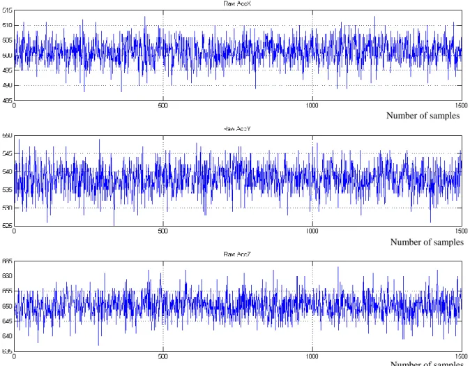
All axes from the accelerometer have an output signal bias which can be observed when no acceleration is applied in that axis. However, if the acceleration of gravity is considered, it can influence in the bias factor of all axis. Since the resolution of the ADC is 10 bits, the acceleration can assume values from 0 to 1024. Ideally, if the accelerometer is not under influence from any force, the acceleration should be around the median value of that scale (512 without scale). However, since the Z axis is in the same direction of the gravity force, its bias will be higher than the other axes, as you see in Figure 7. The average acceleration in X axis of that group of data is 501.34; in Y axis is 537.99; and in Z axis is 650.12.
An inertial mouse device working in a flat surface only requires the integration of X and Y accelerations. Therefore, it is necessary to apply some kind of biased filter to remove the bias factor in both X and Y acceleration signals. A simple way to compensate the signal is to subtract the raw acceleration by the average value
measured when the prototype is stationary. However, this solution may not work well in case the bias factor changes dynamically, which is a common behavior when moving the device in a not totally flat surface.
Figure 7: Raw acceleration of XYZ axes without moving the prototype
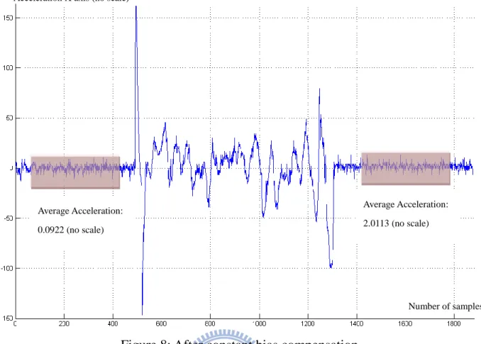
An experimental example of the problem when applying a constant value to compensate the bias factor is illustrated in Figure 8. In that scenario, moving the prototype in one direction just few centimeters was enough to dynamically change the bias factor. The explanation of this variance is related to the tilt angle, which is the angle between the Z axis of the accelerometer and the force of gravity. If the tilt angle is equal zero, the gravity force will not influence the X and Y bias factor. However, if the tilt angle is different than zero, the gravity force will influence the X and Y bias factor proportionally to the tilt angle.
Number of samples
Number of samples
Figure 8: After constant bias compensation
The proposed solution to contour this problem consists in using an Impulse Infinite Response Filter (IIR Filter), which will eliminate the low frequencies and make the acceleration signal to converge slowly to zero. The transfer function in Z domain can be represented as:
Considering the raw acceleration as the input, the final output after applying the filter is the unbiased acceleration . In the discrete time domain, the relation between the input and output can be represented as:
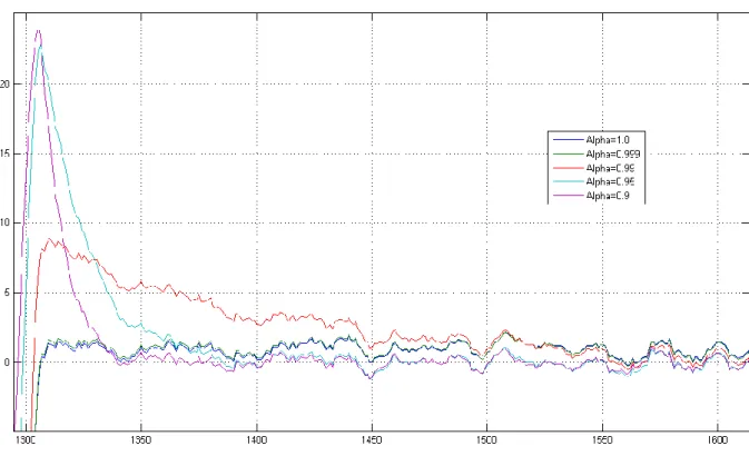
In this formula, the coefficient determines how fast the unbiased acceleration converges to zero. If the coefficient is smaller and close to 1, the influence of the filter is reduced. The behavior of different in the filter can be observed in the Figure 9 . The same data from Figure 8 is used in this analysis.
Average Acceleration: 0.0922 (no scale)
Average Acceleration: 2.0113 (no scale)
Number of samples Acceleration X axis (no scale)
Figure 9: Unbiased acceleration after applying filter H(z) with different : a) , b) , c)
(a)
(b)
Comparing the different scenarios when changing , it is noticed that the case (a) from Figure 9, the distortion is smaller than the other scenarios during the movement. However, in the end of the movement, a small overshoot is observed and the signal converges slowly to zero when comparing with smaller A closer look of the acceleration right before the end of the movement can be observed in the Figure 10.
Figure 10: Closer look in the end of the movement
An optimal solution would be to have an adaptive , that increases when some movement is detected and decreases when there is no movement. In this way, the signal will not be distorted too much during the movement, and in case there is any overshoot in the end of the movement, the filter will converge the acceleration to zero really fast, since will decrease after the displacement. Any movement from the prototype can be easily detected when calculating the average deviation of the signal (next section presents the mathematical formula). If the average deviation is large, the most probably state of the prototype is in movement, otherwise, would be stationary. An example using an adaptive in the biased filter is show in the Figure 11 . Again, the same data from the previous experiments is used. In this scenario, the changes
between 0.9 and 1.0, depending on current average deviation of the acceleration signal. When calculating the average deviation, only the last 15 points were considered.
Figure 11: Adaptive biased filter
3.1.3 Calibration Process
Another important step before apply any estimator technique is the calibration process. In this procedure, some relevant parameters are extracted from the system, which will be used as reference to better estimate the velocity.
Average Absolute Deviation for each axis
The initial task to perform is to identify the average absolute deviation of the all axis from the accelerometer when the prototype is stationary. The formula of the average deviation can be expressed as:
Average Acceleration: 0.0832 (no scale) Average Acceleration: 0.0712 (no scale)
This formula should be applied with for a huge amount of data for each axis (at least 500 samples). The overlap between the points should be considered. Therefore, the formula can be represented in the discrete domain as:
Calculating the histogram from the resultant data, it is possible to extract the most common value of the average absolute deviation, which will be used as one of the calibration parameters.
Discrimination Windows for each axis
During the calibration process, the biased filter can be used to converge the acceleration signal rapidly to zero by setting a small . Once the acceleration reach some value near to zero, is switched to value close to one. In this scenario, the acceleration will assume values around zero when the mouse is stationary, and the noise of the specific axis can be measured. Calculating the histogram of the acceleration after applying the biased filter (note that the average acceleration will be around ZERO), it is possible to identify the amplitude of the noise.
From the histogram, the acceleration value that corresponds to 10% of the most common acceleration level is obtained.
For example, in the histogram on left, the
most common F re que nc y Acceleration
acceleration value is around 0 unit, counting 150 times. 10% of 150 is 15, which corresponds to the acceleration of approximately 10 units.
This acceleration (10 units) will define the discrimination window of the noise. That means any acceleration between -10 and 10 will discriminate as a noise.
Average Value for Z axis
Since the biased filter is only applied for X and Y, only the average value of Z is calculated. Its calculation is straight-forward, the mean value of at least 500 samples from Z axis is obtained when the prototype is stationary.
3.2
The Fuzzy-Neural Integrator
The first technique used to estimate the velocity from the accelerometer signals is based on the fuzzy-neural network. The reason to use this specific combination of two fields – fuzzy systems and neural networks – is because the synergistic integration of them will bring many benefits from both fields. The neural networks provide connectionist structure and learning abilities to the fuzzy logic systems, and the fuzzy logic systems provide the neural networks with a structural framework with high-level fuzzy IF-THEN rule thinking and reasoning. In the theory, there are many possible ways to integrate fuzzy systems and neural networks. The one used in this thesis is called “Fuzzy Modeling Networks”, which the basic idea is to realize the process of fuzzy reasoning by the structure of a neural network and express the parameters of fuzzy reasoning by the connection weights of a neural network. Therefore, it can automatically identify the fuzzy rules and tune the membership functions by modifying the connection weights of the networks using the back-propagation learning algorithmError! Reference source not found..
The configuration type of the Fuzzy Modeling Network is shown in Figure 12. In this particular network, only three inputs are used. Later, a different version of the
Fuzzy-Neural Network will be introduced, including a different number of inputs and nodes; however all of them share the same configuration that will be explained now.
The Fuzzy Modeling Network can be divided into premise part and consequent part. The premise part consists in two layers. The first layer corresponds to the number of inputs of the system, where each input represents a node. The second layer corresponds to the membership functions of each input, where each node presents a fuzzy variable from the membership functions.
The consequence part also has two layers. The third layer corresponds to the fuzzy rules, where each node is the relation between different membership functions. The fourth layer is the output layer, where a unique node represents the final output. The consequence part can be represented as a fuzzy singleton:
On the following sections, the modeling of the Fuzzy Neural Network is explained, including the mathematical model of parts of the network and the learning strategy.
3.2.1 Membership functions
A membership function is defined as the probability of any value from a physical or statistical quantity, such as acceleration, velocity or average deviation, belongs to a specific fuzzy set. Each membership function can contain one or more fuzzy sets, which are related to a linguistic variable. A fuzzy set is a pair where is a set and . On next, some examples of linguistic variable are shown:
Acceleration:{POSITIVE, ZERO, NEGATIVE} Velocity:{POSITIVE, NEGATIVE}
Based on those linguistic variables, it is possible to define the fuzzy sets that will belong to the membership functions of each physical/statistical quantity.
Acceleration
The fuzzy sets that represent each linguistic variable from the acceleration can be expressed mathematically as:
Consider the following parameters are based on the extraction of the discrimination window ( ) during the calibration process explained in section 3.1.3 . The discrimination window represents the interval as ,
were is the acceleration value.
300~400 units
maximum acceleration
Positive Acceleration Zero Acceleration Negative Acceleration Graphically, the above equations represent the following membership function:
Figure 13: Acceleration Membership Function
Velocity
The fuzzy sets that represent each linguistic variable from the velocity can be expressed mathematically as: (where v is the velocity value)
Positive Velocity Negative Velocity
Graphically, the above equations represent the following membership function:
Figure 14: Velocity Membership function
3.2.2 Fuzzy Rules
The fuzzy rules define the relation between the different membership functions. As already commented, singleton rules are used to elaborate the relationship between them:
Where are the inputs of the fuzzy-neural network. And is the result of a specific fuzzy set of the membership function of each input , with , in case the fuzzy-neural network has only three inputs. Mathematically, the result of the node can be expressed as:
The values of is defined in agreement with the singleton rules. For example, imagine a Fuzzy-Neural Network with 3 inputs – the last three accelerations, defined as . And the output is the difference velocity. Using the membership function for acceleration explained in the previous section, the following sentences can be written:
IF is Positive AND is Positive AND is Positive, THEN IF is Negative AND is Negative AND is Negative, THEN IF is Negative AND is ZERO AND is ZERO , THEN
Note that the attribution of the weights is based on physical behavior of a particle submitted to some acceleration.
3.2.3 Defuzzification
Defuzzification is a mapping from a space of fuzzy control actions defined over an output universe of discourse into a space of non-fuzzy control actions Error! Reference
source not found.. The output signal based on the configuration from Figure 12 can be calculate as:
Where is the node values of each fuzzy rule; is weight of each connection
bewteen the fuzzy rule nodes and the output.
3.2.4 Back Propagation Algorithm
The back-propagation learning algorithm is one of the most useful learning techniques used in neural networks. This learning algorithm is applied to multilayer feed forward networks consisting of processing elements with continuous differentiable activation functions.
To better understand how this technique can be used in this project, the following inputs and outputs are defined:
Inputs Output
Current Acceleration: a[n]
Velocity Difference: Previous Acceleration: a[n-1]
Previous Acceleration: a[n-2] Current Velocity: v[n]
Where the accelerations are the measurements coming from the accelerometers and the current velocity is the integration of the acceleration using the Fuzzy-Neural Network.
When using back-propagation algorithm, it is necessary to have the desired output of the system, which will be represented by the optical sensor output. There are 3 phases when using this technique – collecting data, training the network and validation. Each phase will be explained on next.
Collecting Data
In this phase, the training data is created by collecting the last three acceleration signals from accelerometers, the current velocity and the difference velocity from the optical sensor when moving the prototype in one axis. This procedure is performed for X and Y axis. The block diagram of this phase is illustrated in Figure 15.
Figure 15: Block Diagram from Collecting Phase
Once the training data is collected, the Fuzzy-Neural Network is fed with this data. The network’s output is compared to the desired output from the same training data. The error is calculated and propagated back to the network and the weights of each neuron are adjusted. This procedure is illustrated in the Figure 16.
Figure 16: Block Diagram from Training Phase
The equations of the learning algorithm applied in this Fuzzy-Neural Network are explained in the following lines:
The output error measure ( is calculated as:
-
The error is propagated backward to update the weights based on the learning rate :
Splitting in partial differential equations:
The output can be substituted by the equation described in section 3.2.3 and
This is the final equation to adjust the weights of the network part of the Fuzzy-Neural Network.
Validation
In this phase, the output from the trained Fuzzy-Neural Network is compared with the optical sensor signal. If , where is the maximum error acceptable, and . If the average error is below the threshold, no more training is necessary.
Figure 17: Diagram Block from Validation Phase
3.2.5 Fuzzy-Neural Model
The Fuzzy-Neural Network (FNN) proposed in this thesis consists to estimate the velocity of the prototype in one of X and Y axes. Therefore, the FNN has as output how much the current velocity should be incremented or decremented. The inputs of FNN are based on the measured acceleration and the current velocity for a specific axis.
The modeled Fuzzy-Neural Network has the same configuration commented in the section 3.2.4 , when explaining how the back-propagation algorithm works. For
this particular configuration, all layers are quantified by counting the number of nodes, as observed in Table 2. Note that the number of rules is calculated based on number of inputs and the number of fuzzy sets of each input. The general formula is:
Layer 1 Inputs Layer 2 Membership Functions Layer 3 Fuzzy Rules Layer 4 Output
Acceleration a[n] POSITIVE
NEGATIVE ZERO Velocity Difference +
Acceleration a[n-1] POSITIVE
NEGATIVE
ZERO
Acceleration a[n-2] POSITIVE
NEGATIVE
ZERO Current velocity v[n] POSITIVE
NEGATIVE
4 nodes 11 nodes 54 nodes 1 node Table 2: Fuzzy-Neural Network table (first version)
Another thing that is possible to notice is that the fuzzy rules are symmetric. For example, the first rule should have the same absolute value than last rule . That means:
If all input accelerations are positive and the current velocity is positive, the output should be positive with absolute value M.
If all input accelerations are negative and the current velocity is negative, the output should be negative with absolute value M.
The same relation can be done between and , as well as the next symmetric pairs. This specific behavior is used to correct any asymmetry with the weights of the FNN that was calculated using back propagation algorithm, since each weight corresponds to the output of a fuzzy rule. Therefore, consider the trained weighting vector , where is the number of rules. The following equation can be used to correct the asymmetry between the weights.
, where
Another necessary modification on the weighting vector is when the input conditions have all accelerations equal ZERO. In this scenario, the FNN output should be equal ZERO. However, during the integration of the acceleration by using this FNN, it accumulates a lot of errors, which will cause a final velocity different from zero, even if the prototype is stationary. To avoid this behavior, a non-physical assumption is made when establishing the weighting vector:
“If the acceleration is nearly to ZERO, the velocity is also nearly to ZERO” Translating this assumption in a singleton rule, the two following rules should not be influenced when training the FNN:
IF is Zero AND is Zero AND is Zero AND is Positive, THEN
IF is Zero AND is Zero AND is Zero AND is Negative, THEN Where Note that in case that all input accelerations are nearly ZERO, the FNN will “push” the velocity to ZERO as well.
This strategy to train and correct the weighting vector works well if the training data presents large acceleration. However, if the training data includes a significant number of acceleration close to ZERO, which is a common scenario when moving in low velocity, the training can deteriorate the final result of the FNN. For this reason, this algorithm does not work well for movements in low speed. In order to improve the
performance of FNN for low speed, a second version of the FNN is created.
For better performance, the defuzzification process was modified by adding the output of the membership function of the current acceleration to the output signal. The modified Fuzzy-Neural Network is illustrated in the Figure 18. The weight p defines the intensity of the acceleration in the final output.
3.3
The Kalman Filter
The Kalman filter is a set of mathematical equations that provides an efficient computational means to estimate the state of a process, in a way that minimizes the mean of the squared error. The filter is very powerful in several aspects: it supports estimators of past, present, and even future states, and it can do so even when the precise nature of the modeled system is unknown [10].
This filter estimates a process by using a form of feedback control: the filter estimates the process state at some time and then obtains feedback in the form of (noisy) measurements. As such, the equations for the Kalman filter fall into two groups:
time update equations and measurement update equations. The time update equations
are responsible for projecting forward (in time) the current state and error covariance estimates to obtain the a priori estimates for the next time step. The measurement update equations are responsible for the feedback.
The time update equations can also be thought of as predictor equations, while the measurement update equations can be thought of as corrector equations. Indeed the final estimation algorithm resembles that of a predictor-corrector algorithm for solving numerical problems as shown in Figure 19[10].
Figure 19: The discrete Kalman filter cycle
Time Update
("Predict")
Measurement
Update
("Correct")
The Discrete Kalman filter time update equations are expressed as: (Project the state ahead)
(Project the error covariance ahead) Where:
is the state estimation at time k
is the state transition model which is applied to the previous state is the control-input model which is applied to the control vector
is the estimate error covariance is the process noise covariance matrix
The Discrete Kalman Filter measurement update equations are: (Compute Kalman gain)
(Update estimate with measurement ) (Update the error covariance)
Where:
is the Kalman gain is the observation matrix
is the measurement noise covariance matrix is the vector of measurements
3.3.1 The Process to be estimated
In this project, the Kalman filter is used to estimate the velocity based on the accelerations measurements. The position is not relevant here, once only the velocity must be sent to the host machine. Therefore, the state variables of Kalman filter are acceleration and velocity: , where v[k] is current velocity and a[k] is the current acceleration.
The state transition model to represent the relation between the states can be defined base on the physical equation , therefore:
The matrix B, the control-input model, is ignored for this application, since there is no control signal to be applied in this process. Note that represents the period time between two consecutives measurements.
The vector of measurements includes the measurements from the accelerometer and from a tracking model of the velocity, which behaves as a virtual sensor. This tracking model it is also based in the same assumption made when using Fuzzy Neural Network. If the acceleration is nearly to zero, the velocity is also nearly to zero. Therefore, the following equations describe how the tracking model of the velocity works:
Where is the average deviation of the last N points multiplied by the current acceleration, and is the amplitude vibration in Z axis. The final vector of measurements is defined as: . Since there are two measurements variables to be read, the observation matrix is defined as , where is the acceleration scale to convert the quantize value sampled using ADC to a specific scale that can be configure to behave similarly to the scale using optical sensor.
3.3.2 Filter Parameters and Tuning
usually measured prior to operation of the filter. Measuring the measurement error covariance R is generally practical because the process needs to be measured anyway (while operating the filter), so it would be possible to take some off-line sample measurements in order to determine the variance of the measurement noise [10].
The determination of the process noise covariance Q is generally more difficult as typically is not possible to directly observe the process to be estimated. However, the covariance Q matrix can inject uncertainty into the process by selecting the elements from its diagonal. Consider , where is related to the uncertainty of the velocity state and to the acceleration state. When moving in low speed with small acceleration, the signal coming from the accelerometers will be significantly small and the noise will have a large effect in the measurements. For this scenario, should have the same magnitude as . In the other scenario, when moving in high speed with large acceleration, the noise from the accelerometers will not interfere too much in the signal, so should be smaller than .
One way to dynamically change the matrix Q is to fix the value of and apply the following formula for :
However, should be limited in . Note that following points where the acceleration is really small and there is no large deviation, the magnitude of will be as large as , forcing the prediction of the velocity to zero, since the tracking model of the velocity is equal zero to this scenario. In case there is higher acceleration, the tracking model of the velocity will not affect too much the process, since will be smaller than for this scenario.
Using this approach, the matrix covariance Q changes dynamically, which will force the Kalman gain to also change dynamically. Therefore, it will not be
possible to pre-compute this parameter by running the filter off-line.
3.4
The State-Machine Estimator
The Fuzzy Neural Network and Kalman-Filter solutions proposed in this thesis are constantly integrating the acceleration to estimate the velocity. However, this integration may change for different situations, like when moving with high acceleration and low acceleration. A general formula to represent the integration of the acceleration can be expressed as:
The signal coming from the accelerometers has a bias DC component and noise. The bias DC component can be almost totally removed using the bias filter presented in the section 3.1.2 . The noise component can be reduced using the benefits of Kalman Filter and/or Fuzzy-Neural Network. However, the biggest problem that injects uncertainty in the process is the continuous integration, which accumulates error during the movement. This error is proportional to the time of integration ( . Therefore, one way to solve this problem is to break the movement in small parts and ignore the integration of the acceleration after is too large. One way to limit the time of integration is to establish the following rule:
After integrating the first points and the module of velocity assumes a value higher than a specific minimum threshold, the integration of the acceleration should continue until the velocity crosses to zero.
The meaning of this rule is that the user can only move the mouse to one direction. If it tries to change the direction, the acceleration is ignored and the velocity is kept to
zero until the movement is finished. Therefore, the user will not be allowed to change the direction if he does not stop moving the mouse.
Description of State-Machines
State-Machines can be described as a model of behavior composed of a finite number of states, transitions between those states, and actions. For identifying the different behaviors when moving a mouse device, a finite number of states are designed to distinguish the different parts of a movement, especially to determine when the mouse device is not moving,accelerating and decelerating. Different state-machines are proposed to integrate the acceleration. Each one will be explained further in the following sections.
3.4.1 State-Machine using simple integration method
If a state machine is designed to describe the movement of a mouse device, the most obvious and initial state is when the user is not moving the mouse device. This state will be called IDLE state, when the acceleration signal is basically constituted by the intrinsic noise from the accelerometers. When a peak of acceleration is detected, a transition is occurred, changing the state from IDLE to another state called ACCELERATING state. In this state, the acceleration signal is integrated for estimating the velocity. This integration can be really simple, when integrating directly the acceleration signal, or applying some more complex technique, like Kalman Filter. For this initial state-machine, a simple integration of acceleration combined with the trapezoidal method to reduce the error of integration is used. The estimated instantaneous velocity can be obtained by summing the areas between two following sampled accelerometer signals. As observed in the Figure 20.
Figure 20: Approximation of the Instantaneous Velocity
The trapezoid method commented previously consider the area between two sampled acceleration as a trapezoid, instead of a rectangle. The final formula of this area is represented as:
Where is the period between two sampled acceleration signals. Finally, the instantaneous velocity is represented as:
The above equation should be applied when the current state is the ACCELERATING state. A transition will only occur after the acceleration is integrated a minimum number of times and some deceleration is detected. In this scenario, there are two possible states to go. The first one is called HIGH SPEED state, and the second one is LOW SPEED state. The decision is made by observing the current velocity at the moment the transition occurred. If it is higher than a pre-specified threshold, the next state is the HIGH SPEED state, if not, the LOW SPEED state.
velocity is used. However, if the last points of the acceleration are too small, instead of integrating the acceleration, the current velocity is decremented. The reason to apply this strategy is because in case there is any accumulated error of integration after the movement is finished, the velocity will return to ZERO after some cycles.
For the LOW SPEED state, the current velocity also is decremented if the last points of the acceleration are too small. However, for any other situation, the velocity will be kept constant, since when moving the mouse device with low speed, the acceleration signal also is small, which would prejudice the estimation of the velocity.
Once the velocity crosses to zero, a transition occurs, changing from the previous state to STABILIZING state. In this state, the velocity is kept in ZERO until the last points of acceleration are small, which will probably indicate that the user stop moving the device. Once non-movement is detected, the next state will return to IDLE state. The complete state machine is illustrated in Figure 21.
Figure 21: Simple State-Machine
A table with all states, transitions and actions is shown in the Table 3. Note that each axis (X and Y) will use this state machine, therefore the actions are not combined and each state machine may have different current states.
IDLE state
Action
Transitions a: peak detected in the acceleration signal
ACCELERATING state
Action
Transitions
b: deceleration detected and current velocity small c: deceleration detected and current velocity high
LOW VELOCITY state
Action
ELSE
Transitions d: current velocity crosses to zero
HIGH VELOCITY state
Action
ELSE
Transitions e: current velocity crosses to zero
STABILIZING state
Action
Transitions f: average deviation combined with current acceleration is small