使用交疊區塊位移補償之強健適應遞歸解交錯處理

全文

(1)國立交通大學電機學院電子與光電學程碩士論文. 使用交疊區塊位移補償之強健適應遞歸解交錯處理. Robust Adaptive Recursive De-interlacing by Overlapped Block Motion Compensation. 研究生: 王新博指導教授: 張添烜. 中華民國九十六年六月.

(2) 使用交疊區塊位移補償之強健適應遞歸解交錯處理 Robust Adaptive Recursive De-interlacing by Overlapped Block Motion Compensation. 研究生: 王新博指導教授: 張添烜. Student: Sin-Bor Wang Advisor: Tian-Sheuan Chang. 博士. 國立交通大學. 電機學院電子與光電學程碩士論文. A Thesis Submitted to College of Electrical and Computer Engineering National Chiao Tung University in partial Fulfillment of the Requirements for the Degree of Master of Science in Electronics and Electro-Optical Engineering June 2007 Hsinchu, Taiwan, Republic of China. 中華民國. 九十六年. 六月.

(3) 誌. 謝. 首先，要感謝我的指導教授—張添烜博士，在這兩年論文的研究上,給我很多寶貴的意見，也鼓勵我發揮自己的想法和創意，讓我的論文研究能有所突破，並且順利的完成。在職研究上常有時間配合的問題，張教授總是能給予我很大的彈性,讓我能夠兼顧學業和工作。張教授這兩年來的指導，讓我獲得了更多不同於自己工作內容的知識，同時也擴展多方面的視野，並且學習到當面對一個新的研究主題時，如何搜集資料、分析資料，進而完成此主題的研究。從張教授身上所學習的研習技巧，對我日後的工作助益頗深，感激之情，難以言表。. 也要謝謝我的口試委員們，交大電子王聖智教授和清華大學陳永昌教授，感謝你們百忙中抽空來指導我，因為你們寶貴的意見讓我的論文更加完備。. 同時，要感謝公司的同事和一起修課的同學，在課業遇到問題時，總是能給予我很多的意見，幫助我順利的完成交大的學業。. 最後要感謝默默支持我的家人們，我的爸媽、老婆，你們的關懷是我努力最大的支柱。.

(4) 使用交疊區塊位移補償之強健視訊解交錯處理. 研究生: 王新博. 國立交通大學. 指導教授: 張添烜博士. 電機學院摘. 電子與光電學程碩士班要. 電視已經由交錯掃描的裝置(例如 CRT)逐漸轉變為循序掃描的裝置(例如 LCD TV, Plasma TV)，所以解交錯處理(de-interlacing)對於改善整體的視訊品質就變得越來越重要。位移補償解交錯處理(motion compensated de-interlacing)比其他的方法可以提供更佳的視訊品質，但是伴隨著而來極龐大的運算量。這篇論文提出一個方法來對付上述的問題。輸入影像區塊首先用強健位移偵測器(robust motion detector) 來偵測是否為移動區塊 (motion block) 。位移偵測器 (motion detector)使用經過雜訊消除的畫面差異值(field difference)來精緻的描繪出移動物體(motion object)的外形而且從而提供強健位移偵測(robust motion detection)。如果移動區塊(motion block)進一步被偵測為大區域複雜移動畫面的一部份，且因為人眼對複雜的移動影像沒有辦法清楚辨識，則將會用簡易的邊緣方向性解交錯處理(edge-directional de-interlacing)來處理這個區塊。其他的移動區塊(motion block) 則使用交疊式方塊位移補償(overlapped block motion compensation)來處理去降低估測錯誤(prediction error)。為了進一步降低估測錯誤和傳遞錯誤，採用適應性遞歸式位移補償(adaptive recursive motion compensation)去利用前一個解交錯輸出畫面緩衝存儲器(Previously De-interlaced Frame Buffer)儲存全靜態影像(the full still image)來做為最佳的參考畫面(reference frame)。從最後的實驗結果得知我們提出的方法比以前低複雜性的作品高出 2dB。.

(5) Robust Adaptive Recursive De-interlacing by Overlapped Block Motion Compensation. Student: Sin-Bor Wang. Advisor: Dr. Tian-Sheuan Chang. Degree Program of Electrical and Computer Engineering National Chiao Tung University. ABSTRACT With the TV changes from interlaced devices (e.g. CRT) to progressive ones (e.g. LCD TV and Plasma TV), de-interlacing becomes more and more important to improve the overall video quality. In which, motion compensated de-interlacing can provide better quality than others but with heavy computational complexity. This thesis proposes a robust adaptive recursive de-interlacing by overlapped block motion compensation to address above issues. The proposed method first use a robust motion detector to detect the input image block as a motion block or not. The motion detector uses the frame difference with noise reduction to finely describe the shape of motion object and thus provides robust motion detection. If the motion block is further detected as part of large-area complex motion image, this block will be processed by simple edge- directional de-interlacing since human eyes are less sensitive to complex motion images. Other motion blocks are processed by overlapped block motion compensation to reduce prediction errors. To further reduce the prediction and propagation errors, the adaptive recursive motion compensated de-interlacing is adopted by using recursive buffer to store the full still images as the best reference frames. The final experiment shows that the proposed method can achieve 2dB higher than previous works with lower complexity..

(6) Contents Chapter 1 Introduction................................................................................................1 1.1 The scene .........................................................................................................1 1.2 Introduction......................................................................................................1 1.3 Organization of the thesis ................................................................................3 Chapter 2 De-interlacing overview.............................................................................4 2.1 Inter-field de-interlacing ..................................................................................4 2.2 Intra-field de-interlacing ..................................................................................5 2.3 Motion adaptive de-interlacing ........................................................................7 2.4 Motion compensated de-interlacing.................................................................9 2.5 Recursive Motion compensated de-interlacing..............................................11 Chapter 3 Proposed robust adaptive recursive de-interlacing ..............................12 3.1 4x3 overlapped block size..............................................................................13 3.2 Robust motion detector with noise reduction ................................................18 3.3 Reducing computational complexity by detecting large-area complex motion image....................................................................................................................22 3.4 Proposed adaptive recursive de-interlacing with lower propagation errors...25 Chapter 4 Experiment results and performance analysis......................................29 4.1 Performance measurement method................................................................29 4.2 Test video sequences......................................................................................30 4.3 Analysis of computational complexity...........................................................32 4.4 Objective performance comparison ...............................................................34 4.5 Comparisons of subject view .........................................................................37 Chapter 5 Conclusion ................................................................................................42 5.1 Summary ........................................................................................................42 5.2 Concluding remarks .......................................................................................42 5.3 Future work....................................................................................................42 BIBLIOGRAPHY ......................................................................................................43.

(7) Chapter 1. Introduction. 1.1 The scene In order to reduce transmission video data, traditional television displays adopt interlacing as display scanning format because human eyes are less sensitive to flickering details. Now, with the fast development of semiconductor and information technology, current high-definition digital televisions like LCD TV or Plasma TV adopt the progressive format. If interlaced video is played by progressive displays, de-interlacing becomes necessary to convert interlaced video sequences to progressive video sequences. As shown in Fig. 1, if de-interlacing is not done correctly, some defects such as flicker, aliasing and jag will be produced in the motion area. Thus, de-interlacing becomes more and more important in times of emphasizing high-quality image.. Fig.1 Aliasing are produced in the motion area.. 1.2 Introduction De-interlacing methods can be divided into four categories: the intra-field de-interlacing, the inter-field de-interlacing, the motion adaptive de-interlacing and the motion compensated de-interlacing [1]. Intra-field de-interlacing exploits the correlation between neighboring samples in a field, and the inter-field de-interlacing exploits the correlation between neighboring fields in the time domain. For these two types of de-interlacing, there are two widely used lower-complexity methods, Bob and Weave [2]. Weave, also called “Field insertion”, belongs to the inter-field de-interlacing and it directly combines odd field with even field. Its concept is that static objects are shown at the same position for even and odd fields and thus these objects can be reconstructed perfectly by Weave. 1.

(8) Thus, it is not suitable for moving objects or the aliasing will be produced. Bob belongs to the intra-field de-interlacing and it uses a single field to reconstruct one progressive frame. Because the vertical resolution of de-interlaced frame is a half of original frame, aliasing or blur will often occur in the output frame. To eliminate aliasing, some edge-directional de-interlacing methods were proposed [3][4]. Doyle et al. [5] proposed edge-dependent interpolation method that uses a larger neighborhood of interpolated pixel to predict edge orientation, and using original pixels of edge orientation to produce interpolated pixels. The motion adaptive de-interlacing uses a motion detector to detect where the motion areas are in whole interlaced field. If detected results are static areas, Weave is used to process these areas. The lost image data in these areas can be recovered perfectly. If detected results are motion areas, the intra-field de-interlacing is used to process these areas. Intra-field de-interlacing can be Bob or edge-directional interpolation etc. The motion adaptive de-interlacing is a practical method which can improve the de-interlaced video quality if the motion detector is very accurate. Otherwise, aliasing or blur will occur in the de-interlaced frame output. To further improve the image quality in motion areas, many motion compensated (MC) de-interlacing methods [6][7][8] were proposed. Motion compensated de-interlacing methods can be divided into two categories: the motion compensated de-interlacing and the recursive motion compensated de-interlacing [11][12]. MC de-interlacing means that reference data are original fields when doing motion estimation [1]. In contrast, recursive MC de-interlacing means that reference data are de-interlaced frames. Schutten and Haan proposed an object-base true motion estimation algorithm [13] which compensates interlaced frames to progressive ones according to true-motion of objects. Wang et al. proposed time-recursive de-interlacing [14], and de-interlaced frame output consists of original pixels of current field and interpolated pixels of previously de-interlaced frame. Motion compensation can improve the quality of images in motion areas, but motion estimation needs higher computation effort. In summary, current de-interlacing methods suffers from detective errors of motion detection [15], predictive errors of motion estimation [1], propagation errors of recursive MC de-interlacing [1] and higher computational complexity [15]. In this thesis, we propose an adaptive recursive motion compensated de-interlacing with 4x3 overlapped block size to address above issues.. 2.

(9) 1.3 Organization of the thesis The rest of the thesis is organized as following. The prior de-interlacing methods are briefly described in chapter 2. The proposed methods are illustrated in chapter 3. The experimental results and comparisons with the prior de-interlacing methods are shown in chapter 4. Chapter 5 is the conclusion of this thesis.. 3.

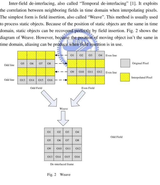
(10) Chapter 2. De-interlacing overview. According to different architectures, we can distinguish four categories of de-interlacing algorithms: the inter-field de-interlacing, the intra-field de-interlacing, the motion adaptive de-interlacing and the motion compensated (MC) de-interlacing. Moreover, the motion compensated de-interlacing can be divided into two categories: the motion compensated de-interlacing (non-recursive) and the recursive motion compensated de-interlacing. We illustrate these de-interlacing methods in order.. 2.1 Inter-field de-interlacing Inter-field de-interlacing, also called “Temporal de-interlacing” [1]. It exploits the correlation between neighboring fields in time domain when interpolating pixels. The simplest form is field insertion, also called “Weave”. This method is usually used to process static objects. Because of the position of static objects are the same in time domain, static objects can be recovered perfectly by field insertion. Fig. 2 shows the diagram of Weave. However, because the position of moving object isn’t the same in time domain, aliasing can be produce when field insertion is in use. O1 Odd line. O5. O6. O7. O13. O14. O15. O3. O4. Even line Original Pixel. O8 O9. Odd line. O2. O10. O11. O12. Even line Interpolated Pixel. O16. Odd Field. Even Field. Weave. O1. O2. O3. O4. O5. O6. O7. O8. O9. O10. O11. O12. O13. O14. O15. O16. Odd Field. De-interlaced frame. Fig. 2 Weave. 4.

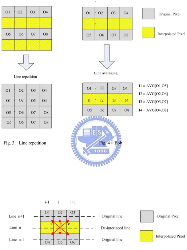
(11) 2.2 Intra-field de-interlacing Intra-field de-interlacing, also called “Spatial de-interlacing” [1]. It exploits the correlation between neighboring pixels in a field when interpolating pixels. The simplest form is line repetition. Fig. 3 shows the diagram of line repetition. This method produces interpolated pixels from vertically upper pixels or down pixels. Additionally, other one of the simplest form is line averaging, also called “Bob”. Fig. 4 shows the diagram of Bob. This method produces interpolated pixels from the average between vertically upper pixels with down pixels. In addition to above methods, the edge-directional de-interlacing is very useful too. Fig. 5 shows the diagram of the edge-directional de-interlacing. It exploits the correlation between three pixels in the previous scan line (line n-1) and the next scan line (line n+1) to determine an obvious edge in the image. The path a is the difference between original pixel 1(O1) and original pixel 6(O6), the path b is the difference between original pixel 2(O2) and original pixel 5(O5), the path c is the difference between original pixel 3(O3) and original pixel 4(O4). Obviously, the path of smallest difference is obvious edge which is used to produce interpolated pixels. Because the architectures of above methods are very simple, these methods have the advantages of low cost and lower computational complexity [15]. However, interpolated pixels consist of neighboring pixels in a field, so interpolated pixel value approximates to real pixel value, is not equal. Therefore, aliasing, jag will appear in de-interlaced video sequences.. 5.

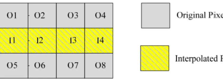
(12) O1. O2. O3. O4. O1. O2. O3. O4. Original Pixel. O5. O6. O7. O8. O5. O6. O7. O8. Interpolated Pixel. Line averaging Line repetition. O1. O2. O3. O4. O1. O2. O3. O4. O5. O6. O7. O8. O5. O6. O7. O8. I1 = AVG[O1,O5]. O1. O2. O3. O4. I1. I2. I3. I4. I3 = AVG[O3,O7]. O5. O6. O7. O8. I4 = AVG[O4,O8]. I2 = AVG[O2,O6]. Fig. 3 Line repetition. Fig. 4 Bob. Fig. 5 Edge-directional de-interlacing. 6.

(13) 2.3 Motion adaptive de-interlacing Up to now, the motion adaptive de-interlacing [17],[18] is a very common method since its architecture is not complex. This method uses a motion detector [1] to detect where the motion areas are in the current field and control the importance or “weight” of these individual pixels at the input of the spatial filter [19]. Therefore, the intra-field de-interlacing is used for motion areas, while the inter-field de-interlacing is used for static areas. Fig. 6 shows the flowchart of the motion adaptive de-interlacing. First, we calculate the difference in corresponding pixels between reference fields and current fields until the last pixel. If the pixel difference is larger than a threshold, the pixel is regarded as the motion pixel. Otherwise, the pixel is regarded as the static pixel. However, this simple method is easily affected by noise. Thus, the outputs of corresponding pixel difference may include some erroneous information and will cause erroneous motion detection. Thus, noise reduction [20] is necessary to eliminate noises in the difference outputs, and provide robust motion detection. General model of noise reduction consists of low-pass filter and rectifier. S-F Lin proposed the morphological operation [15] for noise reduction as shown in Fig. 7. This method uses a 3x3 min filter (low-pass spatial filter) to eliminate noise, and then a 3x3 max filter (high-pass spatial filter) to rectify the shape of motion objects. However, the min filter seriously destroyed the shape of motion objects even though it is rectified with max filter. Therefore, the shape of motion objects can not be recovered any more. To solve this problem, we propose an adaptive noise filter. It eliminates noises in the difference output according to the shape of motion objects. Thus, the shape of motion objects is not destroyed and accurate motion detection is available for later de-interlacing. This method will be illustrated in Section 3.2 in detail.. 7.

(14) Fig. 6 Flowchart of the motion adaptive de-interlacing. F(j-1,k-1). F(j,k-1). F(j+1,k-1). F(j-1,k). F(j,k). F(j+1,k). F(j-1,k+1). F(j,k+1). G(j,k)=MIN[F(j-1,k-1),F(j,k-1),F(j+1,k-1), F(j-1,k),F(j,k),F(j+1,k), F(j-1,k+1),F(j,k+1),F(j+1,k+1)]. D(j,k)=MAX[G(j-1,k-1),G(j,k-1),G(j+1,k-1), G(j-1,k),G(j,k),G(j+1,k), G(j-1,k+1),G(j,k+1),G(j+1,k+1)]. F(j+1,k+1). Fig. 7. the morphological operation. 8.

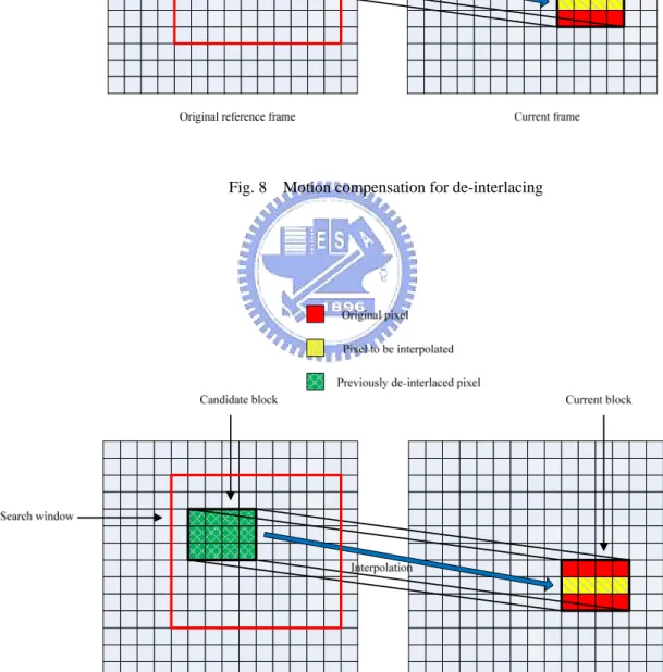
(15) 2.4 Motion compensated de-interlacing Motion compensation is a block-based dynamic compensation technology [16][21]. It uses motion estimation to search the most similar candidate blocks in the neighboring fields, and calculates the offset of corresponding position, as called motion vector (MV) [16]. In the de-interlacing application, they are searched in the neighboring fields because moving objects exist on several continuous video sequences. Fig. 8 shows the diagram of motion compensation for de-interlacing. First, it finds out motion objects in current fields by motion detection, and then motion objects are divided to various current blocks. When searching motion objects, the block-based motion estimation is used to search the most similar candidate blocks in the neighboring fields by SAD (Sum of Absolute Difference) value [16] of candidate block. Finally, the most similar candidate block interpolates the de-interlaced output of current block. Since SAD values of all candidate blocks in the search window [6] needs to be calculated, the required computational complexity is very large and becomes a problem in practical use. Besides the huge computational complexity, the motion compensated de-interlacing has the other problem. This problem is that reference field only contains even lines or odd lines, and it results in motion estimation errors or lower probability of finding the most similar candidate block. Motion estimation errors are erroneous motion vectors which are caused by higher SAD threshold value, and higher SAD threshold value causes unsuitable candidate block to interpolate the de-interlaced output of current block. Lower probability of finding the most similar candidate block is caused by lower SAD threshold value, and lower SAD threshold value causes no suitable candidate block to interpolate the de-interlaced output of current block. Therefore, the recursive motion compensated de-interlacing [13] is proposed to solve this problem.. 9.

(16) Fig. 8. Motion compensation for de-interlacing. Fig. 9. Recursive motion compensation for de-interlacing. 10.

(17) 2.5 Recursive Motion compensated de-interlacing The difference between recursive MC de-interlacing [11][21][22] and MC de-interlacing is that, reference fields of recursive MC de-interlacing are de-interlaced fields instead of original fields when doing motion estimation. Once a perfectly de-interlaced field [1][14] is available, motion estimation is more accurate. A perfectly de-interlaced field is the de-interlaced frame output that the full still image is de-interlaced by field insertion. Because the full still image has no any motion objects in the video image, the de-interlaced frame outputs are the same as original video frames. Fig. 8 shows the diagram of recursive motion compensation for de-interlacing. Its whole procedure is similar to the motion compensated de-interlacing and thus it also has large computational complexity. Besides huge computational complexity, the recursive MC de-interlacing has the propagation error due to the recursive operation. The propagation errors contain motion prediction errors and interpolated errors in previously de-interlaced reference field (frame). To reduce the effect of this problem, we propose an adaptive recursive MC de-interlacing with lower propagation errors. It controls the amount of propagation errors according to video signals, and thus congenital defects of recursive MC de-interlacing are eliminated. This method is illustrated in Section 3.4 in detail.. 11.

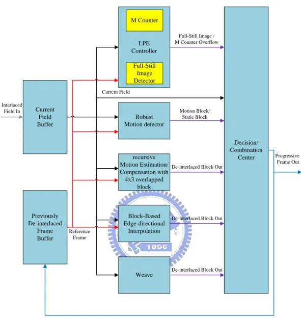
(18) Chapter 3. Proposed robust adaptive recursive de-interlacing. Fig. 10 shows the block diagram of the proposed method. It contains eight major blocks: the current field buffer, the previously de-interlaced frame buffer, LPE (Lower propagation errors) controller, the robust motion detector, the recursive motion estimation/compensation module, the block-base edge directional interpolation module, the Weave module and the decision/combination center. First, the interlaced field data are stored in the current field buffer and the reference frame data are stored in the previously de-interlaced frame buffer. They provide correlative image data for other modules. LPE (Lower propagation errors) controller which contains M counter and Full-still image detector is used to control the amount of propagation errors. Full-still image detector can detect the input interlaced field as a full-still image according to the frame difference. If the frame difference has no any differential value, it outputs the Full-still image signal to the decision/combination center. If the continuous frame differences have differential value, M counter will overflow to reduce the amount of propagation errors by closing the recursive motion compensation. The robust motion detection module is used to provide the robust motion detection, and it indicates that current block is a motion block or a static block. If it is a motion block and the reference block is found, this block will be processed by the recursive motion compensation, but if the reference block is not found or M counter overflow, this block will be processed by the block-based directional edge interpolation. If it is a static block or part of the full-still image, this block will be processed by Weave. The decision/combination center selects the de-interlaced block outputs from the recursive motion estimation/compensation module, the block-base directional edge interpolation module or the Weave module according to these control signals: Full-still image, M counter overflow, Motion Block and Static Block. Finally, it combines the de-interlaced blocks with current fields and outputs the progressive frames. The rest of the chapter illustrates individual modules of the proposed de-interlacing method in details.. 12.

(19) M Counter. LPE Controller. Full-Still Image / M Counter Overflow. Full-Still Image Detector Current Field Interlaced Field In. Current Field Buffer. Robust Motion detector. Motion Block/ Static Block. recursive Motion Estimation/ De-interlaced Block Out Compensation with 4x3 overlapped block. Previously De-interlaced Frame Buffer. Block-Based Edge-directional Interpolation. Reference Frame. Decision/ Combination Center. Progressive Frame Out. De-interlaced Block Out. De-interlaced Block Out. Weave. Fig. 10. Block diagram of the proposed method. 3.1 4x3 overlapped block size The motion compensation is used to improve the de-interlacing quality in video processing. To make sure the de-interlacing quality good, motion estimation must be very accurate. In other words, the more accurate motion estimation can reduce the predictive errors from motion compensation. To get the accurate motion estimation, the overlapped motion compensation is adopted to describe the shape of motion objects in detail.. 13.

(20) Fig. 11 shows the graphical illustration of 4x3 overlapped block size. It uses a 4x3 block to determine the interpolated pixels. However, the block for the consecutive interpolated pixels will be overlapped for accurate motion estimation. As shown in the figure, when interpolated pixels in both the 4x3 A current block and the 4x3 B current block are de-interlaced, they will use the same overlapped pixels in line n. Thus, the 4x3 A current block and the 4x3 B current block are overlapped. In order to avoid incorrect pixels in the reference block as the compensated values for the interpolated pixels in the current block, we compare both vertically upper pixels and down pixels of interpolated pixels in the current block with de-interlaced pixels in the reference block. If they are similar, the pixels in the reference block are the best solution to the interpolated pixels in the current block. The best overlapped block size is a tradeoff between computational complexity and its benefit. The minimum block size is 2x2 which only includes two original pixels to be compared with candidate block in the reference frame. Thus, it is too small to make accuracy motion estimation. But if current block size is bigger, it can result in bad motion compensation. Table 1 shows experimental results in various block size comparison, the 4x3 overlapped block size has higher PSNR than other block size. These test video patterns in table 1 are illustrated in chapter 4.2. The following shows the proposed block matching rule. Fig. 12 shows the 4x3 overlapped block that includes eight original pixels (O1~O8) and 4 interpolated pixels (I1~I4). Fig. 13 shows the 4x3 overlapped block matching rule. The rule is that the block is matched if eight original pixels (O1~O8) of candidate block in the reference frame are very similar to eight original pixels (O1~O8) of current block in the current frame. In other words, the difference in corresponding pixels between candidate block and current block is very small. The overlapped block matching is described in detail as the following. These eight corresponding pixels (O1~O8) are compared in order, and if the difference of some one is large, the block match fail. In contrast, previous works use the sum of absolute difference (SAD) for matching, which introduce higher complexity. However, SAD is not necessary to be calculated in our proposed method because of the 4x3 overlapped block matching. Thus, the 4x3 overlapped block matching has less computational complexity than the SAD matching. Table 2 shows the computational complexity comparison between these two kinds of matched rules. If the block is matched, we will use the four de-interlaced pixels (D9~D12) in the reference block as the compensated values for the interpolated pixels (I1~I4) in the current block, as shown in Fig. 14.. 14.

(21) Fig. 11. The graphical illustration of 4x3 overlapped block size. 15.

(22) Δ = PSNR (other block size) - PSNR (4x3 block size) 4x3. 2x2. 4x4. 8x8. 16x16. Name PSNR. PSNR. (dB). (dB). Flag. 30.12. 27.25. -2.87. 27.67. -2.45. 27.81. -2.31. 28.14. -1.98. Bus. 31.08. 30.22. -0.86. 29.97. -1.11. 29.83. -1.25. 29.10. -1.98. Stefan. 24.59. 23.71. -0.88. 24.49. -0.10. 24.26. -0.33. 24.34. -0.25. Table Tennis 31.09. 29.52. -1.57. 29.74. -1.35. 29.66. -1.43. 28.59. -2.50. Silent. 32.38. -0.44. 32.48. -0.34. 32.60. -0.22. 32.52. -0.30. 32.82. Δ(dB) PSNR(dB). Δ(dB) PSNR(dB). Δ(dB). PSNR(dB). Δ(dB). Table 1 Various block size comparison. Total instruction counts (Computational complexity) = Arithmetic instruction counts + Data instruction counts Δ = [Total instruction counts (4x3 overlapped block matching) - Total instruction counts (SAD matching)] / Total instruction counts (SAD matching) SAD matching. 4x3 overlapped block matching. Name Total Inst. counts. Total Inst. counts. Δ(%). Flag. 2842096. 1643168. -42.2%. Bus. 1513920. 899464. -40.6%. Stefan. 5497050. 3137868. -42.9%. Table Tennis 1478124. 876623. -40.7%. Silent. 1393264. 875160. -37.2%. Average. 2544891. 1486457. -41.6%. Table 2 The computational complexity comparison between these two kinds of matched rules.. Fig. 12. The 4x3 overlapped block. 16.

(23) Initial value: i =1. Difference = Oi(i+MV,n-1) – Oi(i,n). Is Difference small? NO YES. i>8 No, i+1 YES. Block Match & Compensation. Match Fail. Fig. 13 4x3 overlapped block matching. D1. D9 D5. D2. D10 D6. D3. D11 D7. D4. D12 D8. O1. O2. O3. O4. I1. I2. I3. I4. O5. O6. O7. O8. Original Pixel. Interpolated Pixel. 4x3 current block De-interlaced Pixel. 4x3 reference block. Fig. 14. Compensation of motion block. 17.

(24) 3.2 Robust motion detector with noise reduction We can discover in Fig. 15(a) that the simple motion detection by frame difference will be easily affected by noise and thus produces inaccurate motion detection, as shown in Fig. 15(b). The general noise reduction first uses erosion (Low Pass Filter) [15] and then dilation (High Pass Filter) [15] to the frame difference. However, these processes will destroy the outline of motion object and results in erroneous motion detection, as shown in Fig. 15(c). To keep the outline of motion object, we propose a robust motion detector. First, it scans the frame difference line by line, and if motion pixel is detected, the detection process is enabled. The detection process checks the next pixel and records total number of motion pixel until static pixel is detected or the end of scanning line is reached and these continuous motion pixels will form a current line, as shown in Fig. 16. To reduce the noise effect, we use the following two conditions to check this current line as part of the motion area or not. If it is part of the motion area, we will call it as the motion line. 1. Fig. 17 shows the graphical illustration of condition1. The threshold value is set as two and the current line length must be larger than it. 2. Fig. 18 shows the graphical illustration of condition2. Its neighboring line is a motion line. (either upper or lower neighbor) If condition 1 is satisfied, this current line has enough horizontal width, and if condition 2 is satisfied, this current line has enough vertical width. If both two conditions are not satisfied, this current line may be noise or tiny motion object. Fig. 15(d) shows the result of the proposed method, which can keep the outline of motion object accurately. Therefore, the proposed method describes the shape of motion objects clearly, and motion detection is more precise.. 18.

(25) (a). (b). (c). (d) Fig.15 (a) The original field (b) The original field difference (c) The field difference after erosion and dilation (d) The field difference after proposed noise reduction. 19.

(26) Set of motion pixels. Single mtion pixel. Current line. Fig. 16. Current line. Set of motion pixels. Single mtion pixel. Current line length > threshold. Fig. 17. The graphical illustration of condition 1. 20.

(27) Motion Line Line n+1 Line n Current Line Line length > threshold Case1: current line of line n neighbors with motion line of line n+1 Motion Line Line n+1 Line n Current Line Line length > threshold Case2: current line of line n neighbors with motion line of line n+1 Motion Line Line n+1 Line n Current Line Line length > threshold Case3: current line of line n neighbors with motion line of line n+1 Line length > threshold Current Line Line n Line n-1 Motion Line Case4: current line of line n neighbors with motion line of line n-1. Line length > threshold Current Line Line n Line n-1 Motion Line Case5: current line of line n neighbors with motion line of line n-1 Line length > threshold Current Line Line n Line n-1 Motion Line Case6: current line of line n neighbors with motion line of line n-1. Fig.18. The graphical illustration of condition 2. 21.

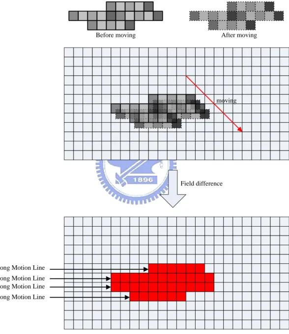
(28) 3.3 Reducing computational complexity by detecting large-area complex motion image Motion compensated de-interlacing has higher computational complexity than spatial (or Intra-field) interpolation due to the motion estimation. To reduce computational complexity, we propose to apply simple spatial de-interlacing for large-area complex motion image. The reason for this is that human eyes are less sensitive to complex motion image and the spatial de-interlacing is enough to provide suitable image quality. With this, we can reduce the complexity. The key point for such method is the detection for large-area complex motion image, which is described as following. The basic idea is that a motion object consists of some adjacent pixels with the same gray level, and those pixels with different gray level are regarded as different objects. Fig. 19 shows a big motion object, in which the motion area is only visible on the outline of motion object, and the inner of motion object is static area. Thus, the motion line length of large motion object must be short. Fig. 20 shows the complex motion image, in which a complex motion image combines with many small motion objects and thus it is filled with many long motion lines mostly. With above observations, the proposed method works as following. First, the field difference is processed by proposed noise reduction filter, and the produced result indicates the range of motion area. Second, the produced result is analyzed once every two lines until all lines are analyzed. If the analyzed line is filled with long motion line mostly, it is regarded as a large-area complex motion image. With this method, we can efficiently reduce the computational complexity as analyzed at the later Section.. 22.

(29) Before moving. After moving. moving. Field difference. Short Motion Line Short Motion Line Short Motion Line Short Motion Line Short Motion Line Short Motion Line Short Motion Line Short Motion Line. Short Motion Line Short Motion Line Short Motion Line Short Motion Line Short Motion Line Short Motion Line Short Motion Line Short Motion Line. Fig. 19. Big motion object. 23.

(30) Before moving. After moving. moving. Field difference. Long Motion Line Long Motion Line Long Motion Line Long Motion Line. Fig. 20. Complex motion image. 24.

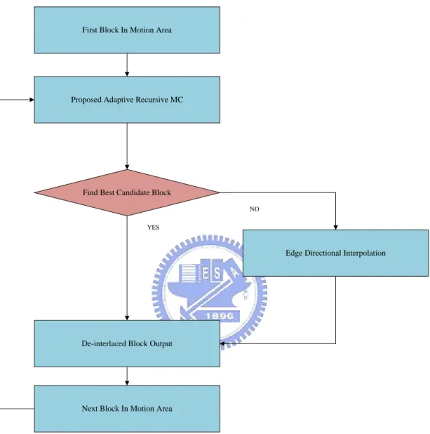
(31) 3.4 Proposed adaptive recursive de-interlacing with lower propagation errors The proposed adaptive recursive motion compensation mainly includes three functions: Motion adaptive de-interlacing with edge directional interpolation, Weave and Edge/MC De-interlacing. Fig. 21 shows the flowchart of Edge/MC De-interlacing. The first block in motion area is processed by the proposed recursive motion compensation to find the best candidate block in the reference frames. If no suitable candidate block is found, Edge directional interpolation is used to process this block, and if the best candidate block is found, this candidate block is the de-interlacing output. Then the next block is processed until all blocks in motion area. For those blocks in static area, they are processed by Weave. Fig. 22 shows the proposed adaptive recursive de-interlacing that has lower propagation errors. The proposed algorithm is described as following. First, the proposed method initializes M counter and the interlaced field data are stored in the current field buffer. The motion detector detects if the current field has motion objects. If the current field has not any motion object, this current field will be processed by Weave. Otherwise, it will be processed by Motion adaptive de-interlacing with edge directional interpolation and the de-interlaced frame output is regarded as the reference frame of next interlaced field. Next interlaced field input the current field buffer, the motion detector detects if this current field has motion objects again. If the current field has not any motion object, the proposed method will set M counter to zero and this current field will be processed by Weave. Otherwise, it will check area of motion objects. If area is very small, this current field will be processed by Edge/MC de-interlacing and M counter will be set to zero since this current field is similar to the full still image. Otherwise, M counter will add up one and be checked if it is overflowing. If M counter is overflowing, this current field will be processed by Motion adaptive de-interlacing with edge directional interpolation since accumulated propagation errors from recursive frame buffer can worsen the de-interlacing quality. If M counter is not overflowing, this current field will be processed by Edge/MC de-interlacing. Finally, this procedure is complete and waiting for next interlaced field input. We use the adaptive motion compensation to control the amount of propagation errors from previously de-interlaced frame. If the current field is the full still image, reference field is merged into current field directly. If several continuous fields have some motion objects and total field numbers exceed the upper threshold of M counter, Edge/MC de-interlacing is disabled and Motion adaptive de-interlacing with edge 25.

(32) directional interpolation is enabled to avoid increasing the amount of propagation errors. In this method, one of key point is the availability of the full still image. For the case that moving speed of motion objects is not too fast, it is very easy that the full still images can be obtained and these images can be the best reference frames for the recursive motion compensated de-interlacing. However, if moving speed of motion objects is too fast, the value of M counter quickly arrives at the upper threshold and no full still image can be obtained. However, in such case, motion adaptive de-interlacing with edge directional interpolation is good enough because human eyes are less sensitive to fast moving objects.. 26.

(33) First Block In Motion Area. Proposed Adaptive Recursive MC. Find Best Candidate Block NO YES. Edge Directional Interpolation. De-interlaced Block Output. Next Block In Motion Area. Fig. 21. Edge/MC de-interlacing. 27.

(34) 1. Initial Process: M=0 2. Interlaced Frame Input. With Motion Objects. Full-Still Image Motion Detection. 1. Motion adaptive de-interlacing with edge directional interpolation 2. De-interlaced frame output as reference frame. 1. Weave 2. De-interlaced frame output as reference frame. Next Interlaced Frame Input. With Motion Objects. Full-Still Image Motion Detection. M=0 No. Is area of motion objects small?. Yes. M=M+1 M=0. 1. Weave 2. De-interlaced frame output as reference frame. No Is M overflow?. Yes. 1. Motion adaptive de-interlacing with edge directional interpolation 2. De-interlaced frame output as reference frame 3. M=0. Fig. 22. 1. Edge/MC De-interlacing 2. De-interlaced frame output as reference frame. Proposed adaptive recursive de-interlacing with lower propagation errors. 28.

(35) Chapter 4. Experiment results and performance analysis. This chapter discusses the experimental results of the proposed de-interlacing method and the performance comparison with other de-interlacing methods. 4.1 Performance measurement method Fig. 23 shows the architecture of performance measurement method. First, the video format of test video sequences is converted from progressive frame (60 Frames/sec) into interlaced field (60 Fields/sec) by interlacing (down sampling). Interlacing (down sampling) is that even lines of original frames are truncated in odd fields or odd lines are truncated in even fields. After de-interlacing, the interlaced fields (60 Fields/sec) are reconstructed into the progressive frames (60 Frames/sec). Then we compare the original progressive video sequences with the de-interlaced video sequences and take PSNR reports.. Test Video Sequences 720x240p 60 Frames/sec. Interlacing (Down Sampling) 720x240i 60 Fields/sec De-interlacing 720x240p 60 Frames/sec Compare. MSE Fig. 23 the architecture of performance measurement method. 29.

(36) 4.2 Test video sequences Fig. 24 shows the test video sequences, including Flag, Bus, Stefan, Table Tennis, Silent, and Rotation. These six test video sequences are different in many aspects. The Flag contains a stationary background with a waved object (flag). The Bus contains a stationary background with some horizontally moving objects (cars). The Stefan contains a complex and moving background with a horizontally moving object (athlete). The Table Tennis contains a complex and stationary background with a vertically moving object (athlete). The Silent contains a stationary background with a vertically moving object (performer). The Rotation contains a monotonously moving background with a rotating object (logo). Therefore, these different kinds of test video sequences provide an objective comparison between various de-interlacing methods.. (a). (b). 30.

(37) (c). (d). (e). (f) Fig.24 Test video sequences (a) “Flag” (b) “Bus” (c) “Stefan” (d) ”Table Tennis” (e) “Silent” (f) “Rotation”. 31.

(38) 4.3 Analysis of computational complexity Δ = [Arithmetic instruction counts (other de-interlacing methods) - Arithmetic instruction counts (Bob)] / Arithmetic instruction counts (Bob) Motion Adaptive directly merge. de-interlacing with 4-Field Adaptive. Bob. Edge-directional. Name. MC[16]. Proposed method. interpolation Arith.. Arith.. Inst.. Inst.. Δ(%). Arith.. Δ(%). Inst. counts counts. Arith.. Δ(%). Inst. counts. Arith.. Δ(%). Inst. counts. counts. Flag. 0. 509760. -. 607680. 19.2%. 3100984. 508.3%. 1109556. 117.7%. Bus. 0. 509760. -. 431112. -15.4% 1229216. 141.1%. 613760. 20.4%. Stefan. 0. 509760. -. 1392288 173.1% 11300976 2116.9%. 2194966. 330.6%. Table Tennis 0. 509760. -. 437664. -14.1% 1280760. 151.2%. 595519. 16.8%. Silent. 0. 509760. -. 415152. -18.6% 1073616. 110.6%. 594460. 16.6%. Rotation. 0. 509760. -. 391920. -23.1% 814840. 59.8%. 646544. 26.8%. Average. 0. 509760. -. 612636. 20.2%. 514.7%. 959134. 88.2%. 3133399. Table 3 Arithmetic instruction counts comparison. Δ = [Data instruction counts (other de-interlacing methods) - Data instruction counts (directly merge)] / Data instruction counts (directly merge) Motion Adaptive directly merge. de-interlacing with 4-Field Adaptive. Bob. Edge-directional. Name. MC[16]. Proposed method. interpolation Data. Data. Inst.. Inst.. Δ(%). Data. Δ(%). Inst. counts counts. Data. Δ(%). Inst. counts. Data. Δ(%). Inst. counts. counts. Flag. 172800 257760 49.2%. 235200. 36.1%. 2111800. 1122.1%. 533612. 208.8%. Bus. 172800 257760 49.2%. 193160. 11.8%. 800080. 363.0%. 285704. 65.3%. Stefan. 172800 257760 49.2%. 422008. 144.2% 7895520. 4469.2%. 942902. 445.7%. Table Tennis 172800 257760 49.2%. 194720. 12.7%. 833320. 382.2%. 281104. 62.7%. Silent. 172800 257760 49.2%. 189360. 9.6%. 687680. 298.0%. 280700. 62.4%. Rotation. 172800 257760 49.2%. 183808. 6.4%. 507960. 194.0%. 330726. 91.4%. Average. 172800 257760 49.2%. 236376. 36.8%. 2139393. 1138.1%. 442458. 156.1%. Table 4 Data instruction counts comparison 32.

(39) Total instruction counts (Computational complexity) = Arithmetic instruction counts + Data instruction counts Δ = [Total instruction counts (other de-interlacing methods) - Total instruction counts (directly merge)] / Total instruction counts (directly merge) Motion Adaptive directly. de-interlacing with 4-Field Adaptive. Bob. merge. Edge-directional. Name. MC[16]. Proposed method. interpolation Total. Total. Inst.. Inst.. Total. Δ(%). Δ(%). Inst. counts counts. Total. Δ(%). Inst. counts. Total. Δ(%). Inst. counts. counts. Flag. 172800 767520 344.2% 842880. 387.8% 5212784. 2916.7%. 1643168. 850.9%. Bus. 172800 767520 344.2% 624272. 261.3% 2029296. 1074.4%. 899464. 420.5%. Stefan. 172800 767520 344.2% 1814296 949.9% 19196496 11009.1% 3137868. 1715.9%. Table Tennis 172800 767520 344.2% 632384. 266.0% 2114080. 1123.4%. 876623. 407.3%. Silent. 172800 767520 344.2% 604512. 249.8% 1761296. 919.3%. 875160. 406.5%. Rotation. 172800 767520 344.2% 575728. 233.2% 1322800. 665.5%. 977270. 465.5%. Average. 172800 767520 344.2% 849012. 391.3% 5272792. 2951.4%. 1401592. 711.1%. Table 5 Total instruction counts comparison. 25000000 directly merge. 20000000. Bob 15000000 Motion Adaptive de-interlacing with Edge-directional interpolation 10000000. 4-Field Adaptive MC Proposed Adaptive Recursive MC with LPE. 5000000. 0 Flag. Bus. Stefan. Fig. 25. Table Tennis. Silent. Rotation Average. Bar chart of total instruction counts. Table 3 shows the arithmetic instruction counts comparison. Table 4 shows the data instruction counts comparison. The data instruction counts include both the load instruction counts and the store instruction counts. Table 5 shows the total instruction 33.

(40) counts comparison. Fig.25 shows the bar chart of total instruction counts. In these results, Bob just needs one arithmetic instruction and two data instructions for every interpolated pixel. Thus its total instructions are fewer than other methods except the directly merge. Motion adaptive de-interlacing with Edge-directional interpolation needs three arithmetic instructions for every interpolated pixel and six data instructions in the motion areas. Thus, its total instructions are middle in all methods. The 4-Field adaptive MC de-interlacing [16] needs to search the most similar motion block in neighboring fields and every candidate block must be checked by calculated SAD value. Thus, total instructions are higher than other de-interlacing methods by several times. In comparison, the proposed method has similar complexity as the simple methods like Motion adaptive de-interlacing and much lower than the 4-Field adaptive MC de-interlacing since our block search method is much simpler and can eliminate operations for large area complex motion blocks.. 4.4 Objective performance comparison Δ = PSNR (other de-interlacing methods) - PSNR (directly merge) Motion Adaptive directly Name. Bob. merge. de-interlacing with 4-Field Adaptive Edge-directional. MC[16]. Proposed method. interpolation PSNR. PSNR. (dB). (dB). Flag. 22.36. 26.94. 4.58. 28.23. 5.87. 27.67. 5.31. 30.12. 7.76. Bus. 26.6. 24.46. -2.14. 30.7. 4.10. 29.97. 3.37. 31.08. 4.48. Stefan. 19.33. 24.09. 4.76. 24.69. 5.36. 24.49. 5.16. 24.59. 5.26. Table Tennis 26.56. 21.42. -5.14. 29.91. 3.35. 29.74. 3.18. 31.09. 4.53. Silent. 30.38. 32.11. 1.73. 32.51. 2.13. 32.48. 2.10. 32.82. 2.44. Rotation. 15.26. 19.5. 4.24. 15.48. 0.22. 15.51. 0.25. 20.2. 4.94. Δ(dB) PSNR(dB). Δ(dB) PSNR(dB). Table 6 PSNR comparison. 34. Δ(dB). PSNR(dB). Δ(dB).

(41) 35 30. directly merge. 25. Bob. 20. Motion Adaptive de-interlacing with Edge-directional interpolation. 15. 4-Field Adaptive MC. 10 Proposed Adaptive Recursive MC with LPE. 5 0 Flag. Bus. Stefan. Table Tennis. Fig. 26. Silent. Rotation. Average. Bar chart of PSNR comparison. Δ = [MSE (other de-interlacing methods) - MSE (directly merge)] / MSE (directly merge) Motion Adaptive directly Name. Bob. merge. de-interlacing with 4-Field Adaptive. Proposed Adaptive. Edge-directional. Recursive MC. MC[16]. interpolation MSE. MSE. Δ(%). MSE. Δ(%). MSE. Δ(%). MSE. Δ(%). Flag. 377. 131. -65.1% 98. -74.1%. 111. -70.5%. 63. -83.2%. Bus. 142. 233. 63.6%. -61.1%. 65. -54.0%. 51. -64.4%. Stefan. 757. 253. -66.5% 220. -70.9%. 231. -69.5%. 227. -70.1%. Table Tennis 143. 468. 226.5% 66. -53.8%. 69. -51.9%. 50. -64.8%. Silent. 60. 40. -32.9% 36. -38.8%. 37. -38.4%. 34. -43.0%. Rotation. 1936. 729. -62.4% 1840. -4.9%. 1828. -5.6%. 620. -68.0%. Average. 569. 309. -45.7% 386. -32.2%. 390. -31.4%. 174. -69.4%. 55. Table 7 MSE comparison. 35.

(42) 10000 directly merge 1000 Bob Motion Adaptive de-interlacing with Edge-directional interpolation. 100. 4-Field Adaptive MC 10. Proposed Adaptive Recursive MC with LPE. 1 Flag. Bus. Stefan. Fig. 27. Table Tennis. Silent. Rotation. Bar chart of MSE comparison. The result of PSNR comparison is shown in Table 6 and Fig. 26, and the result of MSE comparison is shown in Table 7 and Fig. 27. The equations of MSE and PSNR are as followings: FrameSize. MSE (Mean Square Error) =. ∑. ( In – Pn )2 / FrameSize. n =1. PSNR (Peak Signal-to-Noise ratio) = 10 log (2552 / MSE) (unit: dB) Where In denotes the gray value of nth original pixel, Pn denotes the gray value of nth de-interlaced pixel. Peak means the maximum value 255 of 8-bits. In these results, PSNR of the directly merge is much lower than that of other methods. These results are reasonable because motion objects are not shown at the same position in video frames. PSNR of Bob is lower than that of other methods except the directly merge. PSNR of the motion adaptive de-interlacing with Edge-directional interpolation and the 4-Field adaptive MC de-interlacing are similar. In comparison, PSNR of the proposed adaptive recursive MC de-interlacing is the highest, and these results show it has the best quality especially for “Flag” pattern. These results are expectable because our proposed block has high resolution and robust motion detection.. 36.

(43) 4.5 Comparisons of subject view The “Flag” video sequence is used for the comparison of subject view. The original frame, the directly merged frame, the motion adaptive de-interlaced frame, and the proposed adaptive recursive MC de-interlaced frame are shown in Fig. 28(a)-(d), respectively. In directly merged frame, the fluttering flag has seriously jagged phenomenon on the boundary of the flag body. The jagged phenomenon is caused by motion objects which are directly merged with odd fields and even fields, but the background building window has no any influence because it is in the static areas. Compared to the directly merged frame, the motion adaptive de-interlaced frame has an improvement which eliminates most jags, but the question of thickening edge line is still existent. Compared to the motion adaptive de-interlaced frame, the proposed adaptive recursive MC de-interlaced frame has an improvement which eliminates most jags and the thickening edge line since our proposed block has high resolution and robust motion detection. The “Stefan” video sequence is for the comparison of subject view. The original frame, the directly merged frame, the motion adaptive de-interlaced frame, and the proposed adaptive recursive MC de-interlaced frame are shown in Fig. 29(a)-(d), respectively. This video sequence includes a moving athlete and moving background which is caused by the horizontally moving camera, the background includes many audiences and some large-scale words. However, many audiences form a complex image. The audience can’t be clearly distinguished in the directly merged frame, both the moving athlete and the large-scale words have seriously jagged phenomenon on the boundary. Compared to directly merged frame, the motion adaptive de-interlaced frame has an improvement which eliminates most jags. For the complex image of audience, the quality of the motion adaptive de-interlaced frame isn’t so bad because of human eyes are less sensitive to complex image. For the large-scale words, the quality of the motion adaptive de-interlaced frame isn’t so good because of human eyes are sensitive to the large-scale monotonous image. Compared with the motion adaptive de-interlaced frame, the proposed adaptive recursive MC de-interlaced frame has better quality since our proposed block has high resolution and robust motion detection. The “Table Tennis” video sequence is used for the comparison of subject view. The original frame, directly merged frame, the motion adaptive de-interlaced frame, and the proposed adaptive recursive MC de-interlaced frame are shown in Fig. 30(a)-(d), respectively. This video sequence includes upwardly moving ball and arm, 37.

(44) the background is static. In directly merged frame, the arm of athlete has seriously jagged phenomenon on the boundary, and two balls is visible to the eyes. Compared to directly merged frame, the motion adaptive de-interlaced frame has an improvement which ball already can be visible clearly. But the boundary of arm is not still smooth. Compared to the motion adaptive de-interlaced frame, the ball can be visible clearly in the proposed adaptive recursive MC de-interlaced frame, and the boundary of arm is very smooth. Thus the proposed adaptive recursive MC de-interlaced frame shows the best quality since our proposed block has high resolution and robust motion detection.. 38.

(45) (a). (b). (c). (d) Fig.28 Video pattern “Flag”, which frames (a) Original frame (b) Directly merged frame (c) Motion adaptive de-interlacing (d) Proposed recursive motion compensated de-interlacing. 39.

(46) (a). (b). (c). (d) Fig.29 Video pattern “Stefan”, which frames (a) Original frame (b) Directly merged frame (c) Motion adaptive de-interlacing (d) Proposed recursive motion compensated de-interlacing. 40. , reference frame number=1..

(47) (a). (b). (c). (d) Fig.30 Video pattern “Table Tennis”, which frames (a) Original frame (b) Directly merged frame (c) Motion adaptive de-interlacing (d) Proposed recursive motion compensated de-interlacing. 41. , reference frame number=1..

(48) Chapter 5. Conclusion. 5.1 Summary The contribution in this thesis can be mainly summarized into four parts: robust motion detection, accurate motion estimation, lower computational complexity for MC and Algorithm design of the proposed adaptive recursive de-interlacing with lower propagation errors.. 5.2 Concluding remarks In order to improve the performance of de-interlacing, it is difficult for the traditional intra-field de-interlacing. Thus, motion compensation is used to meet this requirement, but it can increase the computational complexity, and if the block size is not suitable for the motion compensation, the predictive errors from motion estimation are produced to worsen the de-interlacing quality. To provide more accurate motion detection/estimation, lower computational complexity, finer images and no jag on the boundary of motion object, four schemes are proposed, including the overlapped block, the proposed noise reduction, the reducing computational complexity by detect large-area complex motion image, and the proposed adaptive recursive motion compensated algorithm. The final experiment shows that the proposed de-interlacing scheme can accomplish lower MSE value, higher PSNR value, and computational complexity is lower than MC de-interlacing methods many times.. 5.3 Future work This thesis proposes the motion compensation de-interlaced method which only adopts the local motion compensation [16], the global motion compensation [16] has not been considered in the proposed de-interlacing. However, the de-interlacing with global motion compensation has better de-interlaced quality for the scaled motion object, but it will bring heavy computational complexity. Thus, it is important work in future that how to provide a global/local motion compensation de-interlacing with lower computational complexity.. 42.

(49) BIBLIOGRAPHY [1]. G. De Haan and E. B. Bellers, “Deinterlacing-an overview”, Proceedings of the IEEE, vol.86, Issue. 9, pp. 1839-1857, Sept. 1998.. [2]. Microsoft Corp., “Broadcast-enabled computer hardware requirements,” in WinHEC’97, Broadcast Technologies White Paper, 1997, pp. 11–12.. [3]. H. Jiang and C. Moloney, “A new direction adaptive scheme for image interpolation,” in IEEE Int. Conf. Image Processing, 2002, pp. 369–372.. [4]. M. Zhao and G. de Haan, “Intra-field de-interlacing with advanced up-scaling methods,” in Proc. ISCE, Reading, U.K., Sep. 2004, pp. 315–319.. [5]. T. Doyle and M. Looymans, “Progressive scan conversion using edge information,” in Signal Processing of HDTV II, L. Chiariglione, Ed. Amsterdam, The Netherlands: Elsevier, 1990, pp. 711–721.. [6]. X. Gao, J. Gu, J. Li “De-interlacing Algorithms Base on Motion Compensation”, IEEE Transactions on Consumer Electronics, vol. 51, No. 2, MAY 2005.. [7]. K. Sugiyama and H. Nakamura, “A method of de-interlacing with motion compensated interpolation,” IEEE Trans. Consum. Electron., vol. 45, no. 3, pp. 611–616, August 1999.. [8]. D. Van de Ville, W. Philips, and I. Lemahieu, “Motion compensated de-interlacing for both real time video and still images,” in Proc. Int. Conf. Image Processing, vol. 2, 2000, pp. 680–683.. [9]. G. De Haan, “Motion compensated de-interlacing, noise reduction, and image rate conversion,” Trans. Consum. Electron., vol. 45, no. 3, pp. 617–624, Aug. 1999.. [10] http://www.mpeg.org/MPEG/index.html [11] G. de Haan and E. B. Bellers, “De-interlacing of video data,” IEEE Trans. Consumer Electron., vol. 43, pp.. 819–825, Aug. 1997. [12] G. de Haan and P. W. A. C. Biezen, “Time-recursive deinterlacing for high-quality television receivers,” in. Proc. Int. Workshop HDTV’95, Taipei, Taiwan, Nov. 1995, pp. 8B25–8B33. [13] R.. J.. Schutten. and. G.. de. Haan,. “Real-time. 2–3. pull-down. elimination. applying. motion. estimation/compensation in a programmable device,” IEEE Trans. Consum. Electron., vol. 44, no. 3, pp. 930–938, Aug. 1998. [14] F. M. Wang, D. Anastassiou, and A. N. Netravali, “Timerecursive deinterlacing for IDTV and pyramid. coding,” Signal Process.: Image Commun. 2, pp. 365–374, 1990. [15] S.-F. Lin, Y.-L. Chang, and L.-G. Chen, “Motion adaptive interpolation with morphological operation and 3:2. pull-downed recovery for de-interlacing,” in IEEE Int. Conf. Multimedia Expo, Lausanne, Switzerland, Aug. 2002, CD-ROM. [16] Y.-L. Chang, S.-F. Lin, C.-Y. Chen, and L.-G. Chen, “Video De-Interlacing by Adaptive 4-Field. Global/Local Motion Compensated Approach” in IEEE Transactions on Circuits and Systems for Video Technology, vol. 15, no. 12, December. 2005.. 43.

(50) [17] M. Achiha, K. Ishikura, and T. Fukinuki, “A motion-adaptive high-definition converter for NTSC color TV. signals,” SMPTE J., vol. 93, no. 5, pp. 470–476, May 1984. [18] A. M. Bock, “Motion-adaptive standards conversion between formats of similar field rates, signal. processing,” Image Commun., vol. 6, no. 3, pp. 275–280, June 1994. [19] P. Haavisto, J. Juhola, and Y. Neuvo, “Scan rate up-conversion using adaptive weighted median filtering,” in. Signal Processing of HDTV II, L. Chiariglione, Ed. Amsterdam, The Netherlands: Elsevier, 1990, pp. 703–710. [20] G. De Haan, “Motion compensated de-interlacing, noise reduction, and image rate conversion,” Trans.. Consum. Electron., vol. 45, no. 3, pp. 617–624, Aug. 1999. [21] G. de Haan and P. W. A. C. Biezen, “Sub-pixel motion estimation with 3-D recursive search block matching,”. Signal Process.: Image Commun., pp. 229–239, 1994. [22] G. de Haan and J. Kettenis, “‘System-on-Silicon’ for high quality display format conversion and video. enhancement,” in Proc. ISCE’02, Sep. 2002, pp. E1–E6. [23] O. Kwon, K. Sohn and C. Lee, “Deinterlacing using Directional Interpolation and Motion Compensation”. IEEE Transactions on Consumer Electronics, vol. 49, no. 1, February. 2003. [24] U.S. Patent 6,606,126 B1. Deinterlacing method for video signals based on motion-compensated. interpolation [25] U.S. Patent 6,577,345 B1. Deinterlacing method and apparatus based on motion-compensated interpolation. and edge-directional interpolation [26] U.S. Patent 2006/0023119 A1. Apparatus and method of motion-compensation adaptive deinterlacing. [27] U.S. Patent 2005/0163219 A1. Method for motion vector de-interlacing. 44.

(51) 作. 者. 簡. 歷. 姓名: 王新博籍貫: 高雄市. 學歷: 國立台灣科技大學電子工程學系. 學士 (民國 79 年 09 月 ~ 民國 83 年 06 月). 國立交通大學電機學院在職專班. 碩士 (民國 94 年 09 月 ~ 民國 96 年 06 月). 經歷: 凌陽科技技術開發工程師. 45.

(52)