Tracking Control of Unicycle-Modeled Mobile
Robots Using a Saturation Feedback Controller
Ti-Chung Lee, Kai-Tai Song, Associate Member, IEEE, Ching-Hung Lee, and Ching-Cheng Teng
Abstract—The tracking control problem with saturation
con-straint for a class of unicycle-modeled mobile robots is formulated and solved using the backstepping technique and the idea from the LaSalle’s invariance principle. A global result is presented in which several constraints on the linear and the angular velocities of the mobile robot from recent literature are dropped. The pro-posed controller can simultaneously solve both the tracking and regulation problems of a unicycle-modeled mobile robot. With the proposed control laws, the robot can globally follow any path spec-ified by a straight line, a circle or a path approaching the origin using a single controller. As demonstrated, the circular and parallel parking control problem are solved using the proposed controller. Computer simulations are presented which confirm the effective-ness of the proposed tracking control law. Practical experimental results validate the simulations.
Index Terms—Mobile robots, motion control, nonlinear systems,
stability, time-varying systems, tracking.
I. INTRODUCTION
C
ONTROL problems involving mobile robots have recently attracted considerable attention in the control community. Mobile robots with a steering wheel (unicycle) or two indepen-dent drive wheels are examples with substantial engineering in-terest. Most wheeled mobile robots can be classified as nonholo-nomic mechanical systems. Controlling such systems is, how-ever, deceptively simple. The challenge presented by these prob-lems comes from the fact that a motion of a wheeled mobile robot in a plane possesses three degrees of freedom (DOF); while it has to be controlled using only two control inputs under the non-holonomic constraint. Several researchers indicated, based on Brockett’s theorem [9], that such a system is open-loop control-lable, but not stabilizable by pure smooth, time-invariant feed-back [4], [34]. That is, there does not exist a smooth or continuous feedback law that can stabilize the system.The methods used in recent years to solve mobile robot control problems can be classified into three categories. The first category is the sensor-based control approach to navigation problems. The emphasis is on interactive motion planning
Manuscript received March 10, 1999; revised December 10, 1999 and November 2, 2000. Recommended by Associate Editor K. Kozlowski. This work was supported by the National Science Council, Taiwan, R.O.C., under Contracts NSC-88-2212-E159-003 and NSC 89-2213-E009-126.
T.-C. Lee is with the Department of Electrical Engineering, Ming Hsin In-stitute of Technology, Hsinchu 300, Taiwan, R.O.C. (e-mail: tc1120@ms19. hinet.net).
K.-T. Song and C.-C. Teng are with the Department of Electrical and Con-trol Engineering, National Chiao Tung University, Hsinchu 300, Taiwan, R.O.C. (e-mail: [email protected]; [email protected]).
C.-H. Lee is with the Department of Electronic Engineering, Lunghwa Institute of Technology, Taoyuan 333, Taiwan, R.O.C. (e-mail: chlee@mail. lhit.edu.tw).
Publisher Item Identifier S 1063-6536(01)01812-7.
in dynamic environments [43], [46]. Because the working environment for mobile robots is unstructured and may change with time, the robot must use its on-board sensors to cope with the dynamic environment. Most reported designs following this approach rely on intelligent control schemes, such as fuzzy logic control [19] and neural-network learning control [2], [37], [45]. Obstacle motion estimation and environment con-figuration prediction using sensory information are important for proper motion planning [11], [12]. However, since a mobile robot responds to its surroundings in a reactive or reflexive way; the executed trajectory may not be globally optimized.
In the second category, the navigation problem is decomposed into a path planning phase and a path execution phase. A colli-sion-free path is generated and executed based on a prior map of the environment. The executed path is planned using cer-tain optimization algorithms based on a minimal time, minimal distance or minimal energy performance index. Methods for avoiding both static and moving obstacles have been reported in the literature [15], [16], [24]–[27], [41]. In these methods, a collision-free path is planned according to the environment map space-time relations. The mobile robot must follow the planned path employing a path-following controller.
The third category follows the motion control approach, in which a desired trajectory must be tracked accurately. Among these, tracking controller designs employing a simplified linear model have been reported [4], [13]. Song and Li [44] developed an LQR controller based on a linearized state-space model. In their presentation, the tracking errors can be eliminated and the mobile robot can follow the specified trajectories. In the linear model approach, however, the controller works only when the linear velocity is not zero. Under such circumstances, it would be difficult to control the mobile robot to track the specified tra-jectory and in the mean time stop with the specified pose. Con-sequently a more generalized approach is desirable. Nonlinear system theory has been employed to solve this problem [1], [7], [10], [17], [20], [38], [40]. Two main research directions em-ploying nonlinear control design can be distinguished. The first, initiated by Bloch et al. [3], [5], used discontinuous feedback, whereas the second research direction used time-varying con-tinuous feedback, which was first investigated by Samson [40]. Pomet [38] then proposed several smooth feedback control laws. However, though these solve the regulation problem, they were found to yield slow asymptotic convergence. In order to obtain faster convergence (e.g., exponential convergence), an alterna-tive approach was initially proposed by M’Closkey and Murray [32] and taken up in several subsequent studies (see, e.g., [33]). Our approach falls into this third category.
Research on the tracking problem for mobile robots has been extensive [8], [14], [17], [18], [20]–[22], [29], [30], [36]. Using 1063–6536/01$10.00 © 2001 IEEE
Barbalat’s lemma or the backstepping method, control schemes have been proposed for mobile robots to globally follow special paths such as circles and straight lines. Similar results were ob-tained by Fliess et al. [17] using time-reparametrization and the motion-planning properties of differentially flat systems. De-spite this apparent advance, there exist several key restrictions on these applications:
1) In some studies on tracking problems [20], [21], [36], [44], only certain special cases (e.g., straight lines or circles) are solved, where the tracked linear velocity or angular velocity must not converge to zero. These restrictions limit the range of applications and, more importantly, make it impossible for a single controller to treat the regu-lation problem and the tracking problem simultaneously. 2) In other cases [5]–[7], [33], [38], [40], tracking problems
with linear and angular velocities approaching zero re-main unsolved.
In practical applications, it is preferable to solve the tracking problem and the regulation problem simultaneously using a single controller; otherwise, switching between two different types of controllers will be necessary. In this study, we simulta-neously solved the tracking problem and the regulation problem of unicycle-modeled mobile robots without any further assump-tions. Moreover, the bounds on the wheel velocities must be attended to avoid the high-gain control signal. The important saturation constraints on control inputs (the linear and angular velocities) were incorporated in our controller design.
Using the backstepping technique, which is often employed in mobile robot stability problems, we will present a global re-sult. With our approach, mobile robots can globally follow any specified path, including straight lines, circles, or trajectories approaching the origin. Furthermore, several important cases, such as parallel parking, can be solved exploiting the proposed method. To the best of the authors’ knowledge, in the time-varying continuous feedback literature, this is a here-to-fore un-solved research area. The possibility of extensions to other non-holonomic systems, such as the tracking control of a knife edge, will also be discussed. Simulation results as well as practical ex-periments will be presented to illustrate the effectiveness of the proposed tracking control law.
The rest of this paper is organized as follows. Section II de-scribes the formulation of the control problem. Our main results, including the control law and the stability analysis are presented in Section III. Section IV illustrates both simulations and experi-mental results using the proposed tracking controller and a labo-ratory mobile robot. An extended discussion of the experimental results is presented in Section V. Section VI is the conclusion.
II. PROBLEMFORMULATION
The unicycle-modeled mobile robots considered in this paper are a class of computer-controlled vehicles whose motion can be described or transformed into the following model of con-strained movement in a plane:
(1)
Fig. 1. A nonholonomic mechanical system: unicycle-modeled mobile robot.
where are the Cartesian coordinates and is the angle between the heading direction and the -axis. Examples of this model include the widely used front-wheel drive automobiles, automated guided vehicles (AGVs) with a drive and steering wheel (a unicycle) and mobile robots with two independent drive wheels, (see Fig. 1) [35]. Moreover, the knife edge system can also be viewed as an extended unicycle system (1) (see Section V for details). The nonholonomic constraint for the model (1) is
(2) It specifies the tangent direction along any feasible path for the robot and briefly show that a mobile robot with two indepen-dent drive wheels can be described using the unicycle model (1). We assumed that the reference point lies at the midpoint of the two drive wheels. Let and denote the velocities of the left wheel and the right wheel, respectively. The linear velocity and angular velocity of the mobile robot can be described as
and , where represents the
distance between two drive wheels. Thus, it is not difficult to see that the mobile robot kinematic equation can be described using the unicycle model (1) (also see the discussion in Section IV). In a plane, the unicycle system possesses three degrees of mo-tion freedom, but must be controlled by only two control inputs under a nonholonomic constraint. When we consider the state vector , it is straightforward to show that the system (1) is controllable in both position and orientation [35]. Unfor-tunately, we confront a system where linearization results in a loss of controllability, although the nonlinear system is control-lable. In particular, many researchers, based on Brockett’s the-orem [9], showed that such a system is open-loop controllable, but not stabilizable using the pure smooth time-invariant feed-back law [4].
A. Tracking Control Problem with Saturation Constraint
Suppose the reference trajectory satisfies
where the desired linear velocity satisfies , and the desired angular velocity satisfies
. The desired velocities are bounded and uniformly continuous, with and representing saturation bounds obtained from practical restrictions on con-trol inputs and , respectively. Note that in the perfect tracking case, i.e., , , , (3) always holds. In this paper, our main purpose is to solve the following tracking problem for (1).
1) Tracking Problem with Saturation Constraint (TPSC): Find saturation control laws for and with
, such that the mobile robot with
the kinematic equation (1) follows a reference trajectory
. That is, ,
, and .
Using the robot local frame (i.e., the moving coordinate system – in Fig. 1), the error coordinates [23] can be defined as
Therefore, the tracking error model is obtained
(4) For convenience, we chose new coordinates and inputs [35] as
Equation (4) can be rewritten as
(5a) (5b) (5c) With the new coordinates , the tracking problem is now transformed into a stability problem. System (5a)–(5c) is referred as the error model of the TPSC. In the remainder of this paper, the coordinates will be used in solving the tracking problem. Note that every coordinate transformation
used above is invertible, and is
equiv-alent to , , and . Thus, by invertability
of coordinate transformation, if converges to zero then the TPSC is solved.
Remark 1: The TPSC covers two important cases.
Case 1 (Regulation Case): If and , then the TPSC is reduced to the regulation (stability) problem studied in [38].
Case 2 (Tracking Case): If , then the TPSC is reduced to the so-called tracking control problem studied in [20].
It is observed that tracking a straight line or a circular path belongs to Case 2, and the reference trajectory can be described by (3) (see [20] for the straight line case and Section IV for cir-cular paths). However, tracking a path approaching the origin, e.g., the parallel parking problem, has remained unsolved
be-cause for some (violating the
condi-tion given in Case 1) and (thus not
satisfying Case 2).
Remark 2: Because the TPSC covers two different cases, it
will not be easy to solve using a single controller. In fact, there are some differences between Cases 1 and 2. For example, con-sider the following linearized model of (5a)–(5c) at the equilib-rium point (0,0,0):
It can be seen that this linearized model is not stabilizable in Case 1, but stabilizable using the linear feedback controller for
the case for all (a slightly stronger
condition than the condition given in Case 2). On the other hand, the key to study the stability in Case 1 is to use a “persistent exci-tation” input to , (i.e., ) based on LaSalle’s invariance principle [38], while the key to study the stability in Case 2 is to use the “persistent excitation” of and
[i.e., ] [20]. Note that the persistence
of excitation condition is often used to guarantee the stability of an adaptive control system. In the stability issue, the
condi-tions and have
the same effect as the persistent excitation discussed in system identification and adaptive control literature. Based on these ob-servations, a possible solution is to find an input such that is “persistent excitation” to solve the TPSC using a single controller in view of (5a)–(5c) and the hint from LaSalle’s invariance principle. This idea provided the initial motivation for this study. We will first solve the TPSC for the unicycle model (1) and then apply it to a mobile robot with two-inde-pendent drive wheels.
III. GLOBALTRACKINGCONTROLLAWS WITHSATURATION CONSTRAINTS
In this section, a global tracking control law with saturation constraints is derived exploiting the backstepping method and conventional stability theory. The stability of the closed-loop system is guaranteed without any further assumptions relating
to and .
First, let us define the saturation function with as
sgn (6)
Then we define a positive-definite function
Notice that (7) is the square of the distance between the current location of the mobile robot and the desired trajectory. Taking the derivative of along the trajectory of (5a)–(5c) yields
(8) Choosing the saturation control law
(9)
where and . Note that
(10) satisfies the saturation constraint of the linear velocity.
Using the saturation control (9), we have
(11) Next, introduce a new variable
(12)
with , and .
The parameter can be chosen as unity if one of the following conditions holds:
In practical applications, one of the conditions (C1)–(C3) must hold, and can usually be chosen as one. For example, condi-tion (C1) is satisfied in the straight line and circular path cases; condition (C2) holds for the case of tracking a path approaching the origin. However, for completeness, it is necessary to con-sider the case in which none of the conditions (C1)–(C3) is sat-isfied. In this case, is chosen as zero. Note that other specifi-cations of the function in (12) are possible (see Remark 3 after Theorem 1 for details).
We observe that as under the condition that . Thus, the stability of can be guaranteed if converge to zero. With (12), system (5a) is trans-formed into
(13) where
It is easy to check that .
Choose the control law with saturation constraint as (14)
with and . Then
(15)
Note that . So, it is possible to
choose a small and b > 0 such that
. Then
satis-fies the saturation constraint of the angular velocity. Define . We then obtain
(16)
This means that (by the Lyapunov stability
theorem [42]).
Now, we are in a position to present the main result.
Theorem 1: Consider a unicycle-modeled mobile robot (1).
The tracking problem with saturation constraint can be solved
using control laws (9) and (14) with , where
either or can be specified according to the previous discussion.
Proof: see the Appendix. Remark 3:
1) The function can be chosen as with
and for all
[see (A13)]. Obviously, the selection of function depends on the properties of (see the proof in the Appendix).
2) By coordinate transformation, we have
. Therefore, the Lyapunov-like function is just the square of the distance between the current position of the mobile robot and the desired trajectory. It
is clear that if then and .
Consequently, the mobile robot moves toward the target. 3) If only and are bounded, the same result still holds. A deeper stability analysis is required and the proof is omitted here (see, however, [28]).
4) (Perfect tracking case) If the initial error is zero (the mo-bile robot is on the tracked trajectory), then it is easy to see that the tracking errors are also equal to zero at any time.
5) If the saturation constraint constants and are in-finity, then this reduces to a system without saturation constraint. However, in practical systems, there exist constraints on the outputs of the servo motors.
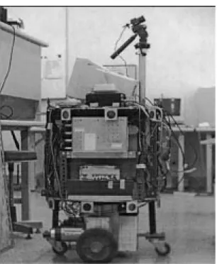
IV. SIMULATIONS ANDEXPERIMENTALRESULTS Fig. 2 shows the experimental mobile robot developed in our laboratory. It has two independent drive wheels and two casters for balance. The kinematic equation can be described using (1)
Fig. 2. The experimental mobile robot developed in the Intelligent System Control Integration (ISCI) Laboratory of National Chiao Tung University.
with and , where
rep-resents the distance between two drive wheels. The proposed controller can be applied to this case with
and . Therefore
(17) In this case, m and the velocities of the left wheel and
the right wheel satisfy the constraint m/s.
Thus, the values of and can be chosen according to the constraint
(18) For and , however, the above inequality is a conserva-tive result. In practical applications, the above condition can be chosen using a simulation procedure. In general, the selection of and would be larger than those determined by con-dition (18).
The proposed control law was first verified using computer simulations. Practical experimental results on the mobile robot then validated the simulated performance. The robot motion is controlled by adjusting the velocities of the left and right wheels. Two HCTL-1100 motion controller chips from Hewlett–Packard were employed for servo control of the two drive wheels. The integral velocity control mode of the chip was used in the experiments to assure satisfactory dynamic response. Fig. 3 depicts the block diagram of the wheel motor control system. The on-board control computer only needs to send commands to the IC chips, which manage the velocity servo control. The position estimation of the robot is conducted using an odometer, which samples the left and right wheel
Fig. 3. Block diagram of the wheel motor control system.
Fig. 4. The developed tracking controller.
velocities to calculate the current posture of the robot. The formula for this estimator is presented in (19)–(23).
(19) (20) (21) (22) (23) where is the sampling period. The architecture of the pro-posed tracking controller is presented in Fig. 4. The models em-ployed in Fig. 4 are described as follows:
Error Model #1: Equation (5a)–(5c); Control law: Equations (9) and (14); Error Model #2:
The desired velocity calculated in the tracking algorithm is transformed into the left and right wheel velocities using
(24) (25) Fig. 5 depicts the implemented tracking control system, which was constructed using the proposed algorithm.
Two trajectories were selected to verify the performance of the proposed control law. In the circular-path trajectory, the tracking performance can be examined. The regulation performance can be further checked with the parallel-parking trajectory. The parameters ( , , , ) are determined by considering the desired tracking performance. In general, large values for and will result in a fast convergence rate
Fig. 5. The implemented tracking control system.
[see the proof of Theorem 1 in the Appendix for the case of ]. In addition, the convergence rate is slightly affected by the parameters and . Experience gained from computer simulations suggested a choice of near 0.5. In the following, tracking as well as docking performance is presented for circular and parallel parking trajectories, respectively. The simulation and experimental results are presented in the same figure for comparison. The models that generate the trajectories are illustrated below
Circular path: (26a) (26b) (26c) (26d) (26e) where ( , ) represents the coordinate of the center and is the radius of the circle. In the simulation and experiment, the
con-stants and are chosen as and m and are
shown in (27a)–(27e) at the bottom of the next page. Fig. 6 il-lustrates the parking place and the designed trajectory. An “8”-shaped trajectory was employed, where 2a and b represent the long and short axis, respectively. In the simulation and
experi-ment, m, m, and . It is easy to check
that the above two trajectories 26(a)–26(c) and 27(a)–27(c) sat-isfy the system (3), with the and given by 26(d)–26(e) and 27(d)–27(e) respectively. Thus, they are perfect tracking cases.
The parameters used in the experiments are presented in Table I. The outputs of the controller were limited as shown in the table, in accordance with the hardware structure of the experimental mobile robot.
For these two cases can be chosen as ,
because the first path satisfies condition (C1) and the second
Fig. 6. The parallel parking place and the designed trajectory.
TABLE I
THEPARAMETERSUSED IN THESIMULATION ANDEXPERIMENTS
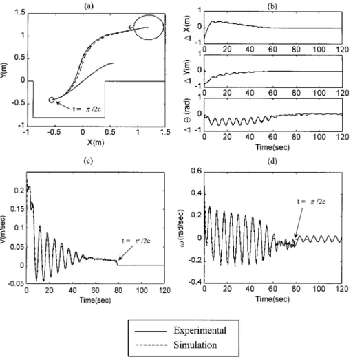
path satisfies condition (C2). Simulation results as well as ex-perimental results with saturation constraints for the circular path and parallel parking are presented in Figs. 7 and 8, respec-tively. In these figures, the dotted lines represent computer simu-lation results and the solid lines represent the corresponding ex-perimental results. In Figs. 7(a) and 8(a), we see that the robot trajectories converge to the desired trajectories. These results demonstrate the capacity of the proposed controllers to produce a nice convergence. The marks in Fig. 7(a) indicate respectively the vehicle and target positions when the target is at the starting point of each lap. In this figure, and , , are the corresponding positions when the target comes to the starting
point at the lap # for the simulation and experiment, respec-tively. We observe that the vehicle tracked the target in the fifth lap. Figs. 7(b) and 8(b) reveal that three tracking errors all con-verge to zero as expected. Figs. 7(c)–(d) and 8(c)–(d) show the recorded controller outputs, namely, the linear velocity and the angular velocity of the vehicle. These outputs are within the limits set in the controller. As shown in Fig. 8, the instant is in-dicated when the vehicle reached the docking point ( , with ). It is observed in Fig. 8(b) and (d) that the experi-mental system shows a slight oscillatory behavior at the docking point. This is caused by the 8-bit resolution of the velocity com-mand used in the experimental system. Note that the oscillation peak of about 0.05 rad/s is practically at the limit of the com-mand resolution. This quantization error in the practical digital control system also resulted in a small orientation error of about 0.05 rad as shown in Fig. 8(b).
It can be seen from Fig. 7 that the experimental results are better than the simulation results. This is due to the mechan-ical damping of the practmechan-ical system and in part by the cyclmechan-ical characteristic of the circular path. As shown in Fig. 7(a), the ex-perimental trajectory did not match the simulation result in the beginning. In fact the mobile robot approached the desired cir-cular path in the inner side with a slower response than that in the simulation, caused by the damping effect. At a later stage, as the target repeated its trajectory in a circle, the tracking controller worked to eliminate the tracking errors and the robot tracked the target. This particular situation resulted in smaller tracking er-rors in the experiment than in the simulation. From Figs. 7 and 8, we observed that the tracking errors all approach zero and the mobile robot follows the desired path. These results confirm the
conclusion in Remark 3 (perfect tracking case). To the authors’ best knowledge, the problems associated with the parking case, with and approaching zero, was previously unsolved in the literature using the nonlinear theory approach. This research effort has proven that the problem can be solved exploiting the proposed controllers (9) and (14). From the proof of Theorem 1, it is observed that the tracking errors converge to zero ex-ponentially if the target keeps moving. However, if the target stops at some point (regulation case) then the tracking errors decay slowly. In this instance, the TPSC is reduced to a regu-lation problem. Therefore, a discontinuous or nonsmooth con-troller is required for fast convergence. For details see [32], [33]. However, the proposed controllers in this paper are smooth con-trollers. It is strongly suggested that proper controller parame-ters should be chosen to produce fast convergence so that the desired path is followed before the target stops.
In this study, for the purpose of comparison, the tracking con-trol problem without any constraint on velocities has also been solved employing a single controller. Fig. 9 presents the exper-imental results of tracking a circular path. It is observed from Fig. 9 that a large control effort and oscillatory transient oc-curred when the mobile robot was controlled by a nonsaturation controller. On the other hand, satisfactory tracking results were obtained using the proposed saturation controller.
This paper only considers the kinematic model of mobile robots. The dynamic model is not included in the main results of this presentation in order to simplify our discussion. It is known that this simplification is acceptable when the system veloci-ties are low, as is in most mobile robot applications. Extending the results for the kinematic model (1) to the dynamic model is
Parallel Parking: (27a) (27b) (27c) (27d) (27e)
Fig. 7. Experimental and simulation results of tracking a circular trajectory. (a) Position variations. (b) Tracking errors. (c) Linear velocity of the center point. (d) Angular velocity.
possible using the backstepping method (see the discussion in Section V). It can be seen from the experimental results shown in Fig. 7(c) and (d) that robot dynamics affect system perfor-mance. Note that the mechanical damping helps to produce a stable, smooth tracking performance. Another factor affecting the experimental performance is the lower-level servo loops. The servo loops have dynamics and the steady-state output of the motors cannot be achieved instantaneously. Normally, this can be managed by proper selection of the sampling time for the tracking controller. In this case, the dynamics and servo sta-bility are assured by implementing the integral velocity control mode of HCTL-1100 motion controller chip.
V. EXTENSION OF THEPROPOSEDMETHOD
The controller design presented in this paper can be gener-alized to other control systems of engineering interest, e.g., the control of a knife edge. We now briefly describe the applica-tion to a knife edge moving in point contact on a plane surface [4]–[7]. With all numerical constants set to unity, the equations of motion are given by
(28)
where and denote the coordinates of the point of contact of the knife edge in the plane and is the heading angle of the knife edge, measured from the -axis; denotes the control force in the direction defined by the heading angle, repre-sents the control torque about the vertical axis through the point of contact and represents the constraint force. The constraint force components arising from the scalar nonholonomic con-straint are described as in (2)
After coordinate transformation, the differential equations can be reduced to an ordinary fifth-order differential equation [4]. Employing the backstepping technique, this control problem can also be solved. We sketch the approach briefly. Let
and . Equation (28) can be trans-formed into
(29a) (29b) (29c) (29d) This is a dynamic system that includes an acceleration term.
con-Fig. 8. Experimental and simulation results of parallel parking. (a) Position variations. (b) Tracking errors. (c) Linear velocity of the center point. (d) Angular velocity.
trollers derived from Theorem 1, where we replace the
satura-tion funcsatura-tion by . Then, is
differ-entiable and the same result as in Theorem 1 holds. Therefore, the knife edge control solution can be designed as and . A similar approach can be applied to study the mobile robot dynamic model with two indepen-dent drive wheels using the backstepping method. The details are omitted due to limited space.
On the other hand, it is also interesting to investigate how to extend the results in this paper to more general driftless systems, e.g., the nonholonomic chained-form systems [35]. However, it seems the approach adopted in this study is not feasible for ap-plication to a general chained-form system with order higher than three. The reasons are stated in the following. First, let us briefly discuss the approach adopted in this paper. Note that the function appearing in (5b) can be approximated by when is small. Thus, a stabilizing virtual controller can
be chosen as such that in
case of and by equation (11). Then, the back-stepping method can be used to guarantee the stability of the whole closed-loop system by choosing a suitable controller such that the virtual error state [defined by (12)] converges to zero, see equation (15). Indeed, a similar argu-ment can be performed for the chained-form systems with order three. This is not the case for chained-form systems having order
higher than three. In fact, it is possible to derive a similar error model like (5a)–(5c) for a general chained-form system with order , however, the nonlinear function will also appear in the error model. The application of the backstepping method in this case will not be straightforward. Thus, it is a challenge to achieve a similar result for chained-form systems or more gen-eral driftless systems.
VI. CONCLUSION
A single controller was developed to simultaneously solve the tracking and regulation problems of a mobile robot. Exper-imental results confirm that the proposed saturation feedback controller gives tracking responses within the physical velocity limitations of the employed mobile robot. It was observed that the executed trajectories were smooth even though the specified trajectory contained nondifferentiable discontinuities. Several directions are interesting for future investigation. The combi-nation of sensor-based navigation algorithms with our proposed tracking controller would give a smooth and precise trajectory in dynamic environments. A recent study on this new area was re-ported by Ma et al. [31] combining a vision system with the nav-igation of a nonholonomic mobile robot. Extending the present result to general chained-form systems remains a challenge for controller design.
Fig. 9. Experimental result: comparison of saturation controller and nonsaturation control for tracking a circular trajectory. (a) Position variations. (b) Tracking errors. (c) Linear velocity of the center point. (d) Angular velocity.
APPENDIX PROOF OFTHEOREM1
A. Several Useful Lemmas
Several technical lemmas, which will be used in the proof of the main results, are described below.
Lemma 1: (Barbalat’s lemma, [42]) If
is uniformly continuous and is finite, then
.
Lemma 2: (Reference [20]) Consider the following system:
where and is bounded and uniformly continuous. If there is a bounded solution solving the above ordinary
differential equation, we have .
Lemma 3: (Reference [39]) Let be a
continuous function. If and
are two bounded functions with , we have
.
For the proofs of Lemmas 1–3, readers may refer to [20], [39], [42]. In the following, two more lemmas relating useful differential inequalities are presented. They will be used in the proof of Theorem 1.
Lemma 4: Suppose , and for all
. Consider the following inequality:
(A1) If , then the following inequalities hold:
1)
2)
Proof of Lemma 4:
1) Let be any positive constant. First claim that
Then, it is clear that
This results in and . Moreover, there is
a positive constant with such that and
for all .
From (A1)
This implies
Thus,
and we reach a contradiction. Therefore, the claim is true for all . This implies that 1) holds.
2) From 1) and , .
Therefore, (A1) can be rewritten as
(A2)
By (A2) and , we obtain
and consequently
This completes the proof.
Lemma 5: Suppose , , and for
all . Assume that is bounded. Consider the
following inequality:
(A3)
If and , .
Proof of Lemma 5: Let us consider the inequality
. Multiplying the term in (A3) by the integral
factor with , we have
and
So, we have
(A4) Thus
(A5) employing the mean-value theorem [39].
Because and is bounded,
and (A5) implies that for all
. Since ,
(see [29]) and hence we have .
This completes the proof.
Before proving Theorem 1, the following lemma is needed.
Lemma 6: Consider the tracking error model (5) with the
control laws defined in (9) and (14). Let be the new variable defined in (12). Then
1) ;
2) There exists a constant such that
and for all and exponentially
decays to zero when ;
3) Trajectories of the closed-loop system are all bounded before the time .
Proof of Lemma 6:
1) It is trivial by (15) and (16).
2) From 1), it is clear that there is a constant
such that and for
all . Then for
all . Note that for all
. Clearly, will exponentially decay to zero.
3) Now, let us prove the boundedness of . Let be
a positive number such that , for all .
Note that (11) gives
(A6) We then have
(A7) Since is positive-definite and radially un-bounded, we conclude that trajectories and
are bounded for all . This completes the
proof.
Now, we are ready to prove Theorem 1.
B. Proof of Theorem 1
is invertible and results in . Thus, studying the stability of the error model (5a)–(5c), is equivalent to studying the stability of the cosystem consisting of (13) and (5b)–(5c). From Lemma 6, we conclude that the trajectories , and are bounded and defined for all . In addition, equation (11) can be rewritten as
(A8) for all by 2) of Lemma 6 and the fact
. From Lemma 6, it is known that con-verges to zero exponentially when . Thus
(A9) By Lemma 4, we conclude that
1)
and 2)
The former tells us that the trajectories of the closed-loop system are also bounded after time . Since is bounded, is uniformly continuous. Using the result of Lemma 1 (Barbalat’s
Lemma) and 2), we have and hence there is
a constant such that for all
. In the following, let us divide our discussion into two cases.
1) .
We have
for all , where
with
and , . Lemma 5 and (A9) give us
and lead to
and . From the definition of
and Lemma 6, it follows that , and will converge to zero. This implies that
, ,
and by the invertability of
coordinate transformation. So the TPSC is solved in
this case. Note that the condition is
equivalent to by the boundedness of
. The proof does not use any information regarding the constant . In particular, the TPSC is also solved under condition (C1) if is chosen as one.
2)
In this case, it is well known that by
Barbalat’s lemma (Lemma 1). From the previous
discus-sion, we have by Barbalat’s lemma.
We only have to prove that in view of
Lemma 6.
Because of for , system (5b)–(5c)
with control law (9) can be written as
(A10a) (A10b) Using Lemma 2, we have
(A11) First, let us claim that there is a sequence of real numbers
such that and . Note that
for all . If the claim is false,
there are two constants and such that
, . Then, , i.e.,
(A12)
by (14) and (A11). Since and , (A12) can be
reduced to
(A13)
by Lemma 3. If condition (C2) holds, i.e., ,
we will have
by (A13). The fact that , , and that
implies that .
Thus, we reach a contradiction. If condition (C3) holds [i.e., , and is chosen as one], and then
by (A13). However,
by the choice of . We reach another contradiction. Note that condition (C1) does not hold in case 2). If con-ditions (C2)–(C3) do not hold, in particular, and
by the choice of , then this gives
We reach a contradiction. Thus, the claim is true. The claim
implies that . We have
by inequalities (A8) and (A9). So, we can conclude
that , , and
. That is, ,
, and
again by the invertability of coordinate transformation. There-fore, the TPSC is also solved in this case and hence this completes the proof.
ACKNOWLEDGMENT
The authors would like to thank the Associate Editor, Prof. K. Kozlowski, and the anonymous referees for their constructive comments and suggestions.
REFERENCES
[1] S. Bentalba, A. E. Hajjaji, and A. Rachid, “Fuzzy control of a mobile robot: A new approach,” in Proc. IEEE Conf. Contr. Applicat., Hartford, CT, Oct. 1997, pp. 69–72.
[2] R. Biewald, “A neural network controller for the navigation and obstacle avoidance of a mobile robot,” in Neural Network for Robotic Control, A. Zalzala and A. Morris, Eds. Singapore: Ellis Horwood, 1996, pp. 162–191.
[3] A. M. Bloch and N. H. McClamroch, “Control of mechanical systems with classical nonholonomic constraints,” in Proc. IEEE Conf. Decision
Contr., Tampa, FL, 1989, pp. 201–205.
[4] A. M. Bloch, N. H. McClamroch, and M. Reyhanoglu, “Controllability and stabilizability of properties of a nonholonomic control systems,” in
Proc. IEEE Conf. Decision Contr., Honolulu, HI, 1990, pp. 1312–1314.
[5] , “Control and stabilizability of nonholonomic Caplygin dynamic systems,” in Proc. IEEE Conf. Decision Contr., Brighton, U.K., 1991, pp. 1127–1132.
[6] A. M. Bloch, M. Reyhanoglu, and N. H. McClamroch, “Control and sta-bilizability of nonholonomic dynamic systems,” IEEE Trans. Automat.
Contr., vol. 37, pp. 1746–1757, 1992.
[7] A. M. Bloch and S. Drakunov, “Stabilization of a nonholonomic system via sliding modes,” in Proc. 33rd IEEE Conf. Decision Contr., Lake Buena Vista, FL, 1994, pp. 2961–2963.
[8] , “Tracking in nonholonomic dynamic system via sliding modes,” in Proc. 34rd IEEE Conf. Decision Contr., New Orleans, LA, 1995, pp. 2103–2106.
[9] R. W. Brockett, “Asymptotic stability and feedback stabilization,” in
Differential Geometric Control Theory, R. W. Brockett, R. S. Millman,
and H. H. Sussmann, Eds., 1983, pp. 181–191.
[10] C. de Wit Canudas, B. Siciliano, and G. Bastin, Eds., Theory of Robot
Control. New York: Springer-Verlag, 1996.
[11] C. C. Chang and K. T. Song, “Environment prediction for a mobile robot in a dynamic environment,” IEEE Trans. Robot. Automat., vol. 13, pp. 862–872, 1997.
[12] E. D. Dickmanns, B. Mysliwetz, and T. Christians, “An integrated spatio-temporal approach to automatic visual guidance of autonomous vehicles,” IEEE Trans. Syst. Man Cybern., vol. 20, pp. 1273–1284, 1990.
[13] A. W. Divelbiss and J. T. Wen, “Trajectory tracking control of a car-trailer system,” IEEE Trans. Contr. Syst. Technology, vol. 5, pp. 269–278, 1997.
[14] R. Fierro and F. L. Lewis, “Control of a nonholonomic mobile robot: backstepping kinematics into dynamics,” in Proc. 34th IEEE Conf.
De-cision Contr., New Orleans, LA, 1995, pp. 3805–3810.
[15] P. Fiorini and Z. Shiller, “Motion planning in dynamic environments using the relative velocity paradigm,” in Proc. IEEE Int. Conf. Robot.
Automat., Atlanta, GA, 1993, pp. 560–565.
[16] , “Motion planning in dynamic environments using velocity obsta-cles,” Int. J. Robot. Res., vol. 17, no. 7, pp. 760–772, 1998.
[17] M. Fliess, J. Levine, P. Martin, and P. Rouchon, “Design of trajectory stabilizing feedback for driftless flat systems,” in Proc. 3rd Eur. Contr.
Conf., Rome, Italy, 1997, pp. 1882–1887.
[18] J. Guldner and V. I. Utkin, “Stabilization of nonholonomic mobile robots using Lyapunov functions for navigation and slide model control,” in
Proc. 33rd IEEE Conf. Decision Contr., Lake Buena Vista, FL, 1994,
pp. 2967–2972.
[19] S. Ishikawa, “A method of indoor mobile robot navigation by fuzzy con-trol,” in Proc. Int. Conf. Intell. Robot. Syst., Osaka, Japan, 1991, pp. 1013–1018.
[20] Z. P. Jiang and H. Nijmeijer, “Tracking control of mobile robots: A case study in backstepping,” Automatica, vol. 33, pp. 1393–1399, 1997. [21] , “A recursive technique for tracking control of nonholonomic
systems in chained form,” IEEE Trans. Automat. Contr., vol. 44, pp. 265–279, 1999.
[22] Z. P. Jiang and J. B. Pomet, “Combining backstepping and time-varying techniques for a new set of adaptive controllers,” in Proc. IEEE Conf.
Decision Contr., Lake Buena Vista, FL, 1994, pp. 2207–2212.
[23] Y. J. Kanayama, Y. Kimura, F. Miyazaki, and T. Noguchi, “A stable tracking control scheme for an autonomous mobile robot,” in Proc. IEEE
Int. Conf. Robot. Automat., 1990, pp. 384–389.
[24] Y. J. Kanayama and B. I. Hartman, “Smooth local-path planning for au-tonomous vehicles,” Int. J. Robot. Res., vol. 16, no. 3, pp. 263–283, 1997. [25] K. J. Kyriakopoulos and G. N. Saridis, “An integrated collision predic-tion and avoidance scheme for mobile robots in nonstapredic-tionary environ-ments,” in Proc. IEEE Int. Conf. Robot. Automat., Nice, France, 1992, pp. 194–199.
[26] J. F. G. de Lamadrid and N. L. Gini, “Path tracking through uncharted moving obstacles,” IEEE Trans. Syst., Man, Cybern., vol. 20, pp. 1408–1422, 1990.
[27] J. P. Laumond, P. E. Jacobs, M. Taix, and R. M. Murray, “A motion planner for nonholonomic mobile robots,” IEEE Trans. Robot. Automat., vol. 10, pp. 577–593, 1994.
[28] T. C. Lee, “Detectability, attractivity and invariance principle for nonlinear time-varying systems,” in Proc. 1998 R.O.C. Automat. Contr.
Conf., Yunlin, Taiwan, R. O. C., Apr. 1998, pp. 401–406.
[29] T. C. Lee, C. H. Lee, and C. C. Teng, “Tracking control of mobile robots using the backstepping technique,” in Proc. 5th Int. Conf. Contr.,
Au-tomat., Robot. Vision, Singapore, Dec. 8–11, 1998, pp. 1715–1719.
[30] T. C. Lee, K. T. Song, C. H. Lee, and C. C. Teng, “Tracking control of mobile robots using saturation feedback controller,” in Proc. IEEE Int.
Conf. Robot. Automat., Detroit, MI, May 1999, pp. 2639–2644.
[31] Y. Ma, J. Kosecka, and S. Sastry, “Vision guided navigation for a non-holonomic mobile robot,” in Proc. IEEE 36th Conf. Decision Contr., San Diego, CA, 1997, pp. 3069–3074.
[32] R. T. M’Closkey and R. M. Murray, “Exponential stabilization of nonlinear driftless control systems via time-varying homogeneous feedback,” in Proc. IEEE Conf. Decision Contr, Lake Buena Vista, 1994, pp. 1317–1322.
[33] , “Exponential stabilization of driftless control systems using ho-mogeneous feedback,” IEEE Trans. Automat. Contr., vol. 42, no. 5, pp. 614–628, 1997.
[34] R. M. Murray, G. Walsh, and S. S. Sastry, “Stabilization and tracking for nonholonomiccontrol systems using time-varying state feedback,” in IFAC Nonlinear Control Systems Design, M. Fliess, Ed. CITY of PUBLISHER???: Bordeaux, 1992, pp. 109–114.
[35] R. M. Murray and S. S. Sastry, “Nonholonomic motion planning: Steering using sinusoids,” IEEE Trans. Automat. Contr., vol. 38, pp. 700–716, 1993.
[36] W. Oelen and J. van Amerongen, “Robust tracking control of two-de-gree-freedom mobile robots,” Contr.l Eng. Practice, vol. 2, pp. 333–340, 1994.
[37] D. A. Pomerleau, Neural Network Perception for Mobile Robot
Guid-ance. Boston, MA: Kluwer, 1993.
[38] J. B. Pomet, “Explicit design of time-varying stabilizing control laws for a class of controllable systems without drift,” Syst. Contr. Lett., vol. 18, pp. 467–473, 1992.
[39] W. Rudin, Real and Complex Analysis. New York: McGraw-Hill, 1987. [40] C. Samson and K. Ait-Abderrahim, “Feedback control of a nonholo-nomic wheeled cart in cartesian space,” in Proc. IEEE Int. Conf. Robot.
Automat., Sacramento, CA, 1991, pp. 1136–1141.
[41] C. L. Shih, T. Lee, and W. A. Gruver, “A unified approach for robot motion planning with moving polyhedral obstacles,” IEEE Trans. Syst.,
Man, Cybern., vol. 20, no. 4, pp. 903–915, 1990.
[42] J. J. Slotine and W. Li, Applied Nonlinear Control. Englewood Cliffs, NJ: Prentice-Hall, 1991.
[43] K. T. Song and W. H. Tang, “Environment perception for a mobile robot using double ultrasonic sensors and a CCD camera,” IEEE Trans. Ind.
Electron., vol. 43, no. 3, pp. 372–379, 1996.
[44] K. T. Song and C.E. Li, “Tracking control of a fee ranging automatic guided vehicle,” Contr. Eng. Practice, vol. 1, no. 1, pp. 163–169, 1993. [45] K. T. Song and L.H. Sheen, “Heuristic fuzzy-neuro network and its ap-plication to reactive navigation of a mobile robot,” Fuzzy Sets Systems, vol. 110, no. 3, pp. 331–340, 2000.
[46] C. J. Taylor and D. J. Kriegman, “Vision-based motion planning and exploration algorithms for mobile robots,” IEEE Trans. Robot. Automat., vol. 14, pp. 417–426, 1998.
Ti-Chung Lee was born in Taiwan, R.O.C., in 1966.
He received the M.S. degree in mathematics from the National Tsing Hua University, Hsinchu, Taiwan, R.O.C., in 1990 and the Ph.D. degree in electrical engineering from the National Tsing Hua University, in 1995.
He is currently an Assistant Professor of the Department of Electrical Engineering, Ming Hsin Institute of Technology. His main research interests are nonlinear control systems, nonholonomic systems and robot control.
Kai-Tai Song (A’91) was born in Taipei, Taiwan,
R.O.C., in 1957. He received the B.S. degree in power mechanical engineering from National Tsing Hua University in 1979 and the Ph.D. degree in mechanical engineering from the Katholieke Universiteit Leuven, Belgium, in 1989.
He was with the Chung Shan Institute of Science and Technology from 1981 to 1984. Since 1989 he has been on the faculty and is currently a Professor in the Department of Electrical and Control Engi-neering, National Chiao Tung University, Taiwan. His areas of research interest include mobile robots, image processing, visual tracking, sensing and perception, embedded systems, intelligent system control integration, and mechatronics.
Ching-Hung Lee was born in Taiwan, R.O.C.,
in 1969. He received the B.S. and M.S. degree in control engineering from the National Chiao Tung University, Hsinchu, Taiwan, R.O.C., in 1992 and 1994, respectively, and the Ph.D. degree in electrical and control engineering from the National Chiao Tung University in 2000.
He is currently an Assistant Professor of the De-partment of Electronic Engineering at Lunghwa In-stitute of Technology. His main research interests are fuzzy neural systems, fuzzy logic control, neural net-work, signal processing, nonlinear control systems, and robot control.
Ching-Cheng Teng was born in Taiwan, R.O.C., in
1938. He received the B.S. degree in electrical en-gineering from the National Cheng Kung University, Taiwan, in 1961.
From 1991 to 1998, he was the Chairman of the Department of Electrical and Control Engineering, National Chiao Tung University. He is currently a Professor of the Department of Electrical and Con-trol Engineering at National Chiao Tung University. His research interests include optimal control, signal processing, and fuzzy neural systems.