TEXTURE CLASSIFICATION USING MORPHOLOGICAL GRADIENT TEXTURE SPECTRUM

TEXTURE CLASSIFICATION USING MORPHOLOGICAL GRADIENT

TEXTURE SPECTRUM

Jia-Hong Lee and Yuang-Cheh Hsueh

Department of Computer and Information Science, National Chiao Tung University, Hsinchu, Taiwa,i

30050, R.O.C.

ABSTRACT

In this paper, a new notion called Morphological Gradient Texture Spectrum (MGTS) is proposed

for texture analysis and classification. The Morphological Gradient Texture Spectrum is used as a

discriminating tool in texture analysis and classification. To evaluate the performance of the proposed method in the discrimination of textures, we perform a supervised classification procedure to classify texture images extracted from Brodatz's album. A simple measure is defined to determine the distance between two MGTS. Promising results indicate that our method is efficient in texture classification. We

also evaluate two basic texture features, namely, coarseness and directionality from the MGTS for

visual-perceptual feature extraction.

Keywords : morphological gradient texture spectrum, texture classification, coarseness, directionality

1. INTRODUCTION

Texture analysis is one of the important techniques in image processing. The major problem of

texture analysis is the extraction of texture features. In the previous works, many texture features have

been proposed for different application purposes. Techniques on feature extraction can be broadly

divided into two major components: structural and statistical approaches.' Structural approaches rely on finding an elementary pattern that is replicated to generate the texture pattern. Grammatical models are

then used to describe the replication pattern of these primitives throughout the texture pattern.2

Contrarily, statistical approaches commonly use the autocorrelation function,3 modeling texture by

random fields,4 co-occurrence matrix5 and measures of self similarity such as fractal dimension (FD).6'7

Recently, spatial texture spectrum concept introduced by He and Wang was successfully applied in texture classification,8 texture edge detection,9 and for some geological applications using remotely sensed data.'° In that method, a texture image is decomposed into a set of 3x 3 textureunit. Each non-central pixel in a texture unit is assigned with one of the three values 0,1,2 resulted from a comparison

with the central pixel. Thus, there are totally 38=6561

standard texture units. The occurrence

distribution oftexture units in a texture image, called texture spectrum, is used as a discriminating tool

in classifying textures. However, that method is time consuming when we applied it to texture

classification. The main reason is that the length of texture spectrum is too long and a great amount of

computation is required when we compare different texture spectra of images.

In this paper, we use morphological gradient" to replace the texture unit. The corresponding

texture spectrum, called the Gradient Texture Spectrum, is used as a new feature in texture analysis and classification. The morphological gradient for a small texture block can be regarded as a local texture roughness information. Thus, a texture image can be characterized as the occurrence distribution of texture gradients in that texture image.

To evaluate the performance of the feature extraction method, we apply it to the classification of four texture mosaics each contains four natural textures. A simple measure is defined to determine the distance between two MGTS. Experimental results show that up to 98% classification accuracy rates

are obtained by the proposed method. For visual-perceptual feature extraction, two basic texture features, namely coarseness, and directionality are evaluated from MGTS. From the experimental

results, we conclud that the MGTS is a good tool for texture analysis and classification.

2. MOPHOLOGICAL TEXTURE GRADIENT SPECTRUM

Letfbe a gray scale image, the s x s neighborhood for each point p(i,j) infis defined as

and

The morhological gradient with s x s neighborhood for each point p(/,j) infis defined as

g(i,j) =

_{max{f(x,y),(x,y)}

EN(i,j)} —mm

{f(x,y),(x,y) EN(i,j)}

Fig. 1 gives an example of the transformed gradients of the centered nine points with 3 x 3

neighborhood in a 5 x 5 image block. In total, we have 256 different gradients, from 0 to 255, in a

texture image with 256 gray levels. Such gradient defined for a point is considered as a local roughness feature within its s x s neighborhood.

12 20 89 80 28 26 26 54 48 64 45 38 43 27 36 42 72 76 33 76 65 23 28 48 53 77 69 62

—÷049

53 53 49

Fig. 1: An example to transform a S x 5 image block into the corresponding gradients of the central nine

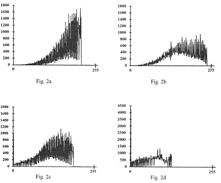
As the gradient with sx s neighborhoodfor a point p represents the local aspect, the statistics of gradients in an image should reveal its texture information. The occurrence distribution ofgradients will

be called the Morphological Gradient Texture Spectrum (MGTS), with the abscissa indicating the

gradient value and the ordinate representing its occurrence frequency.

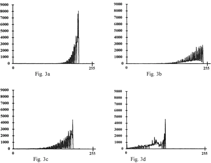
Fig. 2 and Fig. 3 showthe MGTS for the four images of Fig. 4 to Fig. 7 with 3 x 3 and 5x5

neighborhood respectively. In Fig. 2, we can find that the MGTS are distinguishable from each other. Thus, we can use them as a discriminating tool in texture classification. In addition, we can obtain the information about the size of basic texture unit in test images frOm the texture spectra. For instance, an abrupt peak appears in the spectrum shown in Fig. 3a which indicates the size of the constituting texture unit in Fig. 4a is near to the size of neighborhood used in creating the MGTS.

4500 4000 3500 3000 2500 2000 1500 1000 500 0

Fig. 2a-2d: Four MGTS for the four images shown in Fig. 4a-4d,

for each point.

SPIE Vol.2308 / 801 1800 1600 1400 1200 1000 800 600 400 200 0 0 1800 1600 1400 1200 1000 800 600 400 200 0 255 0 Fig. 2a Fig. 2b

H-255 255 1800 1600 1400 1200 1000 800 600 400 200 0 Fig. 2c 0 ₂₅₅ Fig. 2d

9000 9000 8000 8000 7000 7000 6000 6000 5000 5000 4000 4000 3000 3000 2000 2000 1000 1000 0 0 0 Fig. 3b 9000 9000 8000 ₈₀₀₀ 7000 ₇₀₀₀ 6000 6000 5000 5000 4000 4000 3000 3000 2000 2000 10000 10000 255 Fig. 3d

Fig. 3a-3d: Four MGTS for the four images shown in Fig. 4a-4d ,_{respectively,using 5x5 neighborhood}

for each point.

3. TEXTURE CLASSIFICATION

To demonstrate the discrimination performance of the MGTS, we use a supervised classification with minimum distance rule to classify nature images extracted from Brodatz's 12 _{These natural}

images are of size 256x256 with 256 gray levels. In our experiments, four different mosaics each contains four texture images are used and illustrated in Fig. 4 to Fig. 7. For each test mosaic, the

following algorithm is performed to classify the mosaic into one ofthe four classes.

step 1 : Randomly select a 30x30 sample subimage from each texture image;

step 2:

Calculate MGTS for each sample subimage using s x s neighborhood. The four

spectra are denoted as S(ij), where i= 1 to 4 and S(ij)

represents the

occurrence frequency of gradient valuej in the MGTS of the sample subimage i.

0

Fig. 3a

0

step 3:

Scan the four textures in the test mosaic by moving a 30x30 window across the

textures overlay. Calculate the MGTS of image masked by each window and

denoted as W(j),j=O to 255.

step 4:

Calculate the absolute difference between the MGTS of each window and one of

each sample:

255

D(i)

=

W(j)—S(i,j)

I =1,2,3,4 (1)

step 5: The central pixel of window considered will be assigned to class K such that

D(K)isminimum among all D(i).

Using the above described method, 232324 =(512—

30)2 pixels

of a test mosaic have been

processed and the test mosaic is assigned to one of the four classes. Results of the supervised

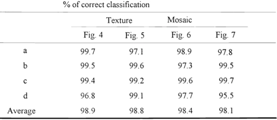
classification are listed in TABLE 1. An average classification accuracy rate of 98% is obtained using

the proposed method. Noted that the misclassification occurs mainly at the texture borders. If we

remove these pixels from our consideration, the correct classification rate will be near 100%.

a

b

a

b

Fig.4.

c d c d

FigS.

a b a b

Fig. 6

Fig. 4 to Fig. 7:

Fig. 7

Four texture mosaics each contains four Brodatz' texture images.

c d c d

TABLE 1: Results of classification using the proposed method.

% of correct classification

Texture Mosaic

Fig.4 Fig. 5 Fig. 6 Fig. 7

a

₉₉₇

97.1 98.9 97.8

b 99.5 99.6 97.3 99.5

c

99.4 99.2 99.6 99.7

d 96.8 99.1 97.7 95.5

4. VISUAL-PERCEPTUAL FEATURES EXTRACTION FROM MGTS

4.1. Texture Coarseness

The textural coarseness of a region is inversely related to the summation of texture gradients per

unit area in the 13 _{To extract coarseness feature from a texture, we can estimate the mean}

brighness of its corresponding MTGS. The larger the mean value, the finer the texture is. Let 4(i) (

1=0,..., 255) be the MGTS ofan image and A be the area ofthe image ( the total number ofpixels in the

image). The occurrence probability of intensity i in the spectrum is computed as

(2) In our study, we define the measurement of coarseness of a texture image as

CRS = ₍₃₎

ixp(i)

where c is a normalizing factor. From this definition, a coarser image will have a larger value of CRS. Fig. 8 illustrates the measure of coarseness for Brodatz' texture image D54 and the magnified image of D54, respectively. Here, we choose c=512. It can be found that the left image is larger than the other

one and gives a larger CRS.

C

CRS=4.53 CRS=1O.16

Fig. 8. Texture coarseness feature extraction from MTGS.

4.2. Texture Directionality

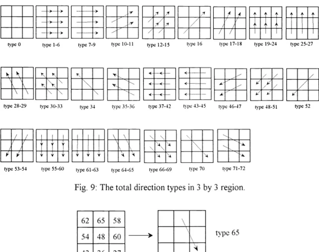
The directionality is detected from the histogram of texture gradient directions. Let R be a nv<nz

image square. The texture gradient direction in R can be described by a vector ' P1P2 ,wherethe

points p1 and p2 own the maximum and minimum gray values ofR, respectively. Fig. 9 illustrates all the possible texture direction types using 3 x3 _{image square. An example to transform an image square into}

the direction type is described in Fig. 10. Then, we can create a texture direction spectrum with the

abscissa indicating the direction types and the ordinate representing its occurrence frequency.

Fig. 1 1 illustrates the direction spectra for Brodatz' texture image D 5 and D3 7, respectively. We

can find the most two abrupt peaks of the left spectrum at direction type 45 and 9, respectively. It

means that the texture image D 1 5 has high frequent variation in the horizontal directions. Therefore, we can predict that there exists many vertical edges in D 1 5 .Incontrast, we can also predict the horizontal

edge feature for D54 by observing its direction texture spectrum.

M HE1

4:

H //

H

type0 type 1-6 type 7-9 1)Ve 10-11 type 12-15 Y1) 16 tYPe 17-18 type 19-24 type 25-27

[\\

hN\\L H 4':

H J//j/

type28-29 type 30-33 type 34 type 35-36 t''pe 37-42 Y1)C 43-45 t1)C46-47 type 48-51 type 52

H'HU

type53-54 type 55-60 type 61-63 type 64-65 type 66-69

Fig. 9: The total direction types in 3 by 3 region.

62 65 58

54 48 60

type 65

43 36 27

Fig. 10: An example to transform a 3 by 3 image block into the corresponding direction type.

Fig. 1 1 : The texture direction spectra for texture image D 1 5and_{d3 7, respectively.}

5. CONCLUSION

The texture spectrum method has been recently proposed for texture analysis. However, the original

method which uses texture units is very time consuming in texture classification. In this paper, we

extract the gradient feature from an image and create the corresponding texture spectrum for the image.

The texture spectrum is then used as a discrimination tool in texture analysis and classification. Experimental results show that our method is efficient in the texture classification. In addition, we

extract two visual-perceptual features from MTGS.

From the experimental results, we can conclude that MGTS is an excellent discriminating tool in

texture analysis and classification.

6. ACKNOWLEDGMENTS

This paper is partially supported by National Science Council Taiwan, R.O.C., under grant NSC

SPIE Vol. 2308 I 807 82-0408-E-009-.43 0.

D5

7000 6000 5000 4000 3000 2000 1000 0 D3 7 4500 4000 1 3500 3000

IIIHu1It.iiIiiii IIIIIIIIltttIItIuIIIliultIIlI IlIllIlIleelt

iLjIctJ'kAv1'\tkf,&,

0 iiitiiiiuiiiiiiiiiiiiitti ii-iiiiiiioniiueiuiiiiuusiiuiiinei-nin

7. REFERENCES

1 . R. M. Haralick,' Statistical and structural approaches to textures," IEEE Proc. ,_{67, pp. 786-804,}

1979.

2. F. Tomita and S. Tsuji, Computer analysis ofvisual textures, Kiuwer Academic Publishers, 1990.

3.

B. Kartikeyan and A. Sarker,' An identification approach for 2-D autoregressive

models in describing textures," CVGIP, 53, pp. 121-13 1, 1991.

4. M. Hassner and J.

Sklansky," The use of Markov random fields as models for

texture," Coniput. Graphic Image Process., 12, pp. 357-370, 1980.

5.

_{L.S. Davis, S.A. Johns, and J.K. Aggarwal," Texture analysis using generalized}

co-occurrence matrices," IEEE Trans. PAMI, 1,pp. 25 1-259, 1979.

6.

_{B.B. Mandelbrot, The Fractal Geometry of Nature, San Francisco, CA: Freeman,}

1982.

7.

S. Peleg, J. Naor, R. Hartley, and D. Avnir," Multiple resolution texture analysis

and classification," IEEE Trans. PAMI, 6, pp. 518-523, 1984.

8.

D. C. He and L. Wang, "

Texture

classification using texture spectrum." Pattern

Recognition. 23, pp. 905-910, 1990.

9.

D. C. He and L. Wang, "

_{Detecting texture edges from images." Pattern Recognition.}

25, pp. 595-600, 1992.

10. D. C. He and L. Wang, "

Tetxure

unit, texture spectrum and texture analysis." IEEE

Trans. on Geosicence and Remote Sensing 28, pp. 509-512, 1990.

11. 5.

_{Beucher, Segmentation d'images et morphologi'e mathematique, Ph.D.}

thesis, Ecole des Mines de Paris, June, 1990.

12. P. Brodatz, Textures: A photographic album for

artists and designers. Reinhold,

New York, 1968.

13. A. Rosenfeld, "

A

note on automatic detection on texture gradients "

IEEE Trans. 017