行政院國家科學委員會專題研究計畫 成果報告
多輸入多輸出有限脈衝系統的盲判別與對等化(3/3)
計畫類別: 個別型計畫 計畫編號: NSC94-2213-E-009-010- 執行期間: 94 年 08 月 01 日至 95 年 07 月 31 日 執行單位: 國立交通大學電機與控制工程學系(所) 計畫主持人: 林清安 計畫參與人員: 陳益生 報告類型: 完整報告 報告附件: 出席國際會議研究心得報告及發表論文 處理方式: 本計畫可公開查詢中 華 民 國 95 年 10 月 11 日
行政院國家科學委員會補助專題研究計畫 成果報告
多輸入多輸出有限脈衝系統的盲判別與對等化
計畫類別:個別型計畫
計畫編號:
執行期間: 92 年 8 月 1 日至 95 年 7 月 31 日
計畫主持人:林清安
計畫參與人員:陳益生
成果報告類型:完整報告
成果報告附件:出席國際學術會議心得報告及發表之論文(三年三份)
處理方式:本計畫可公開查詢
執行單位:國立交通大學電機與控制工程學系(所)
中 華 民 國 95 年 10 月 5 日
NSC92-2213-E-009-085 NSC93-2213-E-009-041 NSC94-2213-E-009-010多輸入多輸出有限脈衝系統的盲判別與對等化
中文摘要
本報告針對多出入多輸出頻率選擇衰減之無線通信系統提出了三種通道盲蔽判別
的方法。 判別的方法是利用所估測出來的接收信號協方差矩陣
,
先計算出通道乘積矩陣
,
再對此通道乘積矩陣取特徵分解
,
即可求出通道脈衝響應矩陣。 所提出的方法都是利用
對傳送信號作不同的編碼方式所引發的循環穩態特性來求解問題。 我們分別考慮了以下
三種不同的編碼方式
: (1)
週期性編碼
, (2)
週期性編碼加補零
, (3)
補零。 對前兩種判
別方法
,
我們也設計了最佳的週期性編碼器。 我們的方法在正規均方差的表現上可與子
空間的方法相比
,
但只需要較少的計算量
,
同時判別條件也較為寬鬆
,
另外我們的方法
還可適用於發射器數目較接收器數目多或者少的情況。 數值模擬的結果顯示我們所提出
的方法對通道階數過估的情況具有相當的強健性。
關鍵詞
:
多出入多輸出通道
,
盲蔽判別
,
週期性編碼
,
有限脈衝響應
,
補零
,
單載波補
零傳輸系統
,
正交分頻多工系統。
Blind Identification and Equalization for
Multiple-input Multiple-output Finite Impulse
Systems
Abstract
We propose three blind identification algorithms for multiple-input multiple-output (MIMO) frequency selective fading wireless communication channels. The algorithms com-pute the channel product matrices from the estimated covariance matrix of the received data and then determine the channel impulse response matrix via an eigenvalue-eigenvector de-composition. The algorithms are all based on transmitter-induced cyclostationarity through precoding. Three precoding are considered: (i) periodic precoding, (ii) periodic precoding plus zero padding, and (iii) zero padding alone. The algorithms, with optimally designed periodic precoding, have normalized root-mean-squared error (NRMSE) performance com-parable with subspace methods but require less computation, allow a more relaxed iden-tifiability condition, and are applicable to general MIMO systems with more transmitters or more receivers. Simulation results show that the algorithms are reasonably robust with respect to channel order overestimation.
Key words: MIMO channels, blind identification, periodic precoding (modulation),
finite impulse response, zero padding, single carrier zero padding transmission systems, OFDM systems
Contents
1 Introduction 1
1.1 Research Objective . . . 1
1.2 Literature Survey . . . 2
1.3 Organization of the Report . . . 3
2 Identification of General MIMO Channels 4 2.1 System Model and Formulation . . . 4
2.2 Blind Channel Identification . . . 6
2.2.1 The Identification Method . . . 6
2.2.2 Channel Order Overestimation . . . 9
2.2.3 More Transmitters Than Receivers . . . 10
2.3 Optimal Design of the Precoding Sequence . . . 10
2.3.1 Optimality Criterion . . . 10
2.3.2 On Selection of m . . . . 12
2.4 Identification Algorithm . . . 13
2.5 Simulation Results . . . 14
3 Identification of MIMO Single Carrier Zero Padding Channels 22 3.1 System Model and Formulation . . . 22
3.2 Blind Channel Identification . . . 24
3.2.1 The Identification Method . . . 24
3.2.2 Optimal Design of the Precoding Sequence . . . 27
3.2.3 Computation of G−10 . . . 29
3.2.4 Identification Algorithm . . . 30
3.3 Channel Equalization . . . 30
3.4 Simulation Results . . . 31
4 A Simplified Identification Algorithm for MIMO Zero Padding Channels 38 4.1 System Model and Formulation . . . 38
4.2 Blind Channel Identification . . . 39
4.2.2 Identification Algorithm . . . 43
4.2.3 Extension to MIMO Zero-Padding OFDM Systems . . . 43
4.3 Simulation Results . . . 44
5 Conclusions 50 Appendix 51 A Proof of Proposition 4.1 and 4.2 . . . 51
B The Eigenvalues of NTjNj for m = N − L . . . . 53
C A Proof of ∂f (α,β)∂α > 0 . . . . 54
D A Proof of Proposition 3.1 . . . 55
Biblography 56
Chapter 1
Introduction
1.1
Research Objective
Multiple-input multiple-output (MIMO) communication systems employing multiple transmit and receive antennas have received much attention due to the potential improve-ment in data transmission rate and link reliability they can offer. However, to exploit the potential advantage of MIMO systems, accurate channel state information is required. Channel can be identified or estimated using training signal which requires additional band-width. As a means to eschewing the need of training signal and the associated bandwidth requirement, blind identification of MIMO channels has been the focus of much research. Many blind identification algorithms have been proposed in recent years (see [1, 2] for a detailed review).
Existing algorithms for blind identification of MIMO finite impulse response (FIR) channels can be classified into second-order statistics methods [8]-[12],[20]-[22], higher-order statistics methods [3]-[5], and deterministic methods [6, 7]. Among these three types of methods, blind identification based on second-order statistics has been widely studied because it requires fewer data samples than the high-order statistics approach and it avoids poor estimation accuracy under low SNR, a common shortcoming of deterministic methods. Existing second-order statistics methods for MIMO systems, e.g., the subspace methods [8, 9], [26], [28]-[29], the linear prediction methods [10]-[12], and the matrix outer product decomposition methods [20]-[22], either impose restrictive assumptions on the channel to be identified or require large amount of computations, that may not be realistic in practical applications.
that are simple in computation and less restrictive in assumptions. It is hoped that the algorithms developed are thus more practical from an application point of view.
1.2
Literature Survey
It is well-known that cyclostationarity of the received data is the key to all blind iden-tification based on second-order statistics [1, 2]. Cycloststionarity can be induced either at the receiver, by oversampling or multiple antennas, or at the transmitter, by various coding methods. An advantage of transmitter-induced cyclostationarity is that the result-ing identification methods require less restrictive assumption on the channel, for example, channels with nonminimum phase zeros can be handled. One effective way to induce cy-clostationarity at the transmitter is by periodic precoding. Blind identification methods for general MIMO FIR channels using periodic precoding are found in [17, 18]. In [17], Chevreuil and Loubaton proposes a scheme that multiplies the input sequence by a constant modulus complex exponential precoding sequence to induce conjugate cyclostationarity at the transmitter. The scheme reduces the MIMO channel identification problem to several SIMO ones, which are then solved by the subspace method [24]. Each SIMO channel is required to be free from common zeros. However, the method in [17] allows only real input symbols and the identifiability condition is irreducible and column reduced. B¨olcskei et. al. [18] proposes a method for identifying each of the scalar channels individually up to a phase ambiguity using non-constant modulus periodic precoding sequences. The method imposes no restriction on channel zeros and is insensitivity to channel order overestimation. However, no systematic procedure for the design of the precoding sequences is given. In this report, we propose an identification method based on periodic precoding, which allows complex input symbols and gives an optimal design of the precoding sequence.
Single carrier zero padding (SC-ZP) block transmission systems, another communication systems, are used to remove interblock interference (IBI) [13, 14, 25, 26]. In the literature, to the best of our knowledge, there is only one paper, by Zeng and Ng [26], that proposes a subspace method for blind identification of MIMO SC-ZP block transmission systems. The method can be used to identify the channel impulse response matrix up to a matrix ambiguity when the channel is irreducible and the channel noise is uncorrelated and white. In this report, we first propose an identification method for MIMO SC-ZP systems based on periodic precoding, which can further relax the identifiability condition and reduce the computational load, compared with the method in [26]. In addition, we also propose another simplified identification method for such systems without periodic precoding. This simplified method can also apply to MIMO zero padding orthogonal frequency division multiplexing (ZP-OFDM) systems.
1.3
Organization of the Report
The report is organized as follows. In Chapter 2, we propose a blind identification method for general MIMO FIR channels based on periodic precoding. We also discuss the optimal design of the precoding sequence which takes into account the effect of additive channel noise and numerical error. We also propose a blind identification method for MIMO FIR channels in SC-ZP block transmission systems based on periodic precoding and discuss the optimal design of the precoding sequence in Chapter 3. In Chapter 4, we first propose a blind identification for SC-ZP block transmission systems without periodic precoding. Extension of this method to ZP-OFDM systems is given subsequently. Chapter 5 concludes this report and discusses the related future research.
We define the following operations that will be used in the derivation of the main result. First, for any m×m matrix A = [ak,l]0≤k,l≤m−1, define Γj(A) = [a0,j a1,j+1 · · · am−1−j,m−1]T
for 0≤ j ≤ m − 1, i.e., Γj(A) is the vector formed from the jth super-diagonal of A.
Sec-ond, for any J n× Jn matrix B = [Bk,l]0≤k,l≤n−1, where Bk,l is a block matrix of dimension
J × J, define Υj(B) = [BT0,j BT1,j+1 · · · BTn−1−j,n−1]T for 0≤ j ≤ n − 1, i.e., Υj(B) is the
Chapter 2
Identification of General MIMO
Channels
In this chapter, we propose a blind identification method for MIMO FIR channels based on periodic precoding. It is shown that, by properly choosing the precoding sequence, the MIMO FIR transfer functions, with K inputs and J outputs, can be identified up to a uni-tary matrix ambiguity. The transfer functions need not be irreducible or column reduced, and there can be more outputs (J ≥ K) or more inputs (J < K). The method exploits the linear relation between the covariance matrix of the received data and the “channel product matrices”. The method is shown to be robust with respect to channel order overestima-tion. The proposed algorithm requires solving linear equations and computing the nonzero eigenvalues and eigenvectors of a Hermitian positive semidefinite matrix. The performance of the algorithm, and indeed the identifiability, depends on the choice of the precoding se-quence. We propose a method for optimal selection of the precoding sequence which takes into account the effect of additive channel noise and numerical error in covariance matrix estimation. Simulation results are used to demonstrate the performance of the algorithm.
2.1
System Model and Formulation
We consider the linear MIMO baseband model of a communication channel with K transmitters and J receivers shown in Figure 2.1, where each source symbol sequence is multiplied by a P -periodic sequence, p(n), before transmission. The transmitted signal is
-N? -s1(n) p(n) u1(n) .. . ... -N? -sK(n) p(n) uK(n) MIMO FIR Channel -L? -t1(n) w1(n) x1(n) .. . ... -L? -tJ(n) wJ(n) xJ(n)
Figure 2.1. An MIMO channel model
where p(n + P ) = p(n), ∀ n. The discrete time model describing the relation between the transmitted signal uk(n) and the received signal xj(n) has the form of an MIMO FIR filter
with additive noise:
xj(n) = K X k=1 Ljk X l=0 hjk(l)uk(n− l) + wj(n), j = 1, 2,· · · , J, (2.2)
where hjk(0), hjk(1), · · · , hjk(Ljk), are the impulse responses of the channel between the
kth transmitter and the jth receiver, and wj(n) is the channel noise seen at the input of
the jth receiver. The equations (2.1) and (2.2) can be written more compactly as
u(n) = p(n)s(n), x(n) =
L
X
l=0
H(l)u(n− l) + w(n), (2.3)
where u(n), s(n) ∈ CK, and x(n), w(n) ∈ CJ are vector signals formed by stacking the respective scalar signals together, e.g., x(n) = [x1(n) x2(n) · · · xJ(n)]T. The jkth element
of H(l)∈ CJ×K is hjk(l), and L = maxj,k{Ljk} is the order of the MIMO channel. Thus
H(L)6= 0J×K.
Group the sequence of x(n) as ¯x(n) = [x(P n)T, x(P n + 1)T, · · · , x(P n + P − 1)T]T ∈ CKP, and let ¯w(n), ¯u(n), ¯s(n) be similarly defined, we have
¯
x(n) = H0¯u(n) + H1¯u(n− 1) + ¯w(n), (2.4)
where H0 is an J P × KP block lower-triangular Toeplitz matrix with [H(0)T H(1)T · · · H(L)T 0T
J×K · · · 0TJ×K]T ∈ CJ P×K as its first block column (i.e., the first K columns),
and H1 is an J P× KP block upper-triangular Toeplitz matrix with [0J×K · · · 0J×K H(L)
H(L− 1) · · · H(1)] ∈ CJ×KP as its first block row (i.e., the first J rows). Since p(n)
is periodic, ¯u(n) = G¯s(n) for all n, where G = diag[p(0)IK, p(1)IK,· · · , p(P − 1)IK] ∈
RKP×KP is a diagonal matrix, (2.4) can be written as
¯
x(n) = H0G¯s(n) + H1G¯s(n− 1) + ¯w(n), (2.5)
We assume that the receivers are synchronized with the transmitters. In addition, the following assumptions are made throughout this chapter.
(A1) s(n) and w(n) are white zero-mean vector sequences, and s(n) and w(n) are
tempo-rally and spatially uncorrelated. More precisely, E[s(k)s(j)∗] = δ(k− j)IK ∈ RK×K,
E[w(k)w(j)∗] = δ(k− j)σ2
wIJ ∈ RJ×J, E[s(k)w(j)∗] = 0K×J,∀ k, j, where δ(·) is the
Kronecker delta function.
(A2) An upper bound ˆL of the channel order L is known and the period P > ˆL + 1.
(A3) The channel impulse response matrix H = [H(0)T H(1)T · · · H(L)T]T is full
col-umn rank, i.e., rank(H)=K.
In the next section, we will derive an algorithm for blind identification of the MIMO channel impulse response matrix H using second-order statistics of the received data.
2.2
Blind Channel Identification
In this section, we derive the proposed method for the case under assumptions (A1), (A2), (A3) and noiseless case. We show that by appropriately selecting the periodic precoding sequence, any MIMO channel satisfying (A3) is identifiable up to an K × K unitary matrix ambiguity. The effect of noise and optimal design of the precoding sequence are discussed in Section 2.3.
2.2.1
The Identification Method
We first derive the proposed method for the case where the channel order L is known with P > L + 1, there are more receivers, i.e., J ≥ K, and the noise is absent. We discuss the cases of channel order overestimation and more transmitters than receivers (i.e., K > J ) in Section 2.2.2 and 2.2.3, respectively.
From (2.5) and assumption (A1), the covariance matrix of ¯x(n) can be written as
(noiseless case)
Rx¯ = E[¯x(n)¯x(n)∗] = H0G2H∗0+ H1G2H∗1. (2.6)
Let J∈ RP×P be the matrix whose first sub-diagonal are all one, i.e., Γ
1(JT) = [1 1 · · · 1]T ∈ R(P−1), and all remaining entries are zero. The block Toeplitz structures of H
0 and H1 allow us to write H0 = PL k=0J k ⊗ H(k) and H 1 = PL k=0(J T)P−k ⊗ H(k), respectively.
written as H0G2H∗0 = PL k=0Jk⊗ H(k) ¡ G2 p⊗ IMt ¢ PL l=0 ¡ Jl⊗ H(l)¢∗ = PLk=0PLl=0¡Jk⊗ H(k)¢ ¡G2 p⊗ IMt ¢ ¡ (JT)l⊗ H(l)∗¢ = PLk=0PLl=0¡JkG2 p(JT)l ¢ ⊗ (H(k)H(l)∗) , (2.7)
where we have used the identies (A⊗B)∗ = A∗⊗B∗ and (A⊗B)(C⊗D) = (AC)⊗(BD) [35, p.190]. Similarly, H1G2H∗1 can be written as
H1G2H∗1 = L X k=0 L X l=0 ¡ (JT)P−kG2pJP−l¢⊗ (H(k)H(l)∗) . (2.8)
The following proposition shows that the matrices JkG2
p(JT)land (JT)P−kG2pJP−lhave
special structures that allow decomposition of (2.6) into a group of decoupled equations. Roughly speaking, the jth block super-diagonal part of (2.6) involves only the unknown “channel product matrices”, H(k)H(k +j)∗, k = 0, 1,· · · , L−j. For example, the equations corresponding to the diagonal blocks (j = 0) involve only H(k)H(k)∗, k = 0, 1,· · · , L. In the proposed identification algorithm, these “channel product matrices” are computed first by solving linear equations, and then the channel impulse response matrices H(k) are computed via eigenvalue-eigenvector decomposition.
Proposition 2.1 : Let 0≤ k, l ≤ L be two non-negative integers. Then
(a) For l = k + j, where 0≤ j ≤ L − k, both JkG2
p(JT)l and (JT)P−kG2pJP−l are upper
triangular matrices with only the respective jth upper diagonals nonzero, and Γj ¡ JkG2p(JT)l¢ = [0| {z }· · · 0 k entries p(0)2 p(1)2 · · · p(P − 1 − k − j)2 | {z } P−k−j entries ]T, (2.9) Γj ¡ (JT)P−kG2pJP−l¢= [p(P − k)2 p(P − k + 1)2 · · · p(P − 1)2 | {z } k entries 0 · · · 0 | {z } P−k−j entries ]T. (2.10) (b) For l < k, both Γj ¡ JkG2 p(JT)l ¢ and Γj ¡ (JT)P−kG2 pJP−l ¢
are lower triangular with zero diagonal matrices.
Proof : See [16].
It follows from (2.9) and (2.10) that Γj ¡ JkG2p(JT)l¢+ Γj ¡ (JT)P−kG2pJP−l¢ = [p(P − k)2 · · · p(P − 1)2 | {z } k entries p(0)2 · · · p(P − 1 − k − j)2 | {z } P−k−j entries ]T if j = l− k ≥ 0 0(P−j)×1 if j 6= l − k . (2.11)
Since Υj ¡¡ JkG2p(JT)l¢⊗ H(k)H(l)∗¢= Γj ¡ JkG2p(JT)l¢⊗ H(k)H(l)∗ (2.12) and Υj ¡¡ (JT)P−kG2pJP−l¢⊗ H(k)H(l)∗¢ = Γj ¡ (JT)P−kG2pJP−l¢⊗ H(k)H(l)∗, (2.13) it follows from (2.6)-(2.8) and (2.11)-(2.13) that Υj(R¯x) can be derived as follows.
Υj(R¯x) = Υj ¡ H0G2H∗0+ H1G2H∗1 ¢ =PLk=0PLl=0Υj ¡¡ JkG2 p(JT)l ¢ ⊗ (H(k)H(l)∗)¢+ Υ j ¡¡ (JT)P−kG2 pJP−l ¢ ⊗ (H(k)H(l)∗)¢ =PLk=0PLl=0{Γj ¡ JkG2 p(JT)l ¢ + Γj ¡ (JT)P−kG2 pJP−l ¢ } ⊗ H(k)H(l)∗ =PLk=0−j[p(P − k)2 · · · p(P − 1)2 p(0)2 · · · p(P − 1 − k − j)2]T ⊗ H(k)H(k + j)∗ =PLk=0−j[p(P − k)2I J · · · p(P − 1)2IJ p(0)2IJ · · · p(P − 1 − k − j)2IJ]TH(k)H(k + j)∗ (2.14) The right hand side of (2.14) is a linear combination of block columns with the channel product matrices, H(k)H(k + j)∗, as coefficients. If we define, for 0≤ j ≤ L,
Fj = [(H(0)H(j)∗)T (H(1)H(j + 1)∗)T · · · (H(L − j)H(L)∗)T]T ∈ CJ (L−j+1)×J, (2.15)
then (2.14) can be written in a more compact form as
Υj(Rx¯) = MjFj ∀ 0 ≤ j ≤ L, (2.16) where Mj ∈ RJ (P−j)×J(L−j+1) is defined as Mj = p(0)2 p(P − 1)2 p(P − 2)2 · · · p(P − L + j)2 p(1)2 p(0)2 p(P − 1)2 · · · p(P − L + j + 1)2 p(2)2 p(1)2 p(0)2 · · · p(P − L + j + 2)2 .. . ... ... ... ... p(P − 3 − j)2 p(P − 4 − j)2 p(P − 5 − j)2 · · · p(P − L − 3)2 p(P − 2 − j)2 p(P − 3 − j)2 p(P − 4 − j)2 · · · p(P − L − 2)2 p(P − 1 − j)2 p(P − 2 − j)2 p(P − 3 − j)2 · · · p(P − L − 1)2 ⊗ IJ. (2.17) We note that Mj, 1≤ j ≤ L, is obtained from M0 by deleting its last jJ rows and last jJ columns.
Since P > L + 1, the (L + 1) equations in (2.16) are overdetermined and for the noise free case, these equations are consistent. We note that the matrix Mj, j = 0, 1,· · · , L, is
sequence, we can make each Mj full column rank. Then the solution Fj can be obtained
as
Fj = (MTjMj)−1MTjΥj(R¯x) . (2.18)
If Fj, 0 ≤ j ≤ L, are computed from (2.18), then we have the channel product matrices
H(k)H(l)∗ for 0 ≤ k ≤ l ≤ L. We now consider the computation required to determine the channel impulse response matrix H from Fj.
Let Q be the Hermitian matrix defined by Υj(Q) = Fj for j = 0, 1,· · · , L, and let the
channel impulse response matrix H = [H(0)T H(1)T · · · H(L)T]T. Clearly we have
Q = HH∗. (2.19)
Since rank(H) = K by assumption (A3), Q has rank K. Since Q is Hermitian and positive semidefinite, Q has K positive eigenvalues, say, λ1,· · · , λK. We can expand Q as
Q = K X j=1 (pλjdj)( p λjdj)∗, (2.20)
where dj is a unit norm eigenvector of Q associated with λj > 0. We can thus choose the
channel impulse response matrix to be b H = [pλ1d1 p λ2d2 · · · p λKdK]∈ CJ (L+1)×K. (2.21)
We note H can only be identified up to a unitary matrix ambiguity U ∈ CK×K [20, 21],
i.e., bH = HU, since bH bH∗ = HH∗ = Q. The ambiguity matrix U is intrinsic to methods for blind identification of multiple input systems using only second-order statistics [20, 21].
2.2.2
Channel Order Overestimation
So far we have assumed that the channel order L is known. If only an upper bound ˆ
L≥ L is available with P > ˆL + 1, then following the same process given in Section 2.2.1,
the corresponding J ( ˆL + 1)× J(ˆL + 1) matrix Q can be similarly constructed as in (2.19).
The last ( ˆL−L) block columns (i.e., (ˆL−L)J columns) of Q are zero, so are its last (ˆL−L)
block rows. Hence again, Q is of rank K and has K positive eigenvalues with the associated eigenvectors all of the form ˆd = [dT 0 · · · 0]T ∈ CJ ( ˆL+1)where d∈ CJ (L+1). Thus, we can determine the channel impulse response matrix, up to a unitary matrix ambiguity, from the K eigenvectors associated with the K positive eigenvalues of Q. In the noise free case, we can, in theory, also determine the actual channel order.
2.2.3
More Transmitters Than Receivers
In the above discussions, we assume that there are more receivers than transmitters, i.e., J ≥ K. If there are more transmitters, i.e., K > J, then either J(L + 1) ≥ K or
K > J (L + 1). If J (L + 1)≥ K, then H is a tall matrix and assumption (A3) is generically
satisfied [33]. Hence the proposed method still applies. If K > J (L+1), then rank(H) < K and assumption (A3) does not hold. Hence the proposed method is applicable to the more transmitters case, provided the additional condition J (L + 1) ≥ K is satisfied. We note that if the channel has more transmitters than receivers, channel equalization and source separation may be difficult even if accurate channel estimate is available. In addition, we note that in the proposed method, the channel impulse response matrix H is only assumed to be full column rank (A3). Hence the channel needs not be irreducible or column reduced.
2.3
Optimal Design of the Precoding Sequence
In Section 2.2, we see that in order to identify the channel, the precoding sequence must be selected so that the resulting matrix Mj is full column rank such that Fj can
be exactly solved as (2.18). However, when noise is present, the covariance matrix R¯x
contains the contribution of noise and numerical error is present in the estimation of R¯x
in practice. This implies that (2.16) usually has no solution and (2.18) becomes a least squares approximate solution. The choice of Mj will affect error in the computation of Fj
since different MT
jMj in (2.18) usually have different condition numbers. In this section,
we discuss the optimal design of the precoding sequence, which takes into account the effect of noise and numerical error in estimating ˆR¯x, so as to increase the accuracy of Fj and
thus reduce the channel estimation error.
2.3.1
Optimality Criterion
Now we consider the general case that noise is present and discuss the design of the precoding sequence p(n). From (2.4) and assumption (A1), the covariance matrix of the received signal is
R¯x = H0G2H0∗+ H1G2H∗1+ σ 2
wIJ ⊗ IP. (2.22)
From (2.22) and (2.6), we see that noise has only contribution to the diagonal entries of
except for the j = 0 group, which becomes Υ0(R¯x) = Υ0 ¡ H0G2H∗0+ H1G2H∗1 ¢ + σw2Υ0(IJ⊗ IP) = M0F0+ Y, (2.23) where Y = σ2
w[IJ IJ · · · IJ]T ∈ RJ P×J. Thus from (2.18), ˆF0, the least squares approxi-mation of F0, can be written by
ˆ
F0 = (MT0M0)−1MT0 (M| 0F{z0+ Y)} Υ0(R¯x(0))
= F0+ (MT0M0)−1MT0Y = F0+ Z, (2.24)
which is F0 plus a perturbation term due to noise. The perturbation term Z is the least squares solution of the equation M0Z = Y. We note that if every column of Y is orthogonal to every column of M0, then Z = 0, which implies ˆF0 = F0. But that is impossible since the entries of M0 are positive and those of Y are nonnegative. Therefore, we seek to appropriately choose the precoding sequence p(n) such that every column of Y is as close to being orthogonal to that of M0 as possible. To this end, we first define qki and yi shown
below as the columns of M0 and Y, respectively:
M0 = " q01 q02 · · · q0J | {z } M0(:,1:J ) q11 q12 · · · q1J | {z } M0(:,J +1:2J ) · · · q|L1 qL2{z· · · qLJ} M0(:,LJ +1:(L+1)J ) # , (2.25) Y = σw2[IJ IJ · · · IJ]T = [y1 y2 · · · yJ]. (2.26)
Then, due to the special structure of the block matrix M0 and Y, it is easy to check that
qki is orthogonal to yj, i.e., qTkiyj = 0 for j 6= i, e.g.,
qT01y2 = [p(0)| 2{z0 · · · 0} J entries · · · p(P − 1)2 0 · · · 0 | {z } J entries ][0 σw2 0 · · · 0 | {z } J entries · · · 0 σ2 w0 · · · 0 | {z } J entries ]T = 0, and each qT
kiyi assumes the same value, σw2
PP−1 n=0 p(n) 2, for k = 0, 1,· · · , L, i = 1, 2, · · · , J, e.g., qT01y1 = [p(0)| 2{z0 · · · 0} J entries · · · p(P − 1)2 0 · · · 0 | {z } J entries ][σ2w0 · · · 0 | {z } J entries · · · σ2 w 0 · · · 0 | {z } J entries ]T = σ2w P−1 X n=0 p(n)2.
Thus we only need to consider the relation between columns of q01 and y1 (the case of
k = 0 and i = 1). Define the correlation coefficient
γ = q
T
01y1
kq01k2ky1k2
. (2.27)
Since γ is nonnegative and by Cauchy-Schwarz inequality, 0≤ γ ≤ 1. In order to make the perturbation term Z small, we choose q01 so that the correlation coefficient γ is as small
as possible. Based on this point of view, we formulate the optimal selection problem as minimizing γ subject to 1 P P−1 X n=0 |p(n)|2 = 1, (2.28) |p(n)|2 ≥ τ > 0, ∀ 0 ≤ n ≤ P − 1. (2.29) Roughly, constraint (2.28) normalizes the power gain of the precoding sequence of each transmitter to 1; constraint (2.29) requires that at each instant, the power gain is no less than τ . Note that the problem of selecting the precoding sequence is identical to the SISO case considered in [16]. Thus the optimal precoding sequence p(n) is a two-level sequence with a single peak in one period [16]. More specifically, for each m, 0≤ m ≤ P − 1,
p(n) =
( p
P (1− τ) + τ , n = m √
τ , n 6= m, 0 ≤ n ≤ P − 1 (2.30)
is an optimal precoding sequence. Because the precoding sequence is periodic with period
P , the single peak can be placed at any one of the P positions which yield the same γ =
1
√
P (1−τ)2+τ (2−τ). Note that γ decreases as τ decreases, which implies that the noise effect in
the estimation of covariance matrix R¯x is minimized and thus identification performance
improves. However the peak location m does significantly affect the numerical condition of the linear equation (2.16). We discuss the selection of m next.
2.3.2
On Selection of m
We now consider the selection of m. We know that different choices of m result in dif-ferent matrix Mj and affect the numerical computation of Fj, j = 1, 2,· · · , L, in (2.18) and
ˆ
F0 in (2.24), since different MTjMj may have different condition number. If the condition
number is large, then the matrix MT
jMj is ill-conditioned and the computations in (2.18)
and (2.24) are sensitive to data error. Let
µ = max
0≤j≤Lκ(M
T
jMj), (2.31)
where κ(A) is the condition number of A. Our goal is to choose m so as to minimize the largest condition number of the corresponding matrices MTjMj, j = 0, 1,· · · , L. Since the
peak appears at one of the P possible positions in the periodic precoding sequence, there are P precoding sequences which may result in P different µ. The following result shows that some choices of m are to be avoided since they result in some Mj being rank deficient
Proposition 2.2 : At least one Mj, 0 ≤ j ≤ L, is not full column rank if and only if
P − L + 1 ≤ m ≤ P − 2.
Proof : See Appendix A.
Hence if we choose, either 0≤ m ≤ P − L or m = P − 1, then each Mj is full column
rank and the channel is identifiable. The following result shows that we can classify the remaining choices into 2 groups that are relevant to the optimal choice of m.
Proposition 2.3 :
(a) Each of the (P − L) choices, m = 0, m = 1, · · · , m = P − L − 1, results in the same µ denoted by µ1.
(b) The two choices m = P − L and m = P − 1 result in the same µ denoted by µ2. Also
µ2 ≥ µ1.
Proof : See Appendix A.
From Proposition 2.3, we know if µ2 > µ1, then we choose case (a); if µ2 = µ1, we proceed to compare the second largest condition numbers of the set of matrices{MT
jMj}Lj=0
for these two cases and choose the case whose value is smaller. If they are again equal, the same procedure can be done by comparing the third largest condition numbers and so on. Moreover, for 0 ≤ m ≤ P − L − 1 (case (a)), since the condition numbers of MT
jMj
are the same for each fixed j, j = 0, 1,· · · , L, (see Appendix A), we can use m = 0 to represent case (a). Similarly, m = P − 1 can be used to represent case (b). Hence the optimal selection of m reduces to one of two cases: m = 0 or m = P − 1. In other words, the optimal precoding sequence has a peak either at the beginning or at the end.
2.4
Identification Algorithm
So far, we have proposed a method for blind identification of FIR MIMO channels using periodic precoding sequence. It is shown that, by properly choosing the precoding sequence, the MIMO FIR transfer functions, with K inputs and J outputs, can be identified up to a unitary matrix ambiguity. The proposed algorithm requires solving linear equations and computing the nonzero eigenvalues and eigenvectors of a Hermitian positive semidefinite matrix. Since the cyclostationarity is induced at the transmitter, the identifiability condi-tion imposed on the channel is minimum: it only requires that channel impulse response matrix H is full column rank. The channel transfer matrix is not required to be irreducible or column reduced. The channel can have more receivers or more transmitters. The per-formance of the algorithm depends on the precoding sequence which is optimally designed to reduce the effect of noise and error in estimating the covariance matrix of the received data.
We summarize the proposed method as the following algorithm.
1) Use the precoding sequence p(n) in (2.30) with optimal selection of m = 0 or m = P− 1 to form the matrix Mj in (2.17).
2) Estimate the covariance matrix R¯x via the time average ˆR¯x = S1
PS
i=1¯x(i)¯x(i)∗, where
S is the number of data block (i.e., SP is the number of samples for each transmitter).
3) Compute Fj, formed by the channel product matrices, for j = 0, 1,· · · , L, using (2.18).
4) Form the matrix Q as in (2.19), and obtain the channel impulse response matrix (2.21) by computing the K largest eigenvalues and the associated eigenvectors of Q.
2.5
Simulation Results
In this section, we use several examples to demonstrate the performance of the proposed method. The channel normalized root-mean-square error (NRMSE) is defined as
NRMSE = 1 kHkF v u u t1 I I X i=1 k bH(i)− Hk2 F, (2.32)
where k · kF denotes the Frobenius norm. bH(i) = [ bH(i)(0)T Hb(i)(1)T · · · bH(i)(L)T]T is the
estimate of channel impulse response matrix H after removing the unitary matrix ambiguity by the least squares method [21]. I = 100 is the number of Monte Carlo runs. The input source symbols are independent and identically distributed (i.i.d.) QPSK signals. The channel noise is temporally and spatially white Gaussian. The signal-to-noise ratio (SNR) at the output is defined as SNR =
1 P PP−1 n=0E[kt(n)k22] E[kw(n)k2 2] , where t(n) = [t1(n) · · · tJ(n)] T is the
signal component of the received signal (see Figure 2.1). 1) Simulation 1 – optimal selection of precoding sequences In this simulation, we use the following model
H(z) = " 1.34− 0.55i 1.67 + 0.12i −0.69 + 0.25i −0.51 − 0.33i # | {z } H(0) + " −1.45 + 0.21i −1.35 + 0.21i 0.62− 0.31i −0.76 + 0.43i # | {z } H(1) z−1 + " −0.31 + 0.15i −0.41 − 0.16i −0.29 + 0.21i −0.25 − 0.14i # | {z } H(2) z−2 (2.33)
to demonstrate the effect of different precoding sequences on the performance of the pro-posed method. In experiment 1, the first sequence is chosen as {0.767 1.07 1.07 1.07}, which satisfies (2.28) and (2.29). The second and third sequences are chosen based on
(2.30) for P = 4 and τ = 0.5878 with the two possible peak positions: m = 0 and m = 3. By computation, the corresponding µ for the three cases are 40.0, 4.66 and 22.1, respec-tively. Thus m = 0 is the optimal selection. Figure 2.2 shows that for SNR=10 dB, there are about 5∼7 dB and 5∼9 dB difference in NRMSE between the optimal one and two others.
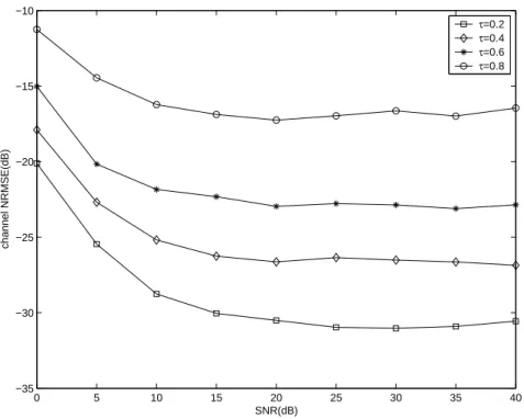
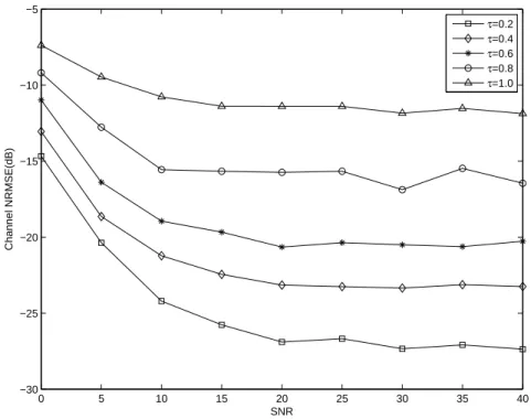
In experiment 2, we use the precoding sequences that satisfy (2.30) with m = 0, but with different τ to test the effect of τ on the identification performance. Figure 2.3 shows that for each sequence, when the number of samples (for each transmitter) is fixed at 1000, the NRMSE decreases as SNR increases and is roughly constant for SNR≥ 20 dB. A possible explanation is that for sufficiently large SNR, the NRMSE is contributed mainly by numerical error rather than by channel noise. Figure 2.3 also shows that the identification performs better for smaller τ , which is consistent with the conclusion at the end of Section 2.3.1.
2) Simulation 2 – channel order overestimation
In this simulation, we use the following channel model
H(z) = " 0.4851 0.3200 −0.3676 0.2182 # | {z } H(0) + " −0.4851 0.9387 0.8823 0.8729 # | {z } H(1) z−1+ " 0.7276 −0.1280 0.2941 −0.4364 # | {z } H(2) z−2 (2.34) given in [19]. For each upper bound ˆL, 0 ≤ (ˆL − L) ≤ 6, we choose P = ˆL + 2, SNR=10
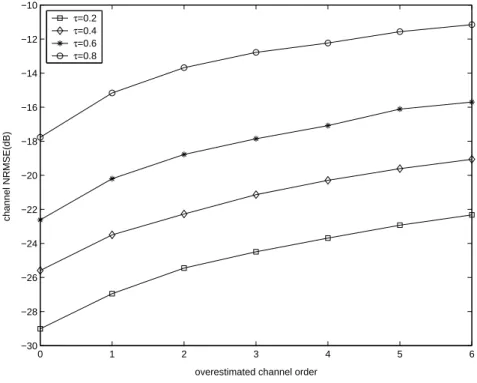
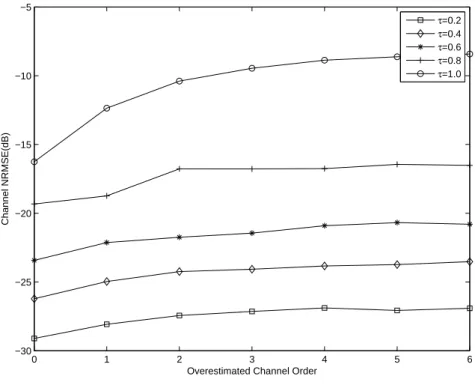
dB, and 1000 samples (for each transmitter) for simulation. The precoding sequences are chosen as (2.30) with m = 0 and τ = 0.2, 0.4, 0.6, and 0.8. Figure 2.4 shows the NRMSE increases with increasing channel order overestimation. We see the proposed method is quite robust to channel order overestimation when τ is small. For example, with τ = 0.4, when ( ˆL− L) increases from 0 to 3, the NRMSE increases from -25.5dB to -21dB, which
is still a low value.
3) Simulation 3 – a 3-input 2-output channel
In this simulation, we use the 3-input 2-output model
H(z) = " 1.6 0.88 0.66 0.8 0.44 0.33 # | {z } H(0) + " −0.44 0.35 0.14 −0.14 0.37 0.23 # | {z } H(1) z−1+ " 0.13 0.01 0.08 0.26 0.02 0.16 # | {z } H(2) z−2 (2.35) to illustrate the performance of the proposed method for channel with more transmitters than receivers. Note that H is full column rank, but the channel is not irreducible [21]
because H(0) is not full rank, and it is not column reduced [21] either because H(2) is not full rank. In experiment 1, the precoding sequences (P = 4) are given as in (2.30) with m = 0 and m = 3, respectively. Figure 2.5 shows that the NRMSE decreases as the number of data samples increases for SNR=10 dB. As expected, m = 0 case (the optimal selection) is better than m = 3 case.
In experiment 2, we use the precoding sequences that satisfy (2.30) with m = 0, but with different τ to test the effect of τ on the identification performance. Figure 2.6 shows that for each sequence, when the number of samples (for each transmitter) is fixed at 1000, the NRMSE decreases as SNR increases and is roughly constant for SNR ≥ 25 dB due to numerical error. Figure 2.6 also shows the identification performs better for smaller τ .
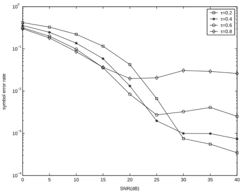
4) Simulation 4 – channel equalization performance
In this simulation, we use the channel model given in (2.34) to demonstrate the perfor-mance of the proposed method for channel equalization. We use the precoding sequences that satisfy (2.30) with m = 0, but with different τ to test the effect of τ on the equalization performance. For simplicity, we use the minimum mean square error (MMSE) equalizer. The equalizer is a 17-tap Wiener filter with 12-tap reconstruction delay whose jth output ˆ
uj(k) is an estimate of uj(k) for j = 1, 2,· · · , K. Since the precoding scheme is applied
at the transmitter, we need to multiply ˆuj(k) by the corresponding p(k)−1 to obtain an
estimate of sj(k) for j = 1, 2,· · · , K. The number of samples is 1200. We first identify the
channel using the first 400 samples and then do equalization. To obtain smoother curves, we use I = 300 as the number of Monte Carlo runs rather than 100.
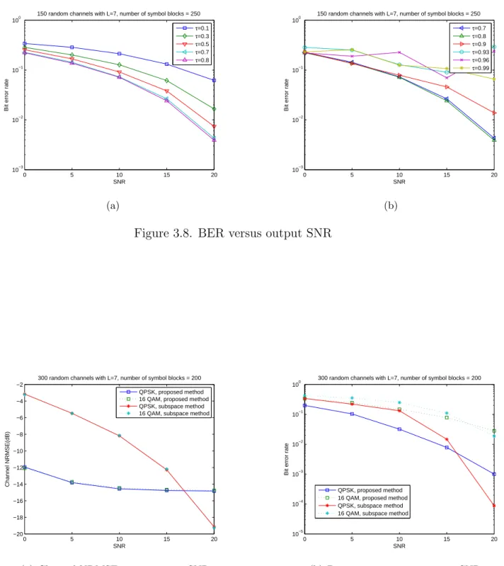
Figure 2.7 shows that under low SNR, the proposed method performs better when τ is large; however, under high SNR, the proposed method performs better when τ is low. A possible explanation is as follows.
Channel estimates become more accurate as τ becomes smaller, but the gains p(k)−1 = 1
√
τ, k = 1, 2,· · · , P −1 become larger and result in larger noise amplification at the receiver.
Both channel estimation error and channel noise contribute to the (maximum likelihood) detection performance, i.e., the symbol error rate. In the low SNR region, the detrimental effect of noise amplification outweighs the benefit of small estimation error; whereas in the high SNR region, accurate channel estimation weighs more than the noise amplification effect. Hence we choose a small τ when SNR is high and a large τ when SNR is low.
5) Simulation 5 – Comparisons with other methods
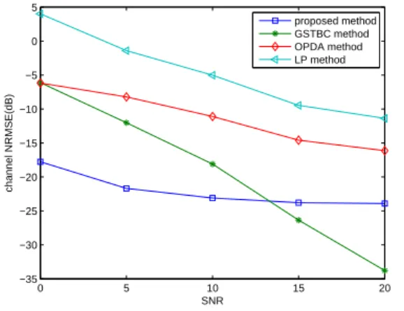
In this simulation, we generate 100 2-input 4-output random channels with order L = 2; each element in the channel impulse response matrix is a complex circular Gaussian random
variable with unit variance. We compare the proposed method with a generalized space time block codes (GSTBC)[23] based method. Both methods require periodic precoding sequences. For the proposed method, the precoding sequence is chosen as {1.500 0.767 0.767 0.767}; whereas the entries in the precoding sequence for the GSTBC method is chosen as random entries with modulus 1 for each random channel simulation [23]. The performance of the proposed method is also compared with a linear prediction (LP)[2, chap. 6] based method, and an outer product decomposition algorithm (OPDA)[20]. Both methods do not require a periodic precoder. MMSE equalizers are used for the proposed method, LP method, and OPDA method. For the GSTBC method, we use the customized equalizer proposed in [23]. Figure 2.8(a) shows that when the number of samples is 1200 (for each transmitter), the identification performance of the proposed method is better than those of the other three methods excepting the GSTBC method for SNR ≥ 13 dB. However, Figure 2.8(b) shows the equalization performance of the proposed method is only better than those of the LP and OPDA methods and worse than the GSTBC method. The inconsistency of the channel estimation and equalization performance of the proposed method and the GSTBC method for SNR≤ 13 dB may be due to the different precoding sequences and equalizers used. Figure 2.9 shows that when the number of samples is 200 (for each transmitter), the identification and equalization performance of the proposed method is better than that of the GSTBC method for SNR≤ 15 dB. Figure 2.9 shows that when the number of samples is small, the proposed method has better performance than the GSTBC method under low SNR.
100 200 300 400 500 600 700 800 900 1000 −22 −20 −18 −16 −14 −12 −10 −8 −6 Number of Samples Channel NRMSE(dB) m=0 m=3 non−optimal p(n)
Figure 2.2. Channel NRMSE versus number of samples
0 5 10 15 20 25 30 35 40 −35 −30 −25 −20 −15 −10 SNR(dB) channel NRMSE(dB) τ=0.2 τ=0.4 τ=0.6 τ=0.8
0 1 2 3 4 5 6 −30 −28 −26 −24 −22 −20 −18 −16 −14 −12 −10
overestimated channel order
channel NRMSE(dB)
τ=0.2
τ=0.4
τ=0.6
τ=0.8
Figure 2.4. Channel NRMSE versus ( ˆL− L)
100 200 300 400 500 600 700 800 900 1000 −22 −21 −20 −19 −18 −17 −16 −15 −14 −13 −12 number of samples channel NRMSE(dB) m=0 m=3
0 5 10 15 20 25 30 35 40 −30 −28 −26 −24 −22 −20 −18 −16 −14 −12 SNR(dB) channel NRMSE(dB) τ=0.2 τ=0.4 τ=0.6 τ=0.8
Figure 2.6. 3-input 2-output model: channel NRMSE versus output SNR
0 5 10 15 20 25 30 35 40 10−4 10−3 10−2 10−1 100 SNR(dB)
symbol error rate
τ=0.2
τ=0.4
τ=0.6
τ=0.8
0 5 10 15 20 −35 −30 −25 −20 −15 −10 −5 0 5 SNR channel NRMSE(dB) proposed method GSTBC method OPDA method LP method
(a) Channel NRMSE versus output SNR
0 5 10 15 20 10−6 10−5 10−4 10−3 10−2 10−1 100 SNR(dB)
symbol error rate
proposed method GSTBC method OPDA method LP method
(b) Symbol error rate versus output SNR
Figure 2.8. Comparison of NRMSE and symbol error rate, number of input samples = 1200 0 2 4 6 8 10 12 14 16 18 20 −22 −20 −18 −16 −14 −12 −10 −8 −6 −4 −2 SNR channel NRMSE(dB) proposed method GSTBC method
(a) Channel NRMSE versus output SNR
0 2 4 6 8 10 12 14 16 18 20 10−5 10−4 10−3 10−2 10−1 100 SNR(dB)
symbol error rate
proposed method GSTBC method
(b) Symbol error rate versus output SNR
Chapter 3
Identification of MIMO Single
Carrier Zero Padding Channels
In this chapter, we propose a blind identification method based on periodic precod-ing for another transmission systems, sprecod-ingle carrier with zero paddprecod-ing block transmission systems. The method uses periodic precoding on the source signal before transmission. The estimation of the channel impulse response matrix consists of two steps: (1) obtain the channel product matrix by solving a lower-triangular linear system and (2) obtain the channel impulse response matrix by computing the positive eigenvalues and eigenvectors of a Hermitian matrix formed from the channel product matrix. The method is applicable to MIMO channels with more transmitters or more receivers. A sufficient condition for identi-fiability is simply that the channel impulse response matrix is full column rank. The design of the precoding sequence which minimizes the noise effect in covariance matrix estimation is proposed and the effect of the optimal precoding sequence on channel equalization is discussed. Simulations are used to demonstrate the performance of the method.
3.1
System Model and Formulation
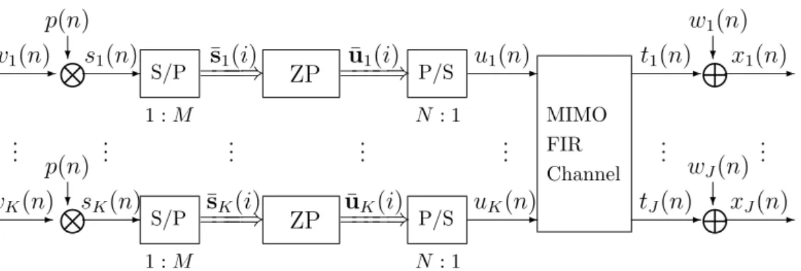
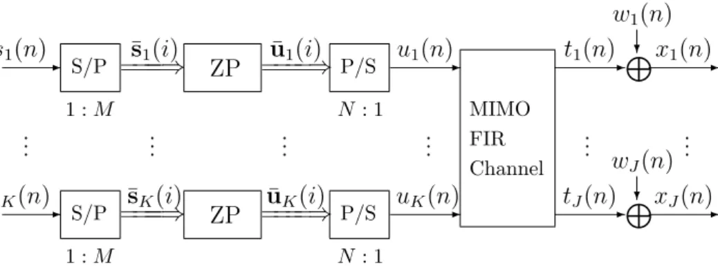
Consider the K-input J -output discrete time SC-ZP block transmission baseband model shown in Figure 3.1. At the transmitter, the kth input signal vk(n) is first multiplied by a
positive P -periodic sequence, p(n) ∈ R, to obtain sk(n) = p(n)vk(n), where p(n+P ) = p(n),
∀ n. Then sk(n) is passed through a serial-to-parallel block whose output is
-N? - S/P ====⇒ ZP ====⇒ P/S -v1(n) p(n) s1(n) ¯s1(i) u¯1(i) u1(n) 1 : M N : 1 .. . ... ... ... ... -N? - S/P ====⇒ ZP ====⇒ P/S -vK(n) p(n) sK(n) ¯sK(i) u¯K(i) uK(n) 1 : M N : 1 MIMO FIR Channel -L? -t1(n) w1(n) x1(n) .. . ... -L? -tJ(n) wJ(n) xJ(n)
Figure 3.1. An MIMO SC-ZP block transmission baseband model with periodic precoding
Then ¯sk(i) is passed through a zero padding prefilter F1 = [IM 0TP×M]T ∈ R(M +P )×M whose
output is
¯
uk(i) = F1¯sk(i) = [ ¯s| {z }k(i)T M entries 0· · · 0 | {z } P entries ]T = [u|k(iN )· · · uk{z(iN + M − 1)} M entries 0· · · 0 | {z } P entries ]T, (3.2)
where N = M + P . Finally, ¯uk(i) is converted to uk(n) via a parallel-to-serial block and
transmitted through the MIMO FIR channel. At the receiver, the jth received signal is
xj(n) = tj(n) + wj(n), where tj(n) is the signal component at the output and wj(n) is the
channel noise seen at the jth receiver. If we define x(n) = [x1(n) x2(n) · · · xJ(n)]T ∈ CJ,
then x(n) can be written as
x(n) =
L
X
l=0
H(l)u(n− l) + w(n) = t(n) + w(n), (3.3) where u(n) ∈ CK, w(n) ∈ CJ, and t(n) ∈ CJ are similarly defined as x(n), and H(l) ∈ CJ×K is the channel coefficient matrix whose jkth element h
jk(l), l = 0, 1,· · · , Ljk, is the
impulse response from the kth transmitter to the jth receiver, and L = maxj,k{Ljk} is the
order of the MIMO channel. We assume that H(L) 6= 0J×K. Group the sequence of x(n) as ¯x(i) = [x(iN )T x(iN + 1)T · · · x(iN + N − 1)T]T ∈ CJ N, and define ¯u(i) ∈ CKN and
¯
w(i) ∈ CJ N similarly as ¯x(i), we have ¯
x(i) = H0u(i) + H¯ 1¯u(i− 1) + ¯w(i), (3.4)
where H0 is a J N×KN block lower-triangular Toeplitz matrix with the first block column
being [H(0)T H(1)T · · · H(L)T 0TJ×K· · · 0TJ×K]T ∈ CJ N×K, and H1 is a J N × KN block
upper-triangular Toeplitz matrix with the first block row being [0J×K· · · 0J×K H(L) H(L−
1)· · · H(1)] ∈ CJ×KN. We assume that the receivers are synchronized with the transmit-ters. In addition, the following assumptions are made throughout this chapter.
(B1) The source signal v(n) = [v1(n) v2(n) · · · vK(n)]T ∈ CK is a zero mean white
se-quence with E[v(m)v(n)∗] = δ(m− n)IK ∈ RK×K, where δ(·) is the Kronecker delta
function. The noise is white zero mean with E[w(m)w(n)∗] = δ(m− n)σ2
wIJ ∈ RJ×J.
In addition, the source signal is uncorrelated with the noise w(n), i.e., E[v(m)w(n)∗] =
0K×J, ∀ m, n.
(B2) An upper bound ˆL of the channel order L is known, P = ˆL + 1, and M > P is a
multiple of P .
(B3) The channel impulse response matrix H = [H(0)T H(1)T · · · H(L)T]T is full column
rank, i.e., rank(H) = K.
In the next section, we derive an algorithm for blind identification of the MIMO channel impulse response matrix H using second-order statistics of the received data.
3.2
Blind Channel Identification
In this section, we derive the proposed method under assumptions (B1), (B2), and (B3). We discuss an optimal design of the precoding sequence, which takes into account the noise effect in the estimation of covariance matrix of the received data, so as to increase the accuracy in the computation of the channel product matrix HH∗ and thus reduce the channel estimation error. With the proposed optimal precoding sequence, the computation of HH∗ becomes particularly simple. Taking eigen-decomposition of HH∗, we obtain the channel impulse response matrix H up to a unitary matrix ambiguity.
3.2.1
The Identification Method
We first derive the proposed method for the case where the channel order L is known with P = L + 1, there are more receivers, i.e., J ≥ K, and the noise is absent. The cases of channel order overestimation and more transmitters than receivers (i.e., K > J ) are given at the end of this sub-section. The effects of noise and optimal design of the precoding sequence are discussed in Section 3.2.2.
From (3.4), we know that only the last L block columns of H1 are non-zero and zeros
are padded in the last P block rows of ¯u(i− 1) and ¯u(i) (see (3.2)). Hence the product H1u(i¯ − 1) equals the zero vector and (3.4) can be written as follows (noiseless case):
¯ x(i) z }| { x(iN ) .. . x(iN + L) .. . x(iN + M − 1) .. . x(iN + N − 1) = H0 z }| { H(0) .. . . .. H(L)· · · H(0) . .. ... ... H(L)· · · H(0) . .. ... . .. H(L)· · · H(0) ¯ u(i) z }| { u(iN ) .. . u(iN + L) .. . u(iN + M − 1) 0 ˙˙˙ 0 = He¯s(i), (3.5) where He is the sub-matrix formed from the first M block columns of H0 and ¯s(i) =
[u(iN )T u(iN + 1)T · · · u(iN + M − 1)T]T is the first M block entries of ¯u(i). Because
u(iN ) = [u1(iN ) u2(iN ) · · · uK(iN )]T (see the line below (3.3)) and uk(iN ) = sk(iM )
for k = 1, 2,· · · , K (see (3.2)), u(iN) = [s1(iM ) s2(iM ) · · · sK(iM )]T , s(iM).
Simi-larly, u(iN + m) = s(iM + m) for m = 1, 2,· · · , M − 1. Hence ¯s(i) = [s(iM)T s(iM +
1)T · · · s(iM + M − 1)T]T.
Let xf(i) = [x(iN )T x(iN + 1)T · · · x(iN + L)T]T be the first J (L + 1) rows of ¯x(i).
Then
xf(i) = Hfsf(i), (3.6)
where Hf ∈ CJ (L+1)×K(L+1) is the sub-matrix formed from the first (L + 1) block columns
and block rows of He, and sf(i) = [s(iM )T s(iM + 1)T · · · s(iM + L)T]T. Also we know
for k = 1, 2,· · · , K, sk(iM ) = p(iM )vk(iM ) = p(0)vk(iM ) from (3.1) and assumption
(B2). Hence s(iM ) = [p(0)v1(iM ) p(0)v2(iM ) · · · p(0)vK(iM )]T = p(0)v(iM ), where
v(iM ) = [v1(iM ) v2(iM ) · · · vK(iM )]T. Similarly, s(iM + n) = p(n)v(iM + n) for
n = 1, 2,· · · , L. Therefore (3.6) can be written as
xf(i) z }| { x(iN ) x(iN + 1) .. . x(iN + L) = Hp z }| { p(0)H(0) p(0)H(1) p(1)H(0) .. . ... . .. p(0)H(L) p(1)H(L− 1) · · · p(L)H(0) vf(i) z }| { v(iM ) v(iM + 1) .. . v(iM + L) . (3.7) Define S ∈ RJ (L+1)×J(L+1) as the matrix whose first block sub-diagonal entries are all I
J
(i.e., S(J + 1 : J (L + 1), 1 : J L) = IJ L), and all remaining entries are zero. Rewrite (3.7) as
Taking expectation of xf(i)xf(i)∗, we get the covariance matrix
Rf = E[xf(i)xf(i)∗] = HpH∗p . (3.9)
From (3.8), since Hp = [p(0)H p(1)SH · · · p(L)SLH], (3.9) can be written as
Rf = p(0)2HH∗+ p(1)2SHH∗ST +· · · + p(L)2SLHH∗(ST)L= L X k=0 p(k)2SkHH∗(ST)k. (3.10) From [37, p.414], we know that the general matrix equationPpj=1AjXBj = C can be
equiv-alently expressed as a matrix-vector equation form, hPpj=1BT
j ⊗ Aj
i
vec(X) = vec(C), where vec(·) is the vec-function which stacks up columns of a matrix. Hence the matrix equation (3.10) can be written in the following vector form:
vec(Rf) = vec à L X k=0 p(k)2SkHH∗(ST)k ! = à L X k=0 p(k)2Sk⊗ Sk ! vec(HH∗) = G· vec(HH∗). (3.11) Here G is a block Toeplitz lower-triangular matrix shown as follows:
G = L X k=0 p(k)2Sk⊗ Sk = p(0)2IJ F 0 · · · 0 p(1)2bS p(0)2IJ F · · · 0 .. . ... . .. ... p(L)2bSL p(L− 1)2bSL−1 · · · p(0)2I J F ∈ R F2×F2 , (3.12)
where F = J (L + 1) and bS ∈ RJ F×JF is a block diagonal matrix with S on the diagonal
blocks. Since G is square, the solution to (3.11) is
vec(HH∗) = G−1vec(Rf) (3.13)
provided p(0) 6= 0. We use the solution obtained in (3.13) to form a Hermitian matrix
Q = HH∗. Then under the assumption (B3), we can obtain the channel impulse response matrix, up to a unitary matrix ambiguity, by choosing the K largest eigenvalues and the associated eigenvectors of Q, like the way at the end of Section 2.2.1.
Remark 1: So far we have assumed that the channel order L is known. If only an upper
bound ˆL≥ L is available, then following the same process given in this sub-section, we
ob-tain vec(H\ovH∗ov) = [ PLˆ k=0Sk⊗ Sk]−1vec(Rf) where Hov = [H T 0 · · · 0 | {z } ˆ L−L blocks ]T ∈ CJ ( ˆL+1)×K.
Then we can also obtain Q = HovH∗ov. Note that the last ( ˆL−L) block columns and block
rows of Q are zero. Then similar to the discussion in Section 2.2.2, we can also identify the channel impulse response matrix.
Remark 2: The proposed method can apply to the case of more transmitters than
3.2.2
Optimal Design of the Precoding Sequence
When the noise is present, the covariance matrix Rf contains the contribution of noise.
Thus (3.9) becomes
Rf = E[xf(i)xf(i)∗] = HpH∗p+ σ
2
wIF, (3.14)
where F = J (L + 1). In this case, (3.11) becomes
vec(Rf) = G· vec(HH∗) + σw2vec(IF). (3.15)
From (3.13), the approximate solution of vec(HH∗) is \
vec(HH∗) = G−1vec(Rf). (3.16)
It follows from (3.16) and (3.15) that \
vec(HH∗) = vec(HH∗) + σ2wG| −1· vec(I{z F})
z
= vec(HH∗) + σw2z. (3.17)
The vector z = [z1z2 · · · zF2]T in (3.17) is the solution of Gz = vec(IF). Since the matrix
G is completely determined by the precoding sequence p(n), we seek to choose p(n) so that
kzk2
2 is minimized. To this end, we need to analyze the relations between z and p(n). By expanding the matrix equation Gz = vec(IF), we find that
p(0)2zi = 1 i = 1 + k(F + 1), k = 0, 1,· · · , J − 1 P1 n=0p(n) 2z i+(1−n)J(F +1) = 1 i = 1 + k(F + 1), k = 0, 1,· · · , J − 1 P2 n=0p(n) 2z i+(2−n)J(F +1) = 1 i = 1 + k(F + 1), k = 0, 1,· · · , J − 1 .. . ... ... PL n=0p(n)2zi+(L−n)J(F +1) = 1 i = 1 + k(F + 1), k = 0, 1,· · · , J − 1 (3.18)
and zj = 0 for all other indices j. We write (3.18) as the following matrix equation.
g0 0 · · · 0 g1 g0 · · · 0 .. . ... . .. ... gL gL−1 · · · g0 | {z } Gs m0 m1 .. . mL | {z } m = 1 1 .. . 1 | {z } y (3.19)
where Gs is a lower-triangular Toeplitz matrix, gn = p(n)2 for n = 0, 1,· · · , L, and mj =
zi+jJ (F +1)for j = 0, 1,· · · , L, i = 1+k(F +1), k = 0, 1, · · · , J −1. Hence Gz = vec(IF), the
relations between z and p(n), is reduced to (3.19), and minimization of kzk22 is equivalent to minimization ofkmk22, which is a nonlinear function of g0, g1,· · · , gL. Then the problem