利用紋理合成及形態學運算做彩色影像修補之研究

國

立

交

通

大

學

資訊科學與工程研究所

碩

士

論

文

利用紋理合成及形態學運算做彩色影像修補之研究

Color Image Inpainting using Texture Synthesis and

Morphological Operations

研 究 生：呂盈賢

指導教授：薛元澤 教授

利 用 紋 理 合 成 及 形 態 學 運 算 做 彩 色 影 像 修 補 之 研 究

Color Image Inpainting using Texture Synthesis and

Morphological Operations

研 究 生：呂盈賢 Student：Ying-Shian Lu

指導教授：薛元澤 Advisor：Yuang-Cheh Hsueh

國 立 交 通 大 學

資 訊 科 學 與 工 程 研 究 所

碩 士 論 文

A Thesis

Submitted to Institute of Computer Science and Engineering College of Computer Science

National Chiao Tung University in partial Fulfillment of the Requirements

for the Degree of Master

in

Computer Science June 2006

Hsinchu, Taiwan, Republic of China

利用紋理合成及形態學運算做彩色影像修補之研究

學生：呂盈賢

指導教授：薛元澤

國 立 交 通 大 學

資 訊 科 學 與 工 程 研 究 所

摘要

為了修補影像中受損的區域，或是移除影像中的某個物件，常常必須

使用影像修補的技術。因此如何有效且正確的修補一塊未知的區域便成為

一個重要的研究領域。本論文嘗試使用紋理合成及形態學運算來做影像修

補。實作上先使用數學形態學的 Opening 將受損區域分為兩大部分，其中

一部分是影像中受損極小的區域，另一部分則是受損範圍較大的區域。針

對受損極小的區域，計算周圍可用灰階值的平均值進行修補。而針對受損

範圍較大的區域，則尋找影像中最相近的紋理來修補，同時，應用 FFT 區

塊比對法去加速搜尋的時間。實驗結果顯示我們所提出的方法不僅能獲得

令人滿意的修補品質，且在運算的時間上是相當有效率的。

Color Image Inpainting using Texture Synthesis and

Morphological

Operations

student：Ying-Shian Lu

Advisors：Dr.Yuang-Cheh Hsueh

Institute of Computer Science and Engineering

College of Computer Science

National Chiao Tung University

ABSTRACT

Inpainting, techniques can repair damaged photographs and remove/replace selected objects on the image. The goals and applications of inpainting are numerous. How to effectively and correctly inpaint an unknown region has become an important research topic. In this thesis, we propose a new inpainting method by using texture synthesis and morphological operations. Based on mathematical morphology, we first use opening to split damaged regions into two parts. One consists of small damaged regions and the other consists of large damaged regions on the image. We inpaint the pixel in the small damaged regions by computing the average of undamaged neighboring pixels surrounding it. For the large damaged regions, we search the most similar texture to synthesize it. Simultaneously, we apply the FFT block matching algorithm to speedup the time of searching similar textures. The proposed method is computational efficient. Experimental results look “reasonable” to

誌謝

我在這裡要感謝我的指導教授 薛元澤教授，兩年來對我孜孜不倦的教

誨，教導我研究學問的方法及待人處世道理，讓我畢生受益無窮，以及我

的口試委員 張隆紋教授 與 莊仁輝教授，二位老師不吝指教，讓這篇論文

更加完善。

我還要感謝莊逢軒學長、何昌憲學長，給予我論文研究及寫作方面等

的各種建議，感謝江仲庭同學、劉裕泉同學、王慧縈同學、顏佩君同學、

林明志同學在這兩年內與我共同努力，互相砥礪，陪我度過這段快樂的實

驗室生活。

僅將此論文獻給我親愛的家人與朋友，我的父母及弟弟，感謝他們在

這段期間給我的關心、支持與鼓勵，祝福他們永遠健康快樂。

呂盈賢 謹誌於 國立交通大學資訊科學與工程研究所 中華民國九十五年六月

CONTENTS

ABSTRACT (CHINESE)...i

ABSTRACT (ENGLISH)...ii

ACKNOWLEDGEMENT...iii

CONTENTS ...iv

LIST OF FIGURES ...vii

LIST OF TABLES ...xi

CHAPTER 1 ...1

1.1 Motivation ...1

1.2 Related Works...3

1.3 Thesis Organization ...4

CHAPTER 2 ...6

2.1 Review of Digital Image Inpainting ...6

2.1.1 Image Inpainting Based on Partial Differential Equation (PDE) ...6

2.1.1.1 How to calculate

_I

n_t( ji, ) ? ...7 2.1.1.2 How to calculate

δ

_L

n( ji, ) ⎯→ ⎯ ? ...8 2.1.1.3 How to calculate ) , , ( ) , , ( n j i n j i

N

N

⎯→ ⎯ ⎯→ ⎯ ? ...9 2.1.1.4 How to calculate

∇

_I

n( ji, ) ? ...9

2.1.2 Fast Digital Image Inpainting...10

2.1.3 Texture Synthesis...12

2.1.4.2 How to calculate

n

p ?...17

2.1.4.3 How to calculate ∇

_I

⊥_p ? ...17

2.1.4.4 How to update confidence value ?...18

2.2 Block Matching ...19

2.2.1 SAD and SSD ...19

2.2.2 The FFT Block Matching Algorithm ...20

2.2.2.1 Resize input image to include a zero pad ...20

2.2.2.2 Windowed Sum Squared Table...21

2.2.2.3 Per-Block Convolution Sum...22

2.4 Mathematical Morphology ...24

2.4.1 Basic definition...25

2.4.2 Morphological operations...25

2.4.2.1 Dilation and Erosion...25

2.4.2.2 Closing and Opening ...26

2.4.3 Extension to Gray-Scale Images ...27

2.4.4 Morphological Gradient ...29

CHAPTER 3 ...31

3.1 Overview of Our Image Inpainting System...31

3.2 Splitting the damaged regions into several small and large parts...34

3.3 Using “Fast Digital Image Inpainting” to inpaint these small damaged parts ...36

3.4 Using “Priority Texture Synthesis” to inpaint these large damaged parts...39

3.5 Summation...40

CHAPTER 4 ...41

4.1 Experimental Environment...41

4.2.1 Comparison of inpainting results...43

4.2.2 Comparison of PSNR Values...56

4.2.3 Comparison of Running Time ...57

CHAPTER 5 ...59

5.1 Conclusions ...59

5.2 Future works...60

LIST OF FIGURES

Fig. 1- 1 Restoration of photographs...2

Fig. 1- 2 Removal of trees...2

Fig. 1- 3 Removal of a girl ...2

Fig. 1- 4 Removal of subtitles ...2

Fig. 1- 5 Applications of image coding...3

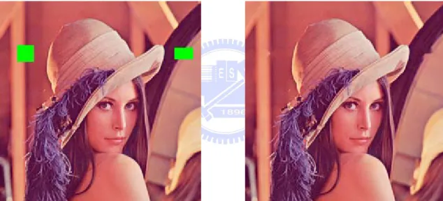
Fig. 1- 6 Special effects...3

Fig. 2- 1 The figure describes what is Isophote Directions ...7

Fig. 2- 2 Some gradient operators. (a) is Prewitt operator. (b) is Sobel operator...9

Fig. 2- 3 (top) Pseudocode for the fast inpainting algorithm. (bottom) Two diffusion kernels used with the algorithm... 11

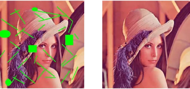
Fig. 2- 4 Removal of subtitles ... 11

Fig. 2- 5 Lena : (left) Picture with locally small damaged regions. (right) Restored image obtained with fast inpainting algorithm...12

Fig. 2- 6 Lena : (left) Picture with large damaged regions. (right) Restored image obtained with fast inpainting algorithm...12

Fig. 2- 7 Texture Synthesis Procedure ...13

Fig. 2- 8 Lena : (left) Picture with large damaged regions. (right) Restored image obtained with texture synthesis algorithm. ...14

Fig. 2- 9 The pseudocode of the exemplar-based texture synthesis algorithm. ...15

Fig. 2- 10 Structure propagation by exemplar-based texture synthesis. ...15

Fig. 2- 11 Notation diagram. ...16

Fig. 2- 12 A bidimensional Gaussion Kernel filter ...17

Fig. 2- 13 Some gradient operators. (a) is Prewitt operator. (b) is Sobel operator...18

Fig. 2- 14 FFT Block Matching algorithm...20

Fig. 2- 16 Examples of structuring elements...24

Fig. 2- 17 Examples of (a) Translation and (b) Reflection ...25

Fig. 2- 18 (a). Set A. (b) Structuring element B. (c). The Dilation of A by B. (d). The Erosion of A by B. (e). The Closing of A by B. (f). The Opening of A by B. ... 27

Fig. 2- 19 (a) The original of Lena image (b) Dilation of Lena image (c) Erosion of Lena image ...28

Fig. 2- 20 (a) The original of Lena image (b) Closing of Lena image (c) Opening of Lena image ...29

Fig. 2- 21 (a) The original of Lena image (b) Morphological gradient of Lena image ....30

Fig. 3- 1 A lena image with several small and large damaged regions ...32

Fig. 3- 2 Overview of Our Image Inpainting System...33

Fig. 3- 3 (a) Set A (b) Structuring element B (c) The Opening of A by B...35

Fig. 3- 4 (a) A binary image : A (b) The Opening of A by 9*9 structuring element. ...35

Fig. 3- 5 (a) A damaged elliptic image (b) Splits the damaged regions into two parts ...36

Fig. 3- 6 (a) A damaged lena image (b) Splits the damaged regions into two parts...36

Fig. 3- 7 The pseudocode of the algorithm ...37

Fig. 3- 8 The step by step example shows how the algorithm inpaints these small damaged regions...38

Fig. 3- 9 (a) A Splitted elliptic image (b) The small damaged parts “Green” has been inpainted well by this algorithm. ...39

Fig. 3- 10 (a) A Splitted lena image (b) The small damaged parts “Yellow” has been inpainted well by this algorithm. ...39

Fig. 3- 11 (a) An elliptic image followed by Fig. 3-9. b (b) The large damaged parts “Blue” has been inpainted well by priority texture synthesis...40 Fig. 3- 12 (a) A lena image followed by Fig. 3-10. b (b) The large damaged parts “Blue”

Fig. 4- 1 There are some test images. Top images of every class are original images. Bottom images of every class are damaged images. ...43 Fig. 4- 2 (a) The result of Fast Digital Image Inpainting; (b) The intermediate inpainting

steps. ...45 Fig. 4- 3 (a) The result of Priority Texture Synthesis; (b) The intermediate inpainting

steps. ...46 Fig. 4- 4 (a) Splitting damaged regions into two parts by using “opening”; (b) The result

of the proposed method. (c) The intermediate inpainting steps. ...48 Fig. 4- 5 (a) The result of Fast Digital Image Inpainting. (b) The intermediate inpainting

steps. ...49 Fig. 4- 6 (a) The result of Priority Texture Synthesis. (b) The intermediate inpainting

steps. ...50 Fig. 4- 7 (a) Splitting damaged regions into two parts by using “opening”; (b) The result

of the proposed method. (c) The intermediate inpainting steps. ...51 Fig. 4- 8 (a) Original image (b) Damaged image (c) The inpainting result of Fast Digital

Image Inpainting; (d) The inpainting result of Priority Texture Synthesis; (e) The inpainting result of the proposed method. ...52 Fig. 4- 9 (a) Original image (b) Damaged image (c) The inpainting result of Fast Digital

Image Inpainting; (d) The inpainting result of Priority Texture Synthesis; (e) The inpainting result of the proposed method. ...53 Fig. 4- 10 (a) Original image (b) Damaged image (c) The inpainting result of Fast Digital

Image Inpainting; (d) The inpainting result of Priority Texture Synthesis; (e) The inpainting result of the proposed method. ...53 Fig. 4- 11 (a) Original image (b) Damaged image (c) The inpainting result of Fast Digital

Image Inpainting; (d) The inpainting result of Priority Texture Synthesis; (e) The inpainting result of the proposed method.. ...54

Fig. 4- 12 Removing large objects from images. (a) Original image (b) Mark large objects which we want to remove (c) The removal of trees. ...54 Fig. 4- 13 Removing large objects from images. (a) Original image (b) Mark large objects which we want to remove (c) The removal of the lighthouse and fisherman. .55 Fig. 4- 14 Removing several objects from images...56 Fig. 4- 15 Special effects (my cousin and me)...56

LIST OF TABLES

Table 4- 1 Comparison of PSNR Values...57 Table 4- 2 Comparison of Running Time ...58

CHAPTER 1

Introduction

1.1 Motivation

The modification of images in a way that is non-detectable for an observer who does not know the original image is a practice as old as artistic creation itself. Medieval artwork started to be restored as early as the Renaissance. This practice is called retouching or inpainting. Traditionally, skilled artists have performed image inpainting manually. With the rapid development of digital life, the automatic inpainting techniques are developed.

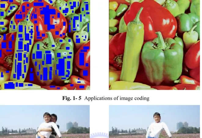
The applications of image inpainting include the restoration of photographs (Fig. 1-1), films and paintings, the removal of objects (Fig. 1-2 to 1-3) and occlusions, such as text, subtitles (Fig. 1-4), stamps and publicity from images, image coding [5] (The objective is to retain only the information which cannot be correctly reconstructed “minute but important details” and to remove as much as possible from the remainder of the image. After data has been transmitted, using inpainting method to reconstruct the image. Fig. 1-5 shows an example. It reduces about 25% data transmission). In addition, inpainting can also be used to produce special effects (Fig. 1-6) and attack against visible watermarking [17].

Because the applications of image inpainting are living, how to effectively and correctly inpaint an unknown region has become an important research issue. In other words, image inpainting has become a paramount research topic in recent year. We are interested in

knowing the well-known inpainting methods. The basic idea is to use undamaged neighboring information to inpaint damaged regions. In section 1.2, we will introduce several well-known inpainting methods and then direct several defects of them. In section 1.3, we will propose a new method that can improve these defects and get better performance.

Fig. 1- 1 Restoration of photographs

Fig. 1- 2 Removal of trees

Fig. 1- 3 Removal of a girl

Fig. 1- 5 Applications of image coding

Fig. 1- 6 Special effects 1.2 Related Works

There are several researches of image inpainting. Bertalmio et al [1] have introduced a technique for digital inpainting of still images that produces very impressive results. Based on partial differential equations (PDEs), the algorithm fills in the damaged areas to be inpainted by propagating information from the outside of the masked region along level lines

(Isophotes).

However, the algorithm usually requires several minutes on current personal computers for the inpainting of relatively small areas. Such a time is unacceptable for interactive sessions and motivated Manuel M. Oliveira, Brian Bowen, Richard McKenna and Yu-Sung Chang [2] to design a simpler and faster algorithm capable of producing similar results in just a few

seconds. It uses a weighted average kernel that only considers contributions from the neighboring pixels. Efficiency of the fast inpainting algorithm is two to three orders of magnitude faster than those using partial differential equations. But it constraints the regions to be inpainted must be locally small. If the damaged regions are not small enough, some possibly important information might be discarded. Results might be blurred.

For inpainting large damaged regions well, Efros and Leung et al. [3] proposed a texture synthesis algorithm to solve the problem. In their algorithm, the lost region is filled-in pixel by pixel with the texture from its neighbors. This algorithm is considerably faster when using the improvements in [10], [18], [19], [20].

Inspired by the work of Efros and Leung [3], Criminisi, Pérez and Toyama proposed an exemplar-based texture synthesis algorithm [7] for removing/inpainting large objects from digital images. Their approach employs an exemplar-based texture synthesis technique modulated by a unified scheme for determining the fill order of the target region. Pixels

maintain a confidence value, which together with image isophotes, influence their fill priority. Viewing from above inpainting techniques, “Fast Digital Image Inpainting” [2] can fast inpaint small damaged regions, but it can’t work well for large damaged regions. “Region Filling and Object Removal by Exemplar-Based Image Inpainting” is also called “Priority Texture Synthesis” [7]. It can both inpaint small and large damaged regions well, but it spend too much time. Therefore, how to correctly and quickly inpaint these images with several small and large damaged regions becomes the goal of our paper.

1.3 Thesis Organization

In this thesis, we propose an image inpainting method that will combine “Fast Digital Image Inpainting” and “Priority Texture Synthesis”. The remainder of this thesis is organized as follows. In chapter 2, we will survey the research of image inpainting and discuss some issues needed to concern. Then, we will describe how to evaluate the similarity value between

two textures. Finally, we will survey the concept of morphological operations. In chapter 3, we will present our method which uses the morphological operator “opening” to split the damaged regions of images into several small and large parts according to the structuring element which users set up. After splitting, we modify the “Fast Digital Image Inpainting” algorithm and apply it to inpaint small damaged parts. Then, we use “Priority Texture Synthesis” to inpaint large damaged parts and add the FFT block matching algorithm to speedup the time of searching similar textures. In chapter 4, we will experiment with different kinds of damaged images. The proposed method can efficiently reduce the cost of

computation. Experimental results look “reasonable” to the human eye. Then, we will

compare the performance of our method with other methods. In chapter 5, the conclusion and future work will be stated.

CHAPTER 2

Previous Research

In this chapter, we will describe several related researches about image inpainting in section 2.1. In section 2.2, we will describe the block matching problem and introduce a faster algorithm for solving it. In section 2.3, the concept of PSNR will be introduced. Basic morphological operators will be described in section 2.4.

2.1 Review of Digital Image Inpainting

The image inpainting methods are widely used in various fields such as wireless communication, reverting deterioration of photographs, image coding (e.g., recovering lost blocks) and special effects (e.g., removal of objects), etc. The basic idea behind the methods that have been proposed in the literature is to fill-in these regions with available information from their surroundings. In this section, we will describe some existed image inpainting algorithms.

2.1.1 Image Inpainting Based on Partial Differential Equation (PDE)

Bertalmio et al [1] pioneered a digital image-inpainting algorithm based on partial differential equations (PDEs). For the damaged image, it fills in the areas to be inpainted by propagating information from the outside of the masked region along level lines (Isophotes). Isophote directions are obtained by computing at each pixel along the inpainting contour a discretized gradient vector (it gives the direction of largest spatial change) and by rotating the resulting vector by 90 degrees (Fig. 2-1 [1]). This intends to propagate information while preserving edges. A 2-D Laplacian [21] is used to locally estimate the variation in color smoothness and such variation is propagated along the isophote direction [1]. After every few

Ω ∈ ∀ + =

∆

+ ) , ( ), , ( ) , ( ) , ( 1 j i j i j i j i

_I

_tI

I

nt n n

step of the inpainting process, the algorithm runs a few diffusion iterations to smooth the inpainted region.

Isophotes

Fig. 2- 1 The figure describes what is Isophote Directions .

Propagation direction as the normal to the signed distance to the boundary of the region to be inpainted.

The algorithm of that form can be written as :

(2.1) where the superindex n denotes the inpainting “time”, (i, j) are the pixel coordinates, ∆t is the rate of improvement and

_I

n_t( ji, ) stands for the update of the image

_I

n( ji, ). Note that

the evolution equation runs only inside Ω, the region to be inpainted.

With this equation, the image

_I

n+1(i,j) is an improved version of

_I

n( ji, ), with the

“improvement” given by

_I

n_t( ji, ). As n increases, we achieve a better image. In section 2.1.1.1, we will introduce how to design the update

_I

n_t( ji, ).

2.1.1.1 How to calculate

_I

n_t( ji, ) ?

) , ( ji

I

nt stands for the update of the image

I

( ji, ) n

. We use partial differential equations to compute it. It can be denoted as :

) , ( ) , ( ) , (i j

_L

n i j

_N

n i j

I

nt ⎯→ ⎯ ⎯→ ⎯ ⋅ =

_δ

(2.2)

where )

δ

_L

n( ji, ⎯→ ⎯

is a measure of the change in the information . With this equation, we estimate the information of our image and compute its change along the

) , ( ji

L

n ) , ( ji

L

n

N

⎯→ ⎯

direction. Note that at steady state, that is, when the equation (2.1) converges,

) , ( ) , ( 1 j i j i

_I

I

n+ = n and from (2.1) and (2.2) we have that (, )⋅ ( , )=0

⎯→ ⎯ ⎯→ ⎯ j i n j i n

N

L

δ

,

meaning exactly that the information L has been propagated in the direction

_N

⎯→ ⎯

. For more details, we now rewrite the equation (2.2) as :

) , ( ) , , ( ) , , ( ) , ( ) , ( i j n j i n j i j i n j i

_I

N

N

L

I

nt

∇

n ⎟ ⎟ ⎟ ⎟ ⎟ ⎠ ⎞ ⎜ ⎜ ⎜ ⎜ ⎜ ⎝ ⎛ ⋅ = ⎯→ ⎯ ⎯→ ⎯ ⎯→ ⎯

δ

(2.3)

On the implementation, we can use discrete equation borrows from the numerical analysis literature. See Section 2.1.1.2, Section 2.1.1.3 and Section 2.1.1.4.

2.1.1.2 How to calculate

δ

_L

n( ji, ) ⎯→ ⎯ ?

(

( 1, ) ( 1, ), (, 1) (, 1)

)

: ) , ( = + − − + − − ⎯→ ⎯ j i j i j i j i j i n

_L

_L

_L

_L

L

n n n n

δ

(2.4) ) , ( ) , ( ) , (i j

_I

i j

_I

i j

L

nyy n xx n + = (2.5) As mentioned above,

δ

_L

n( ji, ) ⎯→ ⎯

is a measure of the change in the information . Let be an image smoothness estimator. For this purpose we may use a

simple discrete implementation of the Laplacian: . Other smoothness estimators might be used, though satisfactory results were already obtained with this very simple selection.

) , ( ji

L

n

_L

n( ji, ) ) , ( ) , ( ) , (i j

_I

i j

_I

i j

L

nyy n xx n + =

2.1.1.3 How to calculate ) , , ( ) , , ( n j i n j i

N

N

⎯→ ⎯ ⎯→ ⎯ ?

(

)

(

(

,

)

) (

2

(

,

)

)

2 ) , ( ), , ( ) , , ( ) , , (

j

i

I

j

i

I

I

I

N

N

n y n x j i j i n j i n j i nx n y + − = ⎯→ ⎯ ⎯→ ⎯ (2.6) ) , , ( ) , , ( n j i n j i

N

N

⎯→ ⎯ ⎯→ ⎯

means the isophote direction. We can compute and

by using some gradient operators (Fig. 2-2)

)

,

( j

i

I

nx

I

ny

( j

i

,

)

-1 1 1 1 0 0 0 -1 -1 -1 1 0 -1 1 0 -1 0 1

I

x

I

y a -1 1 2 1 0 0 0 -2 -1 -1 1 0 -1 2 0 -2 0 1

I

x

I

y b

Fig. 2- 2 Some gradient operators. (a) is Prewitt operator. (b) is Sobel operator.

( )

( ) ( ) ( )

( )

( ) ( ) ( )

, 0, 0 , ) , ( 2 2 2 2 2 2 2 2 ⎪ ⎪ ⎩ ⎪⎪ ⎨ ⎧ < + + + > + + + =

∇

β

β

n n n when n yfm n ybM n xfm n xbM when n yfM n ybm n xfM n xbm j i

I

I

I

I

I

I

I

I

I

(2.7) ) , , ( ) , , ( ) , ( ) , ( n j i n j i j i n j i

N

N

L

n ⎯→ ⎯ ⎯→ ⎯ ⎯→ ⎯ ⋅ =

_δ

β

(2.8) ) , ( ji

I

n

∇

stands for the gradient of the image.

β

n is the projection of

δ

⎯⎯→

_L

onto the normalized vector

_N

⎯→ ⎯

, that is, we compute the change of L along the direction of

_N

⎯→ ⎯

. Finally, we multiply by a slope-limited version of the norm of the gradient of the image. A central differences realization would turn the scheme unstable, and that is the reason for using slope-limiters. The subindexes b and f denote backward and forward differences respectively, while the subindexes m and M denote the minimum or maximum. See [27] for details.

β

n

2.1.2 Fast Digital Image Inpainting

A fast inpainting algorithm was proposed in [2], based on image diffusion kernels. Let Ω be a small area to be inpainted. The simplest version of the algorithm consists of initializing Ω by clearing its color information and repeatedly convolving the region to be inpainted with a diffusion kernel. It uses a weighted average kernel that only considers contributions from the neighboring pixels. Fig. 2-3 [2] shows the pseudocode of the algorithm and two diffusion kernels.

InitializeΩ ;

for (iter =0; iter < num_iteration; iter++) convolve masked regions with kernel;

a b a b 0 b a b a c c c c 0 c c c c

Fig. 2- 3 (top) Pseudocode for the fast inpainting algorithm. (bottom) Two

diffusion kernels used with the algorithm. a= 0.073235, b = 0.176765, c = 0.125.

Efficiency of the fast inpainting algorithm [2] is two to three orders of magnitude faster than those using partial differential equations. But it constraints the regions to be inpainted must be locally small. If the damaged regions are not small enough, some possibly important information might be discarded. Results might be blurred.

We use the fast inpainting algorithm to inpaint the following pictures. Fig. 2-4 and 2-5 are the examples of inpainting locally small damaged regions. The results look good. Fig. 2-6 is the example of inpainting large damaged regions. The result is blurred.

Fig. 2- 5 Lena : (left) Picture with locally small damaged regions. (right) Restored image

obtained with fast inpainting algorithm.

Fig. 2- 6 Lena : (left) Picture with large damaged regions. (right) Restored image obtained

with fast inpainting algorithm.

2.1.3 Texture Synthesis

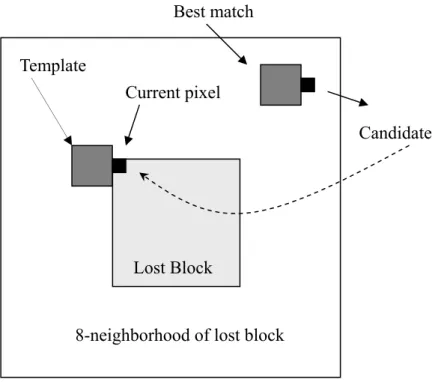
For inpainting large damaged regions well, Efros and Leung et al. [3] proposed an algorithm to solve the problem. In this algorithm, the lost region is filled-in pixel by pixel with the texture from its neighbors. As illustrated in Fig. 2-7 [3], when filling the pixel

, the algorithm first defines a )

, ( ji

p 3×3 template

_I

_t next to p( ji, ), and looks for a

^

I

t

in the available neighboring blocks such that d(

_I

_t,

_I

^_t) is minimized, where ( , )

^

I

I

t t

defined as the normalized sum of squared differences (SSD) metric (More details can be found in section 2.2). Once the nearest template is found, we copy the pixel (candidate) in the correspondent position to our pixel (current pixel) to be filled-in. Fig. 2-8 shows the

algorithm’s results. This algorithm is considerably faster when using the improvements in [10], [18], [19], [20].

Best match

8-neighborhood of lost block

Candidate

Lost Block Template

Current pixel

Fig. 2- 8 Lena : (left) Picture with large damaged regions. (right) Restored image obtained

with texture synthesis algorithm.

2.1.4 Priority Texture Synthesis

Inspired by the work of Efros and Leung, Criminisi, Pérez and Toyama proposed an exemplar-based texture synthesis algorithm [7] for removing large objects from digital images. Their approach employs an exemplar-based texture synthesis technique modulated by a

unified scheme for determining the fill order of the target region. Pixels maintain a confidence value, which together with image isophotes, influence their fill priority. Figure 2-9 [6] shows the pseudocode of the algorithm.

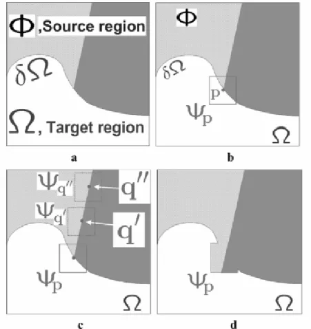
The algorithm

1. Manually select region Ω for removal (Fig. 2-10 a) 2. Repeat until region Ω is empty

1. Compute boundary dΩ and priorities P(p) 2. Propagate texture and structure information

1. Find patch Ψp on dΩ with highest priority P(p) (Fig. 2-10 b) 2. Find patch Ψq in Φ which minimizes SSD(Ψp, Ψq) (Fig. 2-10 c) 3. Copy Ψq to Ψp (Fig. 2-10 d)

3. Update confidence values (More details can be found in section 2.1.4.4)

Fig. 2- 9 The pseudocode of the exemplar-based texture synthesis algorithm.

target region Ω, its contour δ , and the source region Φ clearly marked. (b) We want to Ω

synthesize the area delimited by the patch Ψp centered on the point p∈δΩ. (c) The most likely candidate matches for Ψp lie along the boundary between the two textures in the source region, e.g., and . (d) The best-matching patch in the candidates set has been copied into the position occupied by Ψp, thus achieving partial filling of . Notice that both texture and structure (the separating line) have been propagated inside the target region. The target region has, now, shrunken and its front

Ψ

q'

Ψ

q''

Ω

Ω δ has assumed a different shape. Ω

2.1.4.1 How to calculate P(p)?

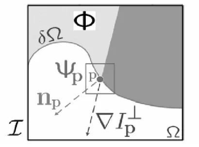
Fig. 2- 11 Notation diagram.

Fig. 2-11 shows the notation diagram [7]. Given a patch Ψq centered at the point p for some p∈dΩ,

n

p is the normal to the contour δ of the target region Ω and is the isophote (direction and intensity) at point p. The entire image is denoted with . We define its priority P(p) as the product of two terms P(p) = C(p) D(p), We call C(p) the

confidence term and D(p) the data term, and they are defined as follows:

Ω ∇

_I

⊥_p

|

|

)

(

)

(

( )

p

q

C

p

C

q p

Ψ

=

∑

∈Ψ ∩ Ι−Ω (2.9)

α

|

|

)

(

I

p

n

p

p

D

=

∇

⋅

⊥ (2.10) where is |Ψp | the area of Ψp, α is a normalization factor (e.g., α = 255 for a typical grey-level image), (More details can be found in section 2.1.4.2) is a unit vector orthogonal to the front dΩ in the point p, and

p

n

⊥ (More details can be found in section

2.1.4.3) denotes the orthogonal operator. The priority P(p) is computed for every border patch, with distinct patches for each pixel on the boundary of the target region. During initialization, the function C(p) is set to C(p) = 0 ∀p∈Ω and C(p) = 1 ∀p∈Ι−Ω.

2.1.4.2 How to calculate

n

p ?

Given a point p∈dΩ, the normal direction is computed as follows : 1) the positions of the “control” points of dΩ are filtered via a bidimensional Gaussian kernel (Fig. 2-12) and, 2) is estimated as the unit vector orthogonal to the line through the preceding and the successive points in the list. Alternative implementation may make use of curve model fitting [23]. p

n

p

n

0 0 0 -1 0 0 2 0 -1 0 0 0 0 -1 2 -1 0 0 Gy Gx

Fig. 2- 12 A bidimensional Gaussion Kernel filter

I

p

⊥

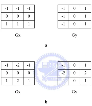
∇ denotes the orthogonal gradient vector. The gradient is computed as the maximum value of the image gradient in

I

p ∇

Ι ∩

Ψp . Robust filtering techniques may also be employed here, such as using some gradient operators (Fig. 2-13). After computing ,

(-Gy, Gx) is the orthogonal gradient vector .

I

p ∇

I

p ⊥ ∇ -1 1 1 1 0 0 0 -1 -1 -1 1 -1 0 1 -1 0 0 1 Gx Gy a -1 1 2 1 0 0 0 -2 -1 -1 1 -1 0 2 -2 0 0 1 Gx Gy b

Fig. 2- 13 Some gradient operators. (a) is Prewitt operator. (b) is Sobel operator.

2.1.4.4 How to update confidence value ?

After the patch has been filled with new pixel values, the confidence C(p) is

updated in the area delimited by

Ψ

^ p

Ψ

^ p, as follows: Ω ∩ Ψ ∈ ∀ = ₍∧_), ^ ) (p C p p _p C (2.11)

front without image-specific parameters. As filling proceeds, confidence values decay, indicating that we are less sure of the color values of pixels near the center of the target region.

2.2 Block Matching

The block matching problem is one that occurs in various fields of applications, such as the image processing, multimedia and vision fields. The basic idea for solving the block matching problem is to minimize some measure of similarity between a template block of pixels in the current image to all candidate blocks in the reference image within a given search range. In this section, we will describe a new algorithm [10] for solving the block matching problem which is independent of image content and is faster than other full-search methods.

2.2.1 SAD and SSD

We first introduce two most popular similarity measures. They are defined as :

∑∑

− = − = − + + − = 1 0 1 0 1 ) , ( (, ) ( , ) B j B i t t v u

f

i j

f

i u j v

SAD

(2.12)

(

)

∑∑

−

−

+

+

= − = − = 1 0 1 0 2 ) , (

(

,

)

1

(

,

)

B j B i v u

f

i

j

f

i

u

j

v

SSD

t t (2.13)

SAD means the sum of absolute difference and SSD means the sum of squared difference. B is a block size and (u, v) is a displacement vector for a candidate block relative to the template block. Lets compare the difference between SAD (2.12) and SSD (2.13). Because of its lack of multiplications, the SAD metric is far more convenient for use in hardware designs, and is therefore used almost exclusively. However, minimizing the SSD metric corresponds to maximizing the PSNR (More details can be found in section 2.3). If a maximum PSNR is desired, SSD should be the metric of choice. Therefore, we choose SSD metric to measure

2.2.2 The FFT Block Matching Algorithm

Steven L. Kilthau, Mark S. Drew, and Torsten Möller et al. [10] proposed an FFT Block matching algorithm. It is faster than other full-search methods. In order to maximize the PSNR, the algorithm minimizes the SSD metric given in Eq.2.13. Following a trivial expansion, the mathematical definition of the per-block computation is given by:

[

]

(2.14) 1 1 2 2 1 0 1 0 ,

(

,

)

(

,

)

2

(

,

)

(

,

)

min ∑∑

−

+

+

+

−

+

+

= − = ∀ _{− −} B j B i v u

f

i

j

f

i

u

j

v

f

i

j

f

i

u

j

v

t t t t

Since the term appears across the entire minimum, it can be removed from the sum without affecting the resulting solution. Removing this term and separating the sum leaves us with the following equation:

2

)

,

( j

i

f

_t

∑∑

∑∑

+

+

− = − = − − = − = ∀ − − + + 1 0 1 0 1 1 0 1 0 2 , 1

(

,

)

2 ( , ) ( , )

min

B j B i t t B j B i v u

f

_t

i

u

j

v

f

i j

f

i u j v (2.15)

Finally, we employ a novel data structure called the Windowed-Sum-Squared-Table and use the fast Fourier transform (FFT) in its computation of the sum squared difference (SSD) metric. Figure 2-14 shows the three basic steps of the FFT Block Matching algorithm.

The Algorithm

1. Resize input image to include a zero pad (More details can be found in section 2.2.2.1) 2. Compute the windowed sum squared table

(More details can be found in section 2.2.2.2) 3. Compute a per-block convolution sum

(More details can be found in section 2.2.2.3)

Fig. 2- 14 FFT Block Matching algorithm.

∑ ≤ ∑ ≤

=

_{k i} l j

SAT

i

j

f

k

l

f

(

,

)

(

,

)

Given a search range of ±P we apply a zero pad of P pixels around the entire image. This simple preprocess eliminates the need for conditionals within the innermost loops of our algorithm and greatly increases its speed. In other words, it is simply to allow convenient calculation of the SSD metric without using conditionals for those search locations that lie outside of the dimensions of the original image.

2.2.2.2 Windowed Sum Squared Table

We use a variant of the well known summed area table (SAT), introduced in [24]. Given an input image f , a summed area table is a new image

_f

such that

SAT

(2.16) Summed area tables can be very easily computed by applying the following recurrence, being careful to set

f

( j

i

,

)

to zero when either of the indices is negative:

[

(

,

)

(

1

,

)

(

,

1

)

(

1

,

1

)

]

)

,

(

i

j

=

f

i

j

+

f

i

−

j

+

f

i

j

−

−

f

i

−

j

−

f

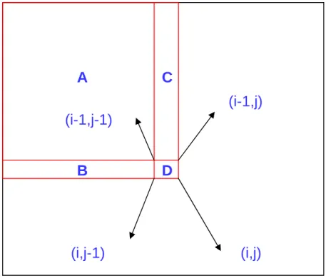
_{SAT SAT SAT SAT} (2.17)

Fig. 2- 15 A simple example for computing SAT. C B A D A B A C A j i f SAT i j f (, )= (, )+( + )+( + )− = + + +

The WSST differs from the SAT in that each pixel needs to represent a sum of squares, where the sum extends only over the last B × B sub-image (window), with B the block size.

[

(

,

)

(

1

,

)

(

,

1

)

(

1

,

1

)

]

)

,

(

i

j

=

f

i

j

2

+

f

i

−

j

+

f

i

j

−

−

f

i

−

j

−

f

_{SST SST SST SST} (2.18)

[

] [

] [

[

(

1

,

1

)

(

,

)

(

,

1

)

(

1

,

)

]

(

2

.

19

)

)

,

(

)

1

,

(

)

,

(

)

,

1

(

)

,

(

)

,

(

)

,

(

2 1 1

B

j

f

B

i

f

B

j

B

i

f

f

B

j

i

f

i

f

j

B

i

f

j

f

j

i

f

t

s

f

j

i

f

SST SST SST SST SST SST SST SST SST i B i t j B j s WSST

−

−

−

−

−

−

−

−

+

−

−

+

−

−

−

+

−

−

−

+

=

=

∑ + − = ∑ + − =

]

2.2.2.3 Per-Block Convolution Sum

We show that computation of the second term in Eq.2.15 amounts to the evaluation of a correlation sum for each template block, which we evaluate as a convolution sum.

∑∑

− = − = − + + 1 0 1 0 1 ) , ( ) , ( B j B i t t v j u i j i

f

f

(2.20)

A

C

(i-1,j)

(i-1,j-1)

B

D

(i,j)

(i,j-1)

(

)

∑∑

− = − = − − + + = = • 1 0 1 0 1 1( , ) ( ) ( ) ) , ( B j B i t t candidates FFT template FFT FFT result v j u i j i

f

f

In order to efficiently compute the correlation, we will convert it to a convolution (Eq.2.20) and then use the Fast Fourier transform. For each template block, we create two images of size (2P+B)*(2P+B). The first image, template , corresponds to the template block and is computed by simply multiplying the block by 2, reversing the pixels, and zero padding to the correct size. The pixel reversal effectively changes the correlation sum into an equivalent convolution sum. The second image, candidates , corresponds to the square containing all pixels of all candidate blocks in the search range. This square can be copied directly from the reference image. Given these two images, we can compute a new image, result , according to the following formula:

(2.21)

2.3 PSNR

Signal-to-noise (SNR) measures are estimates of the quality of reconstructed images compared with their original images. The basic idea is to compute a single number that reflects the quality of a reconstructed image. Reconstructed images with higher metrics are judged better. The actual metric we will compute is the peak-signal-to-reconstructed image measure which is called PSNR. The higher measures might mean better quality. Assume we are given a source image f(i,j) that contains N by N pixels and a reconstructed image F(i,j) which is reconstructed by inpainting a damaged version of f(i,j). The pixel values f(i,j) range between black (0) and white (255). We compute the mean squared error (MSE) of the

reconstructed image as follows :

[

]

2 2

)

,

(

)

,

(

N

j

i

F

j

i

f

MSE

=

∑

−

_(2.22)

The root mean squared error (RMSE) is the square root of MSE :

[

f

i

j

−

F

i

j

]

∑

2

)

,

(

)

,

(

PSNR in decibels (dB) is computed as follows:

)

255

log(

10

2

MSE

PSNR

=

_(2.24) 2.4 Mathematical Morphology

Mathematical morphology is a tool for extracting image components that are useful in the representation and description of region shapes, such as boundaries, skeletons, and convex hulls. Mathematical morphology is a set-theoretic method. Sets in mathematical morphology represent the shapes of objects in an image. The operations of mathematical morphology were originally defined as set operations and shown to be useful for image processing.

In general, morphological approach is based upon binary images. In binary images, each pixel can be viewed as an element in 2

Z . Gray-scale digital images can be represented

as sets whose components are in 3

Z , two components are the coordinates of a pixel, and the

third corresponds to its discrete intensity value. The morphological operations input a source image and a structuring element which is another image usually smaller than the source image. The structuring element is a predetermined geometric shape, and there are some common structuring elements as shown in Fig. 2-16.

1 1 1 1 1 1 1 1 1 1 1 1 1 1 1 1 1 1 1 1 1 1 1 1 1 1 1 1 1 1 1 1 1 1 1 1 1 1 1 1 1 1 1 1 1 1 1 1 1 1 1 1

Fig. 2- 16 Examples of structuring elements

Here, we will discuss morphological operators in binary images [25, 26]. Given a source image A and a structuring element B in 2

2.4.1 Basic definition

The Translation of A by the point x in 2

Z , denoted A_xv, is defined by

{

|

}

x

Av = av v+x ∀ ∈av A = +A xv (2.25) where the plus sign refers to vector addition.

And the Reflection of B, denoted Bˆ , is defined as

{

|

}

B= −b bv v∈B (2.26) The examples of Translation and Reflection are shown in Fig. 2-17.

xv A B x Av (a) (b) Bˆ

Fig. 2- 17 Examples of (a) Translation and (b) Reflection

2.4.2 Morphological operations

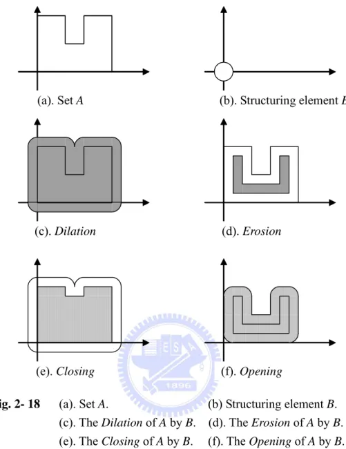
Here, we introduced two of the fundamental morphology operations：Dilation and Erosion used in binary images, and introduced two operators：Closing and opening that extended from Dilation and Erosion.

2.4.2.1 Dilation and Erosion

The Dilation of A by B, denoted D_B

( )

A , is defined as

( )

ˆ

{

_| ˆ

}

B

D A = ⊕ =A B x Bv + ∩ ≠xv A φ (2.27)

Where B is the structuring element.

The examples of Dilation and Erosion are shown in Fig. 2-18 (c) and (d). The dilation of A by

B is the set of all xv displacements such that Bˆ and A overlap by at least one nonzero

element. The erosion of A by B is the set of all points xv such that B translated by xv is contained in A.

2.4.2.2 Closing and Opening

The Closing of set A by structuring element B, denoted CB

( )

A , is defined as

( )

ˆ

(

( )

)

(

ˆ

)

ˆ

B _B B

C A = • =A B E D A = A⊕ 0B B (2.29)

And the Opening of set A by structuring element B, denoted O_B

( )

A , is defined as

( )

ˆ

(

( )

)

(

)

B B

O A = A B_o =D_B E A = A B0 ⊕B (2.30)

The examples of Closing and Opening are shown in Fig. 2-18 (e) and (f). The closing of A by

B is simply the dilation of A by B, followed by the erosion of the result by Bˆ . The opening of A by B is simply the erosion of A by B, followed by the dilation of the result by Bˆ .

(a). Set A (b). Structuring element B

(c). Dilation (d). Erosion

(e). Closing (f). Opening

Fig. 2- 18 (a). Set A. (b) Structuring element B.

(c). The Dilation of A by B. (d). The Erosion of A by B.

(e). The Closing of A by B. (f). The Opening of A by B.

2.4.3 Extension to Gray-Scale Images

In this section we extend to gray-level images the basic operations of dilation, and erosion. Throughout the discussions that follow, we deal with digital image functions of the forms f x y and( , ) b x y( , ), where f x y is the gray-scale image and( , ) is a structuring

element.

( , )

b x y

Gray-Scale dilation of f by , denoted by b f ⊕ , is define as：b

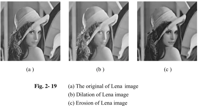
element of the morphological process but note that b is now a function rather than a set. Because dilation is based on choosing the maximum value of f + b in a neighborhood defined by the shape of the structuring element, the general effect of performing dilation on a gray-scale image is two-fold: (1) if all the values of the structuring element are positive, the output image tends to be brighter than the input; and (2) dark details either are reduced or eliminated, depending on how their values and shapes relate to the structuring element used for dilation. As illustrated in Fig 2-19 (b).

Gray-scale erosion of f by , denoted by b f0 , is define as： b

(f0b s t)( , ) min{ (= f s+x t, +y)−b x y( , ) (s+x), (t+y)∈D_f;( , )x y ∈D_b}

b

D

(2.32)

Where D_f and are the domain of f and b . Because erosion is based on choosing the

minimum values of f b− in a neighborhood defined by the shape of the structuring element, the general effect of performing erosion on a gray-scale image is two-fold: (1) if all the values of the structuring element are positive, the output image tends to be darker than the input; and (2) bright details are reduced or eliminated, depending on the used structuring element. As illustrated in Fig 2-19 (c).

(a ) (b ) (c )

Fig. 2- 19 (a) The original of Lena image

(b) Dilation of Lena image (c) Erosion of Lena image

The usage of closing and closing is to smooth contours of objects. In gray-level images, closing is used for brighter objects with darker background, and opening is used for darker object objects with brighter background. As illustrated in Fig 2-20 (b) and (c).

(a ) (b ) (c )

Fig. 2- 20 (a) The original of Lena image

(b) Closing of Lena image

(c) Opening of Lena image

2.4.4 Morphological Gradient

The Morphological Gradient of an image, denoted G:

( )

( ) (

) (

)

B B G=D A −E A = A⊕B − 0A B (2.33) or

( )

(

)

(2.34) B G=D A − =A A⊕B −A or

( )

(

)

(2.35) B G= −A E A = − 0A A B

The morphological gradient highlights sharp gray-scale transitions in the source image. In other words, morphological gradient can extract the boundary of an object. However, the morphological gradient is sensitive to the shape of the chosen structuring element. Here are examples of dilation, erosion, closing, opening, and morphological gradient of the gray-scale

image, Lena, with the 3×3 structuring element as shown in Fig 2-21.

(a ) (b )

Fig. 2- 21 (a) The original of Lena image

CHAPTER 3

The Proposed Method

In this chapter, we will introduce the architecture of the inpainting system based on the proposed method. We focus on these images with several small and large damaged regions, such as the image shown in Fig. 3-1. The goal of this paper is to effectively and correctly inpaint these damaged images. It is known that “Fast Digital Image Inpainting” [2] can fast inpaint small damaged regions, but it can’t work well for large damaged regions. “Priority Texture Synthesis” [7] can both inpaint small and large damaged regions well, but it spend too much time. Therefore, we propose a new inpainting method that will combine “Fast Digital Image Inpainting” and “Priority Texture Synthesis”. In section 3.1, we will discuss the process of our image inpainting. In section 3.2, we will utilize morphological operations to

automatically split the damaged regions into several small and large parts. In section 3.3, we will modify the “Fast Digital Image Inpainting” algorithm and then apply it to inpaint these small damaged parts. In section 3.4, we will apply the “Priority Texture Synthesis” algorithm to inpaint these large damaged parts and add the FFT block matching algorithm to speedup the time of searching similar textures. Finally, we will summarize the proposed method in Section 3.5.

3.1 Overview of Our Image Inpainting System

We designed a simple drawing interface, which allows users to draw lines or surfaces. Users need to input a damaged image at the start of the inpainting process. As illustrated in Fig. 3-2, when users mark these damaged regions from the input image, the system will split the damaged regions into several small and large parts according to the structuring element

splitting result, we can re-set up the structuring element to split the damaged regions. After splitting these damaged regions, the system will automatically use “Fast Digital Image Inpainting” to inpaint small damaged parts and use “Priority Texture Synthesis” to inpaint large damaged parts. At last, the system will not only show the reconstructed result but also show several intermediate steps of the reconstruction on the interface.

Opening

Mark Damaged Regions

Small Damaged Regions Large Damaged Regions

Priority Texture Synthesis Fast Digital Image Inpainting

Original Image

Output Image

3.2 Splitting the damaged regions into several small and large parts

Morphologigical operators are attractive because they involve simple logical operations and can be easily implemented. A fundamental feature of mathematical morphology is the use of a structuring element. This is essentially a smaller version of the input image, and contains structure of the type that is to be analyzed in the image. The two basic morphological

operators are dilation and erosion. Dilation expands (for binary image) and brightens (for gray-scale image) an image, while erosion shrinks and darkens. Dilation is performed by sliding the structuring element over the image while adding the values of the structuring element to the image, and then recording the maximum value reached at each point. Erosion is similar, except that the structuring element values are subtracted from the image, and the global minimum is taken.

The opening operation is created by first eroding and then dilating an image. Physically, the binary opening operation extracts some shapes whose sizes are larger enough than the structuring element. As illustrated in Fig. 3-3, there are some shapes numbered from 1 to 6. After opening, we see that this operation extracts shape 5, 6 and discards shape 1, 2, 3, 4. Fig. 3-4 is an opening operation example for a binary image. It extracts the shapes whose sizes are larger than 9*9 window size according to 9*9 structuring element.

Viewing from another angle, we can apply the opening operation to split the damaged regions into several small and large parts according to the structure element for our test images. There are two examples. Fig. 3-5 (b) splits the damaged regions into two parts by using “opening” according to 3*3 structuring element. “Green” represents small damaged parts and “Blue” represents large damaged parts. Similarly, Fig. 3-6 (b) splits the damaged regions into two parts by using “opening” according to 3*3 structuring element. “Yellow” represents small damaged parts and “Blue” represents large damaged parts.

Fig. 3- 3 (a) Set A (b) Structuring element B (c) The Opening of A by B.

Fig. 3- 4 (a) A binary image : A (b) The Opening of A by 9*9 structuring element.

5 2 3 1 4 6 (a) (b) (c) (a) (b)

(a) (b)

Fig. 3- 5 (a) A damaged elliptic image (b) Splits the damaged regions into two parts

(a) (b)

Fig. 3- 6 (a) A damaged lena image (b) Splits the damaged regions into two parts

3.3 Using “Fast Digital Image Inpainting” to inpaint these small damaged parts

The fast inpainting algorithm can faster inpaint the locally small damaged regions well than other methods. Here, we modify the “Fast Digital Image Inpainting” algorithm and let it be more performance. The new algorithm doesn’t setup iterative-times. We will apply it to inpaint these small damaged parts after splitting. The modification of this algorithm is described as below：

The new algorithm

1. After splitting, the algorithm automatically selects these small damaged regions Ω . 2. Repeat until region Ω is empty

2.1. Mark boundary dΩ.

2.2. For each boundary pixel, compute the average of its undamaged neighborhood pixels, and then copy it to the boundary pixel. 2.3. Update these small damaged regions Ω

Fig. 3- 7 The pseudocode of the algorithm

M M M M M D D D M D M M M M M M M M M M M M M D D DD D D D D D D D D D D D D D D D D D D D (a) (b) I I I I I D D D I D I I I I I I I I I I I I I I I I I I M M M I M I I I I I I I I I I I I I (c) (d)

I I I I I I I I I I I I I I I I I I I I I I I (e)

Fig. 3- 8 The step by step example shows how the algorithm inpaints these small

damaged regions.

Let us see an example. As illustrated in Fig. 3-8, the algorithm first selects these small damaged regions Ω “Red D” (Fig. 3-8. a). Because Ω is not empty, the algorithm marks the boundary “Blue M” (Fig. 3-8. b). For each “Blue M”, compute the average of its undamaged neighboring pixels, and then copy it to the boundary pixel. “Green I” represents the region which has been inpainted (Fig. 3-8. c). The algorithm updates the damaged regions

, and then repeats previous steps untill

Ω

d

Ω Ω is empty (Fig. 3-8. d and 3-8. e). Our test

images are shown in Fig. 3-9 and 3-10.

Fig. 3- 9 (a) A Splitted elliptic image (b) The small damaged parts “Green” has been

inpainted well by this algorithm.

(a) (b)

Fig. 3- 10 (a) A Splitted lena image (b) The small damaged parts “Yellow” has been

inpainted well by this algorithm.

3.4 Using “Priority Texture Synthesis” to inpaint these large damaged parts

After inpainting these small damaged regions, there only remains the larged damaged regions. The “priority texture synthesis” algorithm can efficiently and correctly inpaint the large damaged regions. Therefore, we will apply it to inpaint these large damaged parts. At the same time, we will also add the FFT block matching algorithm from section 2.2.2 to speedup the time of searching similar textures. Our test images are shown in Fig. 3-11 and 3-12.

Fig. 3- 11 (a) An elliptic image followed by Fig. 3-9. b (b) The large damaged parts

“Blue” has been inpainted well by priority texture synthesis.

(a) (b)

Fig. 3- 12 (a) A lena image followed by Fig. 3-10. b (b) The large damaged parts “Blue”

has been inpainted well by priority texture synthesis.

3.5 Summation

The proposed method combines “Fast Digital Image Inpainting” and “Priority Texture Synthesis” to inpaint the damaged images. The procedure first uses “opening” to split the damaged regions into several small and large parts. After splitting, it will automatically use “Fast Digital Image Inpainting” to inpaint small damaged parts and use “Priority Texture Synthesis” to inpaint large damaged parts. Experimental results indicate that our method can not only inpaint these damaged images well but also efficiently save computational time. More experimental results and comparisons are shown in Chpater 4.

CHAPTER 4

Experimental Results

In this chapter, we will present more experimental results and comparisons obtained by applying the proposed method described in chapter 3. In section 4.1, we will introduce our experiment environment. Experimental results and comparisons are shown in section 4.2.

4.1 Experimental Environment

In this section, we will first use a simple drawing interface to draw lines or surfaces in the images of every class. We damage edges as seriously as possible and then produce these damaged images which are shown in Fig. 4-1. Based on these same damaged images from classes a to f, we will compare the proposed method with pure fast digital image inpainting [2] and pure priority texture synthesis [7]. Based on these images from classes g to i, we will use the proposed method to remove some objects. The proposed method has been implemented on PC with Pentium4 1.8G, RAM 1024 Megabytes. The operating system is Microsoft Windows XP Server Chinese version Service Pack2. The program was developed in the C++ language and compiled under Borland C++ Builder version 6.0.

Original image Original image Original image

Damaged image

Class a. Elliptic image

Damaged image

Class b. “Lena” image

Damaged image

Class c. “Baboon” image

Original image Original image Original image

Damaged image

Class d. “Pepper” image

Damaged image

Class e. “F16” image

Damaged image

Original image Original image Original image

Damaged image

Class g. Tree image

Damaged image

Class h. Fishing Boat image

Damaged image

Class i. Girl image Fig. 4- 1 There are some test images. Top images of every class are original images.

Bottom images of every class are damaged images.

4.2 Experimental Results

4.2.1 Comparison of inpainting results

Here, we apply the proposed method to a variety of images. Where possible, we make side-by-side comparisons to two other methods from Fig. 4-2 to 4-11.

Fig. 4-2 (a) is the result of Fast Digital Image Inpainting. It spends 0.032 seconds on inpainting. The central damaged rectangle can’t be inpainted well. Elliptic Edges are blurred; Fig. 4-2 (b) shows its intermediate inpainting steps. (Top-left represents 0% inpainting result. It also means the original damaged image. Top-center and Top-right individually represent 20% and 40 % inpainting result. Bottom-left, Bottom-center and Bottom-right individually represent 60%, 80% and 100 % inpainting result.). Fig. 4-3 (a) is the result of Priority Texture