國
立
交
通
大
學
多媒體工程研究所
碩
士
論
文
利用前額訊號偵測駕駛者
在虛擬駕車環境中的清醒程度
Using Forehead-Channel Activities to Detect Driver’s
Drowsiness in a VR Based Driving Environment
研 究 生:陳柏銓
指導教授:林進燈 教授
利用前額訊號偵測駕駛者在虛擬駕車環境中的清醒程度
Using Forehead-Channel Activities to Detect Driver’s Drowsiness in a VR Based Driving Environment
研 究 生:陳柏銓 Student:Po Chuan Chen
指導教授:林進燈 Advisor:Dr. Chin Teng Lin
國 立 交 通 大 學
多 媒 體 工 程 研 究 所
碩 士 論 文
A Thesis
Submitted to Institute of MultimediaEngineering College of Computer Science
National Chiao Tung University in partial Fulfillment of the Requirements
for the Degree of Master
in
Computer Science July 2008
Hsinchu, Taiwan, Republic of China
利用前額訊號偵測駕駛者在虛擬駕車環境中的清醒程
度
研究生:陳 柏 銓
指導教授:林 進 燈 教授
國立交通大學多媒體工程研究所
Abstract in Chinese
摘 要
根據過去研究顯示,跟人類打瞌睡有很強的關聯性的腦區主要是跟枕葉區的 腦波變化(8~12Hz)有很高的相關。然而,若要在真實生活中要使用傳統的電極帽 來擷取腦電波訊號是相當不方便的,而且需要繁複的準備流程,對駕駛者也相當 困擾。因此本論文的主要目的就是要使用前額的電極來偵測駕駛者的精神狀態並 且預測開車軌跡,這樣一來我們就能在真實的生活當中建立一個較為可行的偵測 系統。 本論文主要分析並且比較了分別來自於枕葉區還有額葉區的腦波訊號。而 來自於這些區域的頻率能量變化將會被用來當作輸入參數並且使用線性回歸模 型來預測駕駛者的開車軌跡。而根據我們的結果,使用來自枕葉區的訊號可以得 到最高的預測率。 此外,我們也證明了有一個跟打瞌睡相關的腦區位於額葉區,結果顯示4~ 7Hz頻帶的變化跟打瞌睡有很高的相關性。而使用前額電極的訊號來預測開車軌 跡,雖然比使用枕葉區的準確率來的差一些但仍有八成的準確率,但這意味著使 用前額電極的訊號就可以預測駕駛者的精神狀態,如此一來就可以省下使用電極 帽而帶來的複雜準備程序,這樣的偵測系統在未來就可以被廣泛且容易的被使用 在真實的駕車環境當中。 關鍵字:瞌睡偵測,腦電波,前額電極,虛擬實境,線性回歸,獨立成分分析。Using Forehead-Channel Activities to Detect Driver’s
Drowsiness in a VR Based Driving Environment
Student: Po-Chuan Chen
Advisor: Prof. Chin-Teng Lin
Institute of Multimedia Engineering
National Chiao Tung University
Abstract in English
Abstract
Previous studies showed that the alpha power increases in the occipital lobe highly related to human drowsiness. However, the acquisition of occipital EEG signals with the traditional electrode cap is inconvenient. Thus, the main purpose of this study was to confirm whether the forehead EEG signals could reflect the driver’s drowsiness and be able to use to estimate driver’s driving trajectory for constructing a feasible detecting system that can be applied in real life.
Brain signals acquired from the occipital and the frontal lobe were analyzed and compared in this study. The frequency power changes in these components were used as features and fed into linear regression model to predict driver’s driving performance. Results showed the highest estimation accuracy was yielded with the features extracted from the occipital ICs cluster.
We also found that there is another drowsiness-related brain source located in the frontal lobe. Furthermore, the increases of the theta power in the frontal lobe also highly correlated to the driver’s drowsiness. Comparing the conventional methods using the occipital activities, the estimation accuracy using the forehead signals is slightly lower but the estimation accuracy was still higher than 0.8.
Results demonstrated that forehead signals could be used to estimate the drivers’ drowsiness. The new detecting system, using forehead signals, not only can correctly estimate the user’s drowsiness but also can drastically reduce the preparation time. In the future, such detection system will be easily and widely applied in the real operational environments.
Keywords: Drowsiness, Electroencephalogram (EEG), Forehead Channel, Virtual
誌 謝
Acknowledgement 本論文的完成,首先要感謝我的指導教授 林進燈博士在過去兩年研究期 間,提供豐富的研究資源和實驗環境,並從旁指導協助,使得本文得以順利完成。 其次,我要感謝我的父母對我的照顧與栽培,教導我做人品德為最,強調人 格健全之發展與學習生活之態度,由於他們辛勞的付出和細心的照顧,才有今天 的我。 特別感謝美國加州聖地牙哥大學的 鐘子平教授、 段正仁教授,給予我研究 上最大的協助,從實驗設計、實驗分析、實驗結果討論到論文撰寫,給我最專業 的意見跟看法。 另外,我要感謝腦科學研究實驗室的全體成員,沒有他們也就沒有我個人的 成就。特別感謝 梁勝富教授、 曲在雯博士給予我在各方面的指導,無論是研究 上疑難的解答、研究方法、寫作方式、經驗分享等惠我良多。另外要感謝玠瑤、 尚文、德正、青甫、依伶、孟修、君玲同學,在過去兩年研究生活中同甘共苦, 相互扶持。此外,我也要感謝陳玉潔學姊、柯立偉學長、黃騰毅學長與趙志峰學 長在研究上的幫助,還有感謝建安、馥戍、華山、昂穎、俞凱以及睿昕學弟妹, 在過去這一年中的相伴,以及碩士班新生謹譽、佳鈴在過去一個多月的協助。同 樣地也感謝實驗室助理Amy, Ivy, May, Jenny, Vicky, Kate, Jessica, Nao, Frank,紹 瑋在許多事務上的幫忙以及陪伴。謹以本文獻給我親愛的家人與親友們,以及關心我的師長,願你們共享這份 榮耀與喜悅。
Content
Abstract in English...2
Abstract in Chinese...1
1.
Introduction ...6
1.1 Importance of the drowsiness detecting... 6
1.2 Drowsiness measurements... 6
1.2.1 Signal-based drowsiness system... 7
1.2.2 A Better EEG Measure Technology... 7
1.3 The frontal signals... 8
1.4 The aims of this study ... 9
2.
Materials and Methods...10
2.1 Virtual-reality-based highway driving simulator ... 10
2.2 Subjects ... 10
2.3 The lane keeping driving task... 11
2.4 EEG data acquisition ... 12
2.5 Behavioral data analysis... 12
2.6 EEG data analyses ... 13
2.6.1 EEG Data pre-processing ... 13
2.6.2 Independent Component Analysis... 14
2.6.3 Dipole source localization... 15
2.6.4 Moving-averaged power spectra analysis ... 15
2.6.5 Correlation analysis ... 16
2.6.6 Feature extraction and drowsiness estimation ... 16
2.6.7 LDE sorted spectral analysis... 17
3.
Results ...18
3.1 OM and FCM ICs clusters ... 18
3.2 Coherence between FCM and OM component ... 20
3.3 Relationship between FCM Component and Forehead Component ... 20
3.4 LDE Estimation... 21
3.5 LDE sorted spectral analysis of ICA components... 23
4.
Discussion ...24
4.1 Drowsiness detection... 24
4.2 Coupling between FCM and OM ICs clusters. ... 25
4.3 EEG phenomenon comparing to other studies... 25
4.4 Selecting several forehead channels comparison ... 26
5.
Conclusions...27
Figure List
Fig. 2-1: Pictures show the dynamic virtual reality (VR) driving environment. … 34
Fig. 2-2: The four-lanes road of the VR scene. ……… 35
Fig. 2-3: A bird’s eye view of the lane keeping driving event. ……….35
Fig. 2-4: The analysis of driving trajectories ……….36
Fig. 2-5: Pictures shows the placement and the positions of the forehead 15-channel……….37
Fig. 2-6: The flowchart of the EEG signal analysis. ………37
Fig. 2-7: The identified artifacts. ……….38
Fig. 2-8: The flowchart of the Independent component analysis (ICA). ………….39
Fig. 2-9: The scalp topographies of ICA weighting matrix W. ……….40
Fig. 2-10: The flowchart of the time-frequency analysis. ……….41
Fig. 2-11: An example of linear regression estimation ……….41
Fig. 2-12: The LDE sorted spectrum analysis. ……….42
Fig. 3-1: Equivalent dipole source location, spectra, and the scalp maps …………43
Fig. 3-2: Equivalent dipole source location, spectra, and the scalp maps …………44
Fig 3-3: The coherence between the frontal and the occipital component …………45
Fig. 3-4. The grand means of the frontal component and the forehead component. ..45
Fig 3-5: The grand mean and the standard error of the LDE sorted theta and alpha band power ……….46
Table List
Table 1: The summary of driving performance estimation ……….46Table 2: The comparison of driving performance estimation using forehead channel ………48
1. Introduction
1.1
Importance of the drowsiness detecting
Driving has become one of the most indispensable cognitive behaviors in our daily life. Such a cognitive performance highly involves attention, decision making, information perception and awareness, and coordination of sensorimotor systems. Therefore, decrease in driver’s attention or, more precisely, vigilance level may deteriorate driver’s driving performance and potentially cause car accidents. National Highway Traffic Safety Administration (NHTSA) in the US reported at least 100,000 car crashes were caused by drivers’ falling asleep [4]. Other studies also pointed out that fatigue, which, in turn, caused drowsiness or falling asleep, was one of the major causes of car accidents [1]-[3]. Such dramatic amount of tragic events caused by drivers’ drowsiness call for the attention and demand in devising an online, real-time drowsiness detection and monitoring system to assist and warn drivers when they become drowsy, such that we can best reduce the car accidents caused by drivers’ decreasing driving performance due to drowsiness.
1.2
Drowsiness measurements
In previous studies, drivers’ drowsiness states were mostly derived from different physiological measures based on either signal- or image-based technique. The image-based technique employs video camera to detect, such as, eyelid closure, eyes’ gaze positions, head movements, etc., and derive, for example, the consecutive time periods of eyes closing, duration of gaze fixation, or alike, from such measures
to correlate with drivers’ drowsiness levels [7]-[13]. Such image-based technique requires nearly no preparation, in terms of applying electrodes or sensors, to drivers. However, image-based methods may suffer from the environments with which the video cameras need to interact. For example, in the limited space of driving cabin, it is difficult to find a place to mount two video cameras, in the same time, without blocking the perception of the video cams by the handling wheel.
1.2.1
Signal-based drowsiness system
Most signal-based drowsiness monitoring systems use electrocardiograph (ECG), electroencephalograph (EEG) [17]-[22], or electrooculograph (EOG) [15][16] to monitor drivers’ physiological changes related to their drowsiness levels. However, among these physiological changes, heart rate variability (HRV) [14] derived from ECG measures can be altered by all sorts of physiological or cognitive states and lack of specificity as an index of drowsiness levels. On the other hand, although EOG was used to index the decline of saccade frequency and velocity, which was proved highly related to the driving performance, it suffered from long average windows to establish the evidence for drowsiness and could not be used as a real-time warning system. Other method, such as monitoring the patterns of drivers’ moving handle wheel as used by Toyota Motor Company[5][6], may also highly depend on drivers’ driving behaviors and experience, road conditions, and all other environmental variables, and thus is difficult to be generalized for regular use. As a result, EEG remains the most popular modality used to monitor drowsiness state in real-time.
The power changes in EEG alpha (8-12 Hz) and theta (4-7 Hz) bands have been widely used to index the alertness levels of human subjects in other literature [23]. Recently, novel dry EEG electrodes based on Micro-Electro-Mechanical System (MEMS) technology have been invented and introduced to build wireless EEG acquisition and analysis systems [29]. This, in turn, greatly advanced the EEG recording technique in real-time operational environment and thus achieved EEG-based drowsiness monitoring system being used in driving simulation and even in real driving conditions. In the past, EEG has long been remained one of the laboratory devices for recording human brain waves due mainly to the professional preparation with injecting conducting paste into the electrodes to maintain the low contact impedance with scalp needed to assure good quality EEG signals. Let along the professional clean-up procedure needed after every experimental session. Such inconvenience prevent EEG device from being used in real operational environment, which needs easy-to-prepare and easy-to-maintain as well as wearable and long-term operation based only on battery power. The state-of-the-art dry MEMS EEG electrodes well fulfill the requirements as an easy-to-apply front end for EEG signal acquisition in the operational environment.
1.3
The frontal signals
However, as the current development of the dry MEMS electrodes, which consist of self-stabilized pin-shaped microelectrodes, they may not be easily applied to the hairy scalp surface. As a result, it may be more applicable to apply the dry MEMS electrode on the human forehead surface. Nonetheless, although the dry MEMS electrodes were already implemented on a baseball cap so that they can be
easily applied to human forehead surface with neither skin preparation (e.g., scratch the skin surface of scalp) nor application of conducting gel, it raised another issue here if the EEG signals acquired from forehead channels contain any detectable feature revealing drowsiness level.
1.4
The aims of this study
Therefore, here, we would like to explicitly compare the drowsiness features extracted using independent component analysis (ICA) to decompose the EEG data acquired simultaneously from both standard EEG channels as well as the forehead channels in a long-distance driving EEG experiment on a virtual-reality moving platform. In such comparisons, the drowsiness level-dependents components are extracted and selected by correlating the EEG spectra with the driving performance, which is used to index subjects’ drowsiness level as used in the previous studies [24][25]. In addition, the source of these drowsiness level-dependent components will be compared to see if these sources are commonly derived from the same EEG process, which may be located in the parietal/occipital cortex and mainly make up most of the drowsiness relevant EEG components as found in the past. The alternative can be that the drowsiness component extracted from the forehead EEG channels can be a useful feature, which is located in close to the frontal brain areas and can be readily picked by forehead EEG setup with novel dry MEMS EEG electrodes.
2. Materials and Methods
The aim of this study was to determine the drowsy related EEG features which could be easily applied in a driving environment for reducing the car crashes caused by the drowsy driving. This study was performed in a dynamic driving environment included a 3D surrounded virtual reality (VR) based highway driving scene and a real car without unnecessary parts mounted on a motion platform, which has 6 degree of freedom (DOF). The brain activities were recorded by a 43-channel electroencephalographic (EEG) system. Details of the experiment setups and procedures were described in the following sections.
2.1
Virtual-reality-based highway driving simulator
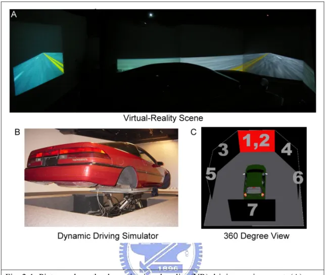
For simulating the real driving environment, a VR based highway-driving environment was developed in our previous studies [30][31]. Fig. 2-1 shows VR based driving environment including a 3-D surrounded scene projected from seven projectors (A, C) and a real car mounted on a 6 DOF Stewart platform (B). The dynamic motion platform provided the kinesthetic stimuli which experienced in the real driving.
2.2
Subjects
Ten volunteers (ages from 19 to 25 years, 7 males and 3 females) with normal or corrected-to-normal vision and with driving license were paid to participate in the experiment. Previous studies [32][33] suggested that drowsiness easily occurs from late night to early morning and during the early afternoon hours. Therefore, all experiments in this study began around one hour after the lunch. Before each session,
participants were required to practice to keep the car at the center of the cruising lane by maneuvering the car with the steering wheel at least for 5 min until reaching satisfactory performance. Each subject had to complete two 60-min sessions on two separated days.
2.3
The lane keeping driving task
For monitoring the driver’s alertness, lane keeping driving task was designed to index the subject’s drowsiness status. Fig 2-2 shows the digitalized highway scene that used in drowsiness experiment. This scene was divided into 256 points and the width of each lane and the car were 60 and 32 points respectively. The refresh rate of highway scene was set at 60Hz, which can properly emulate a car driving at a fixed speed of 100 km/hr on the highway. All scenes were updated according to the displacement of the car and the subject’s wheel handling. The car was randomly drifted away from the center of the cruising lane, which was controlled and triggered from the WTK program, to mimic the consequences of a non-ideal road surface. The inter-deviation intervals were varied from 5 to 10 sec and the car was deviated either left or right with the equal chance. This task required subjects to compensate the drifting by manipulating the steering to keep the car on the center of third cruising lane (from left to right counted). Each subject practiced the driving task until reaching the satisfactory performance after the placement of the EEG cap and electrodes. During the experiment, subjects were instructed to continuously perform the task as best as they could even if they began to feel drowsy. No intervention was made when the subjects was occasionally fell asleep and stopped responding. After such non-responsive periods subjects resumed task performance without experimenter intervention. The onset of each deviation and the subject’s reaction time were
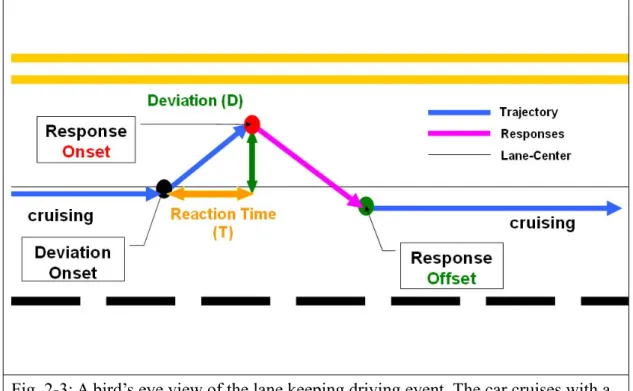
recorded at the rate of 60 times per second via a synchronous pulse marker train that was recorded in parallel by the EEG acquisition system for the further off-line analysis. Fig. 2-3 illustrates the experimental paradigm and the temporal profile of a typical deviation event in the lane-keeping driving task.
2.4
EEG data acquisition
During each driving session, subjects were with a movement-proofed electrode cap with 43 sintered Ag/AgCl electrodes for measuring the electrical activates of the brain and that is the electroencephalogram (EEG). The 43-channel -EEG electrodes were composed by 28channels (from a 30–channel’s 10-20 standard system but excluded the FP1, Fp2) and the hand-made forehead 15 channels (Fig. 2-5). A rectangular 5x3 forehead electrode arrays were embedded on a soft material which is made of high density of ethylene vinyl acetate (EVA) foam (Length x Width: 10cm x 6cm) and the inter-electrode distance was 1.5 cm. The position of channel-12 and -14 were located at the positions corresponded to the Fp1, Fp2 of the 30 channel’s 10-20 standard system. The 15 EEG channel covered the whole forehead region, thus we could collect all signals emitting from the frontal lobe region. Before data collection, the contact impedance of the EEG electrodes was less than 5 kΩ. The EEG activities were recorded and amplified by the SynAmps2 NeuroScan Systems (Compumedics Ltd., VIC, Australia) with the sampling rate of 500 Hz and 32-bit vertical resolution.
2.5
Behavioral data analysis
In each 60-min session, around 200~300 deviation events were recorded. Similar to real-world driving experience, the vehicle did not always return to the same cruising position after each compensatory steering maneuver. Therefore, during each
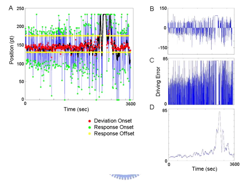
drift/response trial, driving error was measured by maximum absolute deviation from the previous cruising position. Fig 2-4 shows the procedures of behavioral data analysis. The Fig. 2-4A shows the original driving trajectories, and the red, green and yellow dots represent the time occurrences of the deviation onset, response onset and response offset respectively. The driving errors of each session were first computed by subtracting the baseline (the car position before event onset). Second, a threshold (85) was used to correct the different maximum value of drifting to left or right. Third, the temporal profile of the corrected driving errors were smoothed using a causal 90-second square moving-averaged filter advancing at 2-second steps to eliminate variance at cycle lengths shorter than 1–2 minutes since the fluctuates of drowsiness level with cycle lengths were in general longer than 4 minutes (D) [34][35]. Since subjects easily exhibited relative inattention to environments, eye closure, less mobility, slow or worse motor control or responses or decision making [63], the local driving error is varied along with drivers’ alertness conditions. Therefore, we had a drowsiness index: local driving error (LDE). For instance, when the driver was drowsy, the local driving errors were increased. In the contrary, the local driving errors were decreased when the driver was alert.
2.6
EEG data analyses
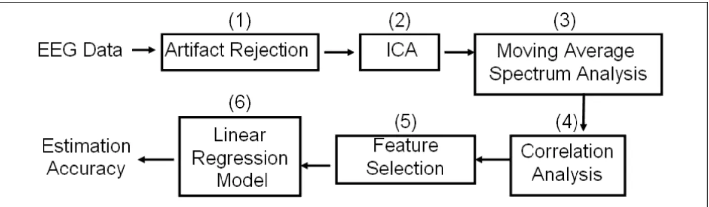
The fig. 2-6 shows the flowchart of EEG data analysis. The detail procedures were described as the followings.
2.6.1
EEG Data pre-processing
with the cut-off frequencies at 50 Hz and 0.5 Hz to remove the line noise, other high-frequency noises and electrogalvanic signals. The filtered EEG signals were screened and rejected grossly data contaminated by other artifacts including muscle contractions the body movement artifacts, and bad channels before the further EEG analysis (fig. 2-7).
2.6.2
Independent Component Analysis
Independent component analysis (ICA) method (fig. 2-8) has extensively applied to blind source separation problem since 1990s [36]-[44]. Subsequent technical reports [45]-[52] demonstrated that ICA is a suitable solution to the problem of EEG source segregation, identification, and localization. Applying ICA algorithm on EEG raw data in drowsiness experiment could remove the EEG artifacts including the eye blinking as well as the eye movements and could further extract EEG sources associated with human drowsiness. In this study, 43-independent components (ICs) were calculated from applying ICA algorithm on 43-channel EEG data. The fig. 2-9 shows the 43 ICs of a single subject (subject 1). The IC-1, -2,-3, -4, -6, -8, -11 were identified as EEG sources and the IC-5, -10, -13, -14, -16, -17, -18, -19, 20, -21, -23, -24, -25, -27, -28, -31, -33, -34, -35, -36, -37, -38, -39, -40, -41, -42, -43 were identified as noise components. The frontal central midline (FCM), occipital-midline (OM) and bi-lateral occipital (BLO) components were selected by visual inspection of scalp topography and then the component signals were used for advancing analysis. In order to extract EEG source related to drowsiness only from forehead, we also applied the ICA algorithm on forehead 15 channels. Although these forehead EEG channel signals were similar on time domain and their topographical locations were very close, ICs related to drowsiness could still be decomposed from these similar channel
signals after applying the ICA algorithm.
2.6.3
Dipole source localization
In order to find the stable and inter-subject consistent sources related to the drowsiness, the FCM and OM ICs were selected from all volunteers. For each IC activation map, we performed an EEG source localization procedure to locate its single dipole. By localizing multiple dipoles independently, we substantially reduced our search complexity and increased the likelihood of efficiently converging on the correct solution. The independent EEG processes and their equivalent dipole source locations were obtained by using the EEGLAB toolbox [53].
2.6.4
Moving-averaged power spectra analysis
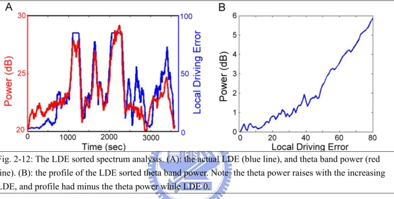
The fig. 2-10 shows the moving-averaged spectral analysis of the extracted 43 ICs/channel data. Signals were first accomplished by using a 750-point Hanning window overlapped with 250-point. The 750-point epochs were further subdivided into several 125-point sub-windows using the Hanning window again advanced by 25-point step. Each 125-point sub-window was zero padded into 256 points and applied by a 256-point fast Fourier Transform (FFT). A moving median filter was then used to minimize the presence of artifacts in all sub-windows. The moving-averaged power spectra were further converted into a logarithmic scale for spectral correlation and driving performance estimation. Each session were consisted of 43 ICs logged power spectra were then estimated across 50 frequencies (from 1 to 50 Hz) stepping at a 2-second (500-point, an epoch) time interval. The fig. 2-12A shows the temporal changes of the theta-band power, which is smoothed using a
causal 90-second square moving-averaged filter advancing at 2-second steps, and the LDE.
2.6.5
Correlation analysis
To select drowsiness-related components, we correlated the smoothed IC power spectrum with the LDE. Since the alertness level was fluctuated with cycle lengths longer than 4 minutes, we smoothed the temporal profile of the power spectra and driving performance with a causal 90-second square moving-averaged filter. The
Pearson’s correlations coefficients between changes in the ICs log power spectrum
and driving performance at each EEG frequencies are expressed as .
The ICs with the highest correlation coefficients among several frequency bands located in FCM and OM were selected for drowsiness estimation. The same correlation estimating processes were also applied on 15 forehead components.
2.6.6
Feature extraction and drowsiness estimation
In this study, we used a multivariate linear regression model [54] to estimate the subject’s LDE based on the power spectra of several signals (FCM, OM, forehead ICs, and forehead channel). The 5-Hz band power with the highest correlation coefficient was selected from each subject as inputs to train the individual linear regression model. For each subject, the ICA unmixing matrix obtained from the training session was applied on testing session which the data were collected in different day. The estimated LDE traces were obtained by multiplying the selected features obtained from the testing session and the linear regression model. The fig. 2-11 shows that the
estimation results of a single subject (subject1). The correlation coefficients between the estimated and actual LDE traces were 0.85 and 0.9 for the within-session testing and the cross-session testing respectively.
2.6.7
LDE sorted spectral analysis
The power changes in theta and alpha bands were sorted according to LDE. The LDEs from 5 to 85 were evenly divided into 80 bins and the corresponded alpha- and theta-band power in each bin was averaged. The fig. 2-12B shows the average LDE sorted theta band power.
2.6.8
Coherence analysis
The EEG coherence is a normalized measurement of the coupling between two signals at any given frequencies [55][56]. The coherence value of each frequency bin was calculated by
, which is the extension of Pearson’s correlation coefficient to complex number pairs. In this equation, f denotes the spectral estimate of two EEG signals x and y for a given frequency bin (
λ
). The numerator contains the cross-spectrum for x and y (f
xy), while the denominator contains the respective autospectra for x (f
xx) and y (f
yy). For each frequency bin (λ), the coherence value (Cohxy) is obtained by squaring the magnitudeof the complex correlation coefficient R. This procedure yields a real number between 0 (no coherence) and 1(maximal coherence). In this study, the coherence of FCM and OM IC signals were evaluated from 20 sessions across 10 subjects.
3.
Results
Previous studies showed that the strongest response related to human drowsiness was mainly found in the occipital lobe with alpha power increases. However, in order to improve the acquisition procedure in the future, brain activities were not only collected with traditional 32 channel electrode cap but also from subjects’ forehead. We first applied ICA on the collected EEG signals (including the 15 forehead channels and the 28 traditional channels) to isolate brain sources. Then, coherence analysis was used to find out the coupling relationship between FCM and OM component.
Two ICA components, FCM and OM, were selected to compare with the 15 forehead components and the 15 forehead channels. The ICA sub-band power of FCM, OM, forehead components and forehead channels were extracted from the first session experiment of each subject. The sub-band powers were then used as features to estimate the driver’s drowsiness state with linear regression model.
In order to investigate the relationship between power changes and LDE, the LDE were then sorted to find out the power change from alert to drowsy. The power changes of FCM, OM, and forehead components were then characterized by comparing their power responses. The following paragraphs showed detailed results.
3.1
OM and FCM ICs clusters
Plenty of brain sources involved in the drowsiness experiments. The ICs were extracted by applying ICA algorithm to 43-channel EEG artifact-free data. According to previous studies, the drowsy-related brain activities were found in the occipital lobe, thus we first focus on the brain activities in this region.
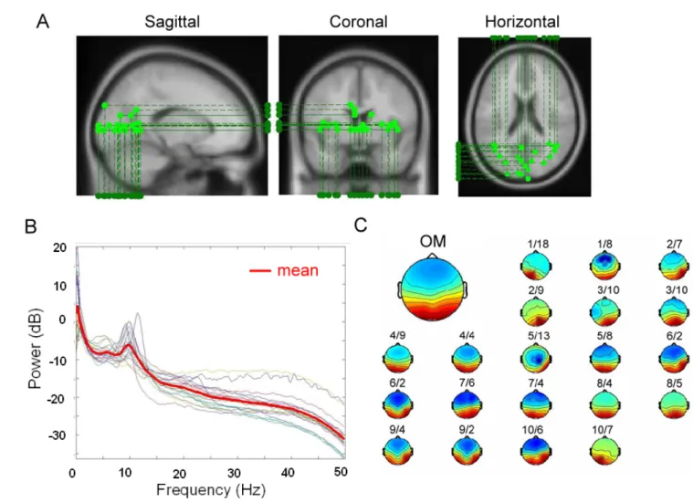
power spectrum, dipole location of OM in all sessions were grouped in one figure. Fig. 3-1 shows the power spectrum, dipole location and scalp topographies of ICA back-projection matrix W-1 of OM components in 20 sessions. Twenty OM components provide strong evidence that EEG source occur on occipital lobe is stable among all subjects during drowsy experiment, and correlation coefficient between each scalp map and mean scalp map ICA back projection matrix W-1 is 0.87±0.2. The spectrum of each OM component and pair correlation coefficient is 0.904±0.6 (panel B). Small scalp map of panel C shows that the OM components appearing in all the 20 sessions, and the bigger scalp topography in the left-upper corner is the scalp map of average ICA back-projection matrix W-1. Note that dipole of OM components mainly located on occipital lobe, but there are four dual-dipoles that belong to bilateral occipital component in Fig. 3-1.
In addition to OM component that activated from alert to drowsy, FCM components were found stable appearing in our twenty sessions (Fig. 3-2). Fig. 3-2C shows the average FCM scalp map and FCM scalp maps appearing in each session, and the correlation coefficient matrix of W-1 is 0.94±0.06. Fig. 3-2B shows the spectrum of each FCM component and pair correlation coefficient is 0.917±0.25. Spectrum profile of OM component had a peak in alpha band, but the spectrum characteristics in FCM had a peak in theta band and 15 Hz. In addition to spectrum and scalp topographies, fig. 3-2A shows the different view point of dipole source, dipoles of FCM component mainly located at the midline of frontal lobe, but some dipoles located near thalamus due to indirect channel locations or experimental setup error. Overall, OM and FCM components were found and having stable profile in dipole location, spectrum and topography during the drowsiness experiment. According to our results, OM and FCM components can be used as EEG features to estimate driver’s drowsiness.
3.2
Coherence between FCM and OM component
In order to figure out the synchronization between FCM and OM ICs, coherence analysis was applied to these two ICs. The coherence value was counted between the one-hour signals from FCM&OM component in each session. Fig. 3-3 illustrates the mean coherence in 1~30 Hz between FCM & OM from 20 sessions, the coherence value donates the coupling degree between two time series. The coherence value in alpha band (around 11Hz) is lower than other frequency band, but higher in theta band (4~7Hz), and the peak appears at 15 Hz. Coherence result shows that phase synchronization in theta band and 15 Hz is higher than alpha band between FCM and OM ICs. Phenomenon appearing in frontal and occipital lobe is similar in theta band.
3.3
Relationship between FCM Component and Forehead
Component
In order to collect more signal from frontal lobe, forehead patch were developed. The 15 forehead components were extracted from the 15 forehead EEG signals. Although these forehead EEG channel signals were similar on time domain and their topographical locations were very close, but ICs related to drowsiness could still be decomposed from these similar channel signals after applying the ICA algorithm.
The 15 forehead components were decomposed from 15 forehead channel EEG signals, and the forehead component with highest correlation coefficient between spectrum and LDE was selected and then back-projected to the 15 forehead channels with matrix W-1. The result of back projection with the forehead component was shown in Fig. 3-4. These 15 color blocks present the ICA back-projection matrix W-1 value of a forehead component, and figure shows that the component weight is higher
in superior way (away from eye) and symmetry in the vertical direction (channel 13). Furthermore, correlation coefficients between forehead and FCM component signals on the time course were calculated (0.64±0.17). In addition to FCM component, correlation coefficient between forehead signal and OM component time series is 0.06±0.04.
The forehead components were proved highly correlated to the FCM components, while the correlation coefficients between forehead components and the OM components are very low. These results suggest that there is a brain source located in frontal lobe response to drowsiness and it can be easily collected from forehead EEG signals.
3.4
LDE Estimation
In last section, we have proved that the forehead components were highly correlated to FCM components and thus can also be used as features to estimate subjects’ cognitive state.
In order to monitor subject’s cognitive state, LDE is an indirect index to measure subject’s cognitive stage. The car in the VR scene was designed to drift from the middle of driving lane to test the subjects’ cognitive response. The distance between the middle of the car and the middle of cruising lane was defined as local driving error, which can be used to study the subjects’ cognitive state. For example, if the subject is alert, the car-drifting can be detected and LDE can be minimized by the subject with the steering wheel. In contrast, LDE will become very large if the subject is drowsy.
We use a least-square multivariate linear regression model to estimate subject’s LDE according to the information obtained from the sub-band power spectra analysis of ICs and EEG channel. The OM and FCM components decomposed from 43-ch
EEG signals, the 15 forehead channels and the 15 forehead components were used as drowsiness-related brain signals in this study. For each signal source, the optimal frequency bands were selected according to the correlation coefficients between ICA power spectrum and LDE in the training session. The single-subject model was trained with the EEG features that extracted from the first session experiment for each subject and then used to estimate subject’s driving performance with the EEG features in second session. The results shown in Table 1 are the correlation coefficients between the estimated driving error and the real LDE acquired in the second session. In reverse, the EEG signals and LDE collected in the second session were used to train the model and the features extracted from the first session signals were used to estimate the driving error. (i.e. S2 est S1)
In Table 1, the averaged correlation coefficient between the estimated driving error and the real driving error is highest (0.89±0.04) when the features were extracted from the OM components, and it’s 0.83±0.07 when FCM features were used. The result suggests that there is another drowsiness-related brain source located in the frontal lobe. Besides, the forehead signals yield better estimation accuracy than FCM component, which means even without complicated application of electrode cap, forehead signals can be used to estimate the subjects’ cognitive state. The correlation coefficients were very similar when the forehead components and the forehead channels were used, the application of ICA thus become unnecessary for this study. In order to investigate the difference between results of four groups, we first applied the Kolmogorov-Smirnov test (KS test) to each group, all groups are not normal distribution, and second we applied the Wilcoxon Signed-Rank test between the groups. The difference between the OM and the other three groups are significant (p<0.05). Furthermore, there is no significant difference between FCM ICs, forehead ICs, forehead channel through the Wilcoxon Signed-Rank test.
According to our results, the OM lobe is the area that most correlated to drowsiness, but frontal lobe features are also good for the estimation of driving performance. These results suggest that we can detect drowsiness by using a single forehead channel and thus save lots of preparation comparing to wearing the electrode cap.
3.5
LDE sorted spectral analysis of ICA components
In order to investigate the brain dynamics corresponding to the transition from alertness (lower LDE) to drowsiness (larger LDE) in the experiments, the ICA log power spectra were sorted according to their LDE. The smoothed results were given in Fig. 3-5.
The sorted LDE values were shown in ascending order in x-axis and the transient frequency band mean power and standard deviation power corresponding to the sorted driving performance values were shown in y-axis. It can be found that the alpha power increased sharply at lower LDE (around 30) and starting decrease latter as ascending driving performance in OM and forehead component. Oppositely, alpha power of FCM increased 2 dB from LDE 5 to 85. Changes in theta band of all components increase from LDE 5 to 85, but OM component have higher increasing power. Power in theta band increased 6 dB from LDE 5 to 85, and this phenomenon can be used to detect driver’s cognitive state from alert to drowsy. In addition, theta band is a better index than alpha band.
4.
Discussion
4.1
Drowsiness detection
In the study, the brain dynamic related to drowsiness during lane keeping driving task recorded by using EEG and VR-based realistic driving environment was investigated. First of all, the signal from occipital lobe is mostly high correlated to drowsiness state, and Fig. 3-1 show that the OM ICs activated in one-hour drowsiness experiment. The correlation are particularly strong at posterior area, which are similar to the result of previous studies in the drowsy experiments [20][22]. In our previous study [57] showed that selecting 2 channel, which was highest drowsiness related, the mean correlation coefficient between estimating and actual driving performance is 0.862±0.072 for within-session testing and 0.882±0.048 for cross-session testing. The accuracy in this study using OM component is 0.89±0.04 is consistent to our previous finding [57]. In addition to OM ICs clusters, that FCM ICs clusters exhibited the power changes in theta band was also suggested highly correlated to the drowsiness [59].
To confirm if the forehead-chanel signals could reflect the activities in the frontal lobe, we compared the LDE sorted alpha and theta power changes of the forehead signals and of the frontal IC clusters decomposed by application of ICA on the 43-channel signals. Results suggested that signals recorded from the forehead channels could full reflect the changes in the frontal regions. In addition, given use signals recorded from one forehead channel could still accurately detect the drowsiness. Results demonstrated that the signals recorded from the forehead channels can directly applied in the drowsiness estimation, and therefore can drastically reduce the data processing time, which means that the drowsiness detection can be more closely to the real time.
4.2
Coupling between FCM and OM ICs clusters.
In order to figure out the phase synchronization between frontal and occipital lobe, we computed the coherence value between FCM and OM components. Computing coherence value between these signals from frontal and occipital lobe were not found in other studies. Fig 3-3 shows the theta band and 15Hz have higher coherence than alpha band. In order to find out the detailed changes between two ICs clusters, power changes in different band in time series was plotted. Fig. 4-4 shows the different band (theta, alpha and 15 Hz) power changes in time course and relative LDE. Note that power change in theta band and 15 Hz in FCM and OM are similar during high LDE (red shading) and low LDE (green shading) period. But OM power changes in alpha band are larger than FCM changes in low LDE period (green shading). Coherence is a method to evaluate the synchronization between two signals; therefore Fig. 4-4 explained low coherence value in alpha band between FCM and OM due to the different power trends.
4.3
EEG phenomenon comparing to other studies
Fig. 3-5 shows that theta band power increased monotonically in the OM and FCM components The alpha band power linearly increased when the LDE less than 30, but the power was decreased when the LDE more than 30 in OM and forehead component. The changes of the alpha band power in our study are opposite to previous studies [61][62][64], which indicated that, alpha power decreases during the transition from wakefulness to sleep onset. We speculated the inconsistency probably due to the different experimental design.
4.4
Comparison of selecting several forehead channels
In order to investigate the number of forehead channel that is sufficient to detect drowsiness. 1~5 channels were selected from forehead channel 11~15. Channels were randomly selecting then used for estimation. Table 2 shows that the accuracy decreased dramatically after using 5 channels (0.69), but it remains above 0.80 using 1~4 channels. This result indicated that using 1 channel or 4 channels didn’t have large different.
5. Conclusions
Drowsiness detection is an important safe issue to the public, but the present detecting system using EEG signals encountered a problem, which this system needs lots of preparation before driving and the driver easily felt uncomfortable and incontinent while wearing electrode cap. Therefore, to develop an easy preparation and comfortable detecting system is great of urgency. In this study, we demonstrated that changes of frontal lobe activities were highly correlated to drowsiness. In the future, the new generation EEG based drowsiness detecting system can directly applied the dry MEMS recording electrodes on the forehead and this detecting system will be able to drastically reduce the drowsiness related injuries and deaths in the real operational environments.
6. References
[1] E. L. Wienner, “Vigilance and inspection”, J. S. Warm (ed.), Sustained Attention
in Human Performance (John Wiley, New York) , 1984, 207±246
[2] G.A. Ryan, “Road traffic crashes by region in western Australia.”, Hartley, L. (Ed.), Fatigue & Driving, 1995, Taylor & Francis, London, pp. 51–57.
[3] M. Shuman, “Asleep at the wheel.” Traffic Safety, January/ February, 1992. [4] D. Royal, “Volume I—Findings report; national survey on distracted and driving
attitudes and behaviours, 2002,” The Gallup Organization, Washington, D.C., Tech. Rep. DOT HS 809 566, Mar. 2003.
[5] D. Chaput, C. Petit, S. Planque, and C. Tarrière, "Un système embarqué de étection de l'hypovigilance," Journées d’études: le maintien de la vigilance dans les Transports,Lyon, France, 1990.
[6] J. Fukuda, E. Akutsu, and K. Aoki, "Estimation of driver's drowsiness level using interval of steering adjustment for lane keeping," JSAE Review, 1995, Society of Automotive Engineers of Japan, vol. 16, pp. 197-199.
[7] R. Grace, V. E. Byrne, D. M. Bierman, J. M. Legrand, D. Gricourt, B. K. Davis, J. J. Staszewski, and B. Carnahan, “A drowsy driver detection system for heavy vehicles,” in Proc. 17th AIAA/IEEE/SAE Conf. Digital Avionics Systems, vol. 2, Nov. 1998, pp. I36/1–I36/8.
[8] C. A. Perez, A. Palma, C. A. Holzmann, and C. Pena, “Face and eye tracking algorithm based on digital image processing,” Proc. IEEE Int. Conf. Systems, Man, Cybernetics, vol. 2, Oct. 2001, pp. 1178–1183.
[9] T. Pilutti and G. Ulsoy, “Identification of driver state for lane-keeping tasks,”
IEEE Trans. Syst, Man, Cybern. A, Syst. Humans, vol. 29, pp. 486–502, Sep.
1999.
[10] J. C. Popieul, P. Simon, and P. Loslever, “Using driver’s headmovements evolution as a drowsiness indicator,” in Proc. IEEE Int. Intelligent Vehi- cles
Symp., Jun. 2003, pp. 616–621.
[11] J. Qiang, Z. Zhiwei, and P. Lan, “Real-time nonintrusive monitoring and prediction of driver fatigue,” IEEE Trans. Veh. Technol., vol. 53, pp. 1052–068, Jul. 2004
[12] R. Grace, V. E. Byrne, D. M. Bierman, J. M. Legrand, D. Gricourt, R. K. Davis, J. J. Staszewski, and B. Carnahan, "A drowsy driver detection system for heavy vehicle," presented at Proceedings of the 17th Digital Avionics Systems
[13] D. F. Dinges, M. Mallis, G. Maislin, and J. W. Powell, "Evaluation of techniques for ocular measurement as an index of fatigue and as the basis for alertness management," National Highway Traffic Safety Administration 1998.
[14] Matsuoka Takayuki, Yokoyama Kiyoko, Mizuno Yasufumi, Takata Kazuyuki “Estimation of Drowsiness While Driving Using Experimentally-derived Time Series of Heart Rate Variability.” Bulletin of Daido Institute of Technology 2000 [15] J.A. Horne, L.A. Reyner, “Counteracting driver sleepiness: effects of napping,
caffeine, and placebo” Psychophysiology 33, 1996, 306–309.
[16] J. A. Stern, D. Boyer, and D. Schroeder, “Blink rate: a possible measure of fatigue,” Human Factors, 1994, vol. 36, no. 2, pp. 285–297.
[17] T.-P. Jung, S. Makeig, M. Stensmo, and T. J. Sejnowski, “Estimating alertness from the EEG power spectrum,” IEEE Trans.Biomed. Eng., 1997, vol. 44, no. 1, pp. 60–69.
[18] S.Makeig and T.-P. Jung, “Changes in alertness are a principalcomponent of variance in the EEG spectrum,” Neuroreport, 1995, vol. 7, no. 1, pp. 213–216. [19] M. Matousek and I. Peters´ en, “A method for assessing alertness fluctuations
from EEG spectra,” Electroencephalography and Clinical Neurophysiology, 1983, vol. 55, no. 1, pp. 108–113.
[20] S. Makeig and M. Inlow, “Lapses in alertness: coherence of fluctuations in performance and EEG spectrum,” Electroencephalography and Clinical
Neurophysiology, 1993, vol. 86, no. 1, pp. 23–35.
[21] J. Qiang, Z. Zhiwei, and P. Lan, “Real-time nonintrusive monitoring and prediction of driver fatigue,” IEEE Trans. Veh. Technol. , 2004, vol. 53, no. 4, pp. 1052–1068.
[22] S. Makeig and T.-P. Jung, “Tonic, phasic, and transient EEG correlates of auditory awareness in drowsiness,” Cognitive Brain Research, 1996, vol. 4, no. 1, pp. 15–25.
[23] Klimesch, W., “EEG alpha and theta oscillations reflect cognitive and memory performance: a review and analysis.” Brain Research Reviews 29, 1999, 169–195.
[24] T.P. Jung, S. Makeig, M. Stensmo, and T.J. Sejnowski, “Estimating alertness from the EEG power spectrum,” IEEE Trans.Biomed. Eng. , 1997, vol. 44, no. 1, pp. 60–69.
[25] S.Makeig and T.P. Jung, “Changes in alertness are a principal component of variance in the EEG spectrum,” Neuroreport, 1995, vol. 7, no. 1, pp. 213–216. [26] P. Parikh and E.Micheli-Tzanakou, “Detecting drowsiness while driving using
wavelet transform,” in Proc. IEEE 30th Annual Northeast on Bioengineering
[27] H.J. Park, J.S. Oh, D.U. Jeong, K.S. Park, “Automated sleep stage analysis using hybrid rule-based and case-based reasoning,” Computers and Biomedical
Research, Volume 33, Issue 5, October 2000, Pages 330-349
[28] C.T. Lin, R.C. Wu, T.P. Jung, S.F. Liang, T.Y. Huang, “Estimating Driving Performance Based on EEG Spectrum Analysis” EURASIP Journal on Applied
Signal Processing, 2005
[29] J.C. Chiou, L.W. Ko, C. T. Lin, C. T. Hong, T. P. Jung, S. F. Liang, and J. L. Jeng, “Using Novel MEMS EEG Sensors in Detecting Drowsiness Application,” 2006 IEEE Biomedical Circuits and Systems Conference (BioCAS 2006), London, United Kingdom, Nov. 29-Dec. 1, 2006.
[30] C. T. Lin, R. C. Wu, T. P. Jung, S. F. Liang, and T. Y. Huang, “Estimating alertness level based on EEG spectrum analysis,” EURASIP J. Appl. Signal
Process. Mar. 2005, vol. 2005, no. 19, pp. 3165–3174.
[31] C. T. Lin, R. C. Wu, S. F. Liang, W. H. Chao, Y. J. Chen, and T. P. Jung, “EEG-based drowsiness estimation for safety driving using independent component analysis,” IEEE Trans. Circuits Syst. I. Dec. 2005, Reg. Papers, vol. 52, no. 12, pp. 2726–2738.
[32] J. Hendrix, “Fatal crash rates for tractor-trailers by time of day,” in Proc.Int.
Truck and Bus Safety Res. Policy Symp. 2002, pp. 237–250.
[33] H. Ueno, M. Kaneda, and M. Tsukino, “Development of drowsiness detection system,” in Proc. Vehicle Navigation and Information Systems Conference (VNIS ’94), 1994, pp. 15–20, Yokohama, Japan, August–September.
[34] T.-P. Jung, S. Makeig,M. Stensmo, and T. J. Sejnowski, “Estimating alertness from the EEG power spectrum,” IEEE Trans. Biomed. Eng. 1997, vol. 44, no. 1, pp. 60–69.
[35] S.Makeig and T.-P. Jung, “Changes in alertness are a principal component of variance in the EEG spectrum,” Neuroreport, 1995, vol. 7, no. 1, pp. 213–216. [36] J. Beatty, A. Greenberg, W. P. Deibler, and J. O’Hanlon, “Operant control of
occipital theta rhythm affects performance, in a radar monitoring task,” Science, 1974, vol. 183, pp. 871–873.
[37] C. Jutten and J. Herault, “Blind separation of sources I. An adaptive algorithm based on neuromimetic architecture,” Signal Process. 1991, vol. 24, pp. 1–10. [38] J. F. Cardoso and A. Souloumiac, “Blind beamforming for non Gaussian
signals,” IEEE Proc. F, 1993, vol. 6, pp. 362–370.
[39] P. Comon, “Independent component analysis — A new concept?,” Signal
[40] A. J. Bell and T. J. Sejnowski, “An information-maximization approach to blind separation and blind deconvolution,” Neural Computat. 1995, vol. 7,pp. 1129–1159.
[41] J. F. Cardoso and B. Laheld, “Equivariant adaptive source separation,” IEEE
Trans. Signal Process. 1996, vol. 45, pp. 434–444.
[42] D. T. Pham, “Blind separation of instantaneous mixture of sources via an independent component analysis,” IEEE Trans. Signal Process. 1997, vol. 44, pp. 2768–2779.
[43] M. Girolami, “An alternative perspective on adaptive independent component analysis,” Neural Computat.1998, vol. 10, pp. 2103–2114.
[44] T. W. Lee, M. Girolami, and T. J. Sejnowski, “Independent component analysis using an extended infomax algorithm for mixed sub-Gaussian and super-Gaussian sources,” Neural Computat. 1999, vol. 11, pp. 606–633.
[45] S. Makeig, A. J. Bell, T. P. Jung, and T. J. Sejnowski, “Independent component analysis of electroencephalographic data,” Advances in Neural Information
Process. Syst.1996, vol. 8, pp. 145–151.
[46] T. P. Jung, C. Humphries, T. W. Lee, S. Makeig, M. J. McKeown, V. Iragui, and T. J. Sejnowski, “Extended ICA removes artifacts from electroencephalographic recordings,” Advances in Neural Information Process. Syst. 1998, vol. 10, pp. 894–900.
[47] T. P. Jung, S. Makeig, C. Humphries, T. W. Lee, M. J. McKeown, V. Iragui, and T. J. Sejnowski, “Removing electroencephalographic artifacts by blind source separation,” Psychophysiology. 2000 Mar;37(2):163-78.
[48] T. P. Jung, S. Makeig, W. Westerfield, J. Townsend, E. Courchesne, and T. J. Sejnowski, “Analysis and visulization of single-trial event-related potentials,”
Hum Brain Mapp. 2001 Nov;14(3):166-85.
[49] A. Yamazaki, T. Tajima, and K. Matsuoka, “Convolutive independent component analysis of EEG data,” in Ann. Conf. SICE, vol. 2, Aug. 2003, pp. 1227–1231.
[50] A. Meyer-Base, D. Auer, and A.Wismueller, “Topographic independent component analysis for fMRI signal detection,” in Proc. Int. Joint Conf. Neural
Networks, vol. 1, Jul. 2003, pp. 601–605.
[51] M. Naganawa, Y. Kimura, K. Ishii, K. Oda, K. Ishiwata, and A. Matani, “Extraction of a plasma time-activity curve from dynamic brain pet images based on independent component analysis,” IEEE Trans. Biomed.Eng., vol. 52, pp. 201–210, Feb. 2005.
[52] R. Liao, J. L. Krolik, and M. J. McKeown, “An information-theoretic criterion for intrasubject alignment of FMRI time series: Motion corrected independent component analysis,” IEEE Trans. Med. Imag., vol. 24, pp. 29–44, Jan. 2005. [53] Delorme, A. and S. Makeig, EEGLAB: an open source toolbox for analysis of
single-trial EEG dynamics including independent component analysis. Neurosci
Methods, 2004. 134(1): p. 9-21.
[54] S. Chatterjee and A. S. Hadi, “Influential observations, high leverage points, and outliers in linear regression,” Statistical Science, Vol. 1, No. 3 (Aug., 1986), pp. 379-393.
[55] D. M. Halliday, J. R. Rosenberg, A. M. Amjad, P. Breeze, B. A. Conway and S. F. Farmer, “A framework for the analysis of mixed time series/point process data–theory and application to the study of physiological tremor, single motor unit discharges and electromyograms.” Prog. Biophys. Mol. Biol., 1995, 64: 237–278.
[56] P. Rappelsberger, and H. Petsche, “Probability mapping: power and coherence analyses of cognitive processes.” Brain Topogr., 1988, 1: 46–54.
[57] C.T. Lin, R.C. Wu, S.F. Liang, W.H. Chao, Y.J. Chen, T.P. Jung, “EEG-Based Drowsiness Estimation for Safety Driving Using Independent Component Analysis,” in IEEE transaction on circuits and system-I: Regular papers, Vol. 52, NO. 12, December 2005
[58] S. Makeig, T. P. Jung, “Tonic, phasic, and transient EEG correlates of auditory awareness in drowsiness.” Brain Res Cogn Brain Res. 1996 Jul;4(1):15-25. [59] L De Gennaro, M Ferrara, G Curcio, R Cristiani, ”Antero-posterior EEG changes
during the wakefulness–sleep transition. ” Clin Neurophysiol.2001 Oct;112(10):1901-11
[60] L. De Gennaro, F. Vecchio, M. Ferrara, G. Curcio, P. Maria Rossini, and C Laudio Babiloni,” Changes in fronto-posterior functional coupling at sleep onset in humans “ J. Sleep Res. (2004) 13, 209–217
[61] W. Dement, N. Kleitman, “Cyclic variations in EEG during sleep and their relation to eye movements, body motility, and dreaming”, Electroencephalogr.
Clin. Neurophysiol. 9(1957) 673–690.
[62] R. D. Ogilvie, I.A. Simons, R. H. Kuderian, T. MacDonald, J. Rustenburg, “Behavioral, event-related potential, and EEG/FFT changes at sleep onset”,
Psychophysiology. 1991 Jan;28(1):54-64.
[63] K. A. Brookhuis, D. De Waard and S. H. Fairclough ,”Criteria for driver impairment”, Ergonomics, 2003, VOL. 46, NO. 5, 433 ± 445
[64] H. Tanaka, M. Hayashi, T. Hori, “Topographical characteristics and principal component structure of the hypnagogic EEG”, Sleep 20, 1997, 523–534
Fig. 2-1: Pictures show the dynamic virtual reality (VR) driving environment. (A): The picture shows the 3D surrounded VR driving scenes. (B) The picture shows a real car mounted on a 6-degree-of-freedom Stewart platform. (C) A schematic picture shows 360 degree VR scene is projected from seven projectors.
Fig. 2-2: The four-lanes road of the VR scene is separated by a median strip and the distance between the left and right sides of the road is equally divided into 255 points (digitized into values 0–255), where the width of each lane and the car is 60 and 32 units, respectively.
Fig. 2-3: A bird’s eye view of the lane keeping driving event. The car cruises with a fixed velocity of 100 km/hr on the VR-based highway scene and every 5-10 sec the car is randomly drifted either to the left or to the right from the cruising position to mimic the non-ideal road surface. Subjects are instructed to steer the vehicle back to the center of the cruising lane as quickly as possible. The duration between
Fig. 2-4: The analysis of driving trajectories. (A) One hour driving trajectories of the subject 7. The red dots represent the occurrences of the car drifting, the green dots represent the response onsets, and the yellow dots represent response offset. (B) The results of the baseline removal from the raw driving trajectories show in the (A). (C) The driving errors derived by getting the absolute values and adjusting values from (B) to
eliminate the diversity of maximum deviation between left and right drifting. (D) The one-hour driving errors are smoothed by a 90-sec square moving-averaged filter advancing at 2-second step, and the result of
Fig. 2-5: Pictures shows the placement and the positions of the forehead 15-channel. (A) The schematic picture showing the placement of forehead 15-channel patch. (B) Photograph shows the arrangement of the hand-made forehead electrode patch. The forehead 15-channel patch is composed by 15 regular wet electrodes (3 rows, 5 columns) manually sewed on a piece of elastic material (size 10 cm by 6 cm), which can be fit on subjects’ forehead for long-term EEG
recordings. The distance between each electrode pair is 1.5 cm.
Fig. 2-6: The flowchart of the EEG signal analysis. (1): A low-pass filter is applied to remove the line noise, extreme high frequencies (>50Hz) noise, and simultaneously remove artifact EEG and behavior data manually. (2) Independent component analysis (ICA) was used to separate EEG brain resource from underlying artifacts. (3) Moving averaged spectral analysis was used to calculate the EEG log power spectrum of each independent component. (4) Correlation analysis was used to choose bands of component correlating to behavior. (5) Four features, FCM, OM, and forehead components as well as forehead channels, which highly correlated with LDE, are
selected. (6) Linear regression models are built based on changes of EEG power and LDE from training session of the individual subject, and then the model is evaluated by continuously estimating the individual subject’s LDE in the test session.
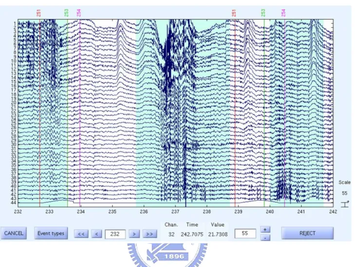
Fig. 2-7: The picture shows the identified artifacts, which generated by the muscle contraction, eye-movement, eye blinking and bad channels, and the artifacts and their corresponded behavioral signals (channel 44) are rejected before the furthering signal process.
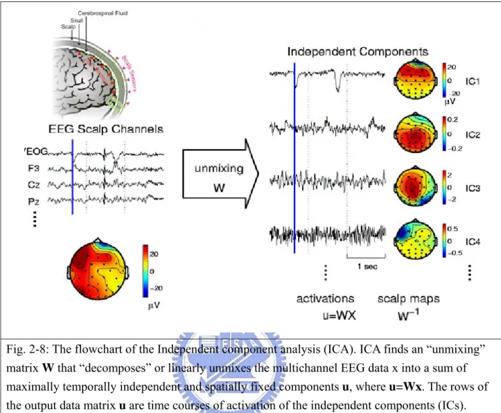
Fig. 2-8: The flowchart of the Independent component analysis (ICA). ICA finds an “unmixing” matrix W that “decomposes” or linearly unmixes the multichannel EEG data x into a sum of maximally temporally independent and spatially fixed components u, where u=Wx. The rows of the output data matrix u are time courses of activation of the independent components (ICs).
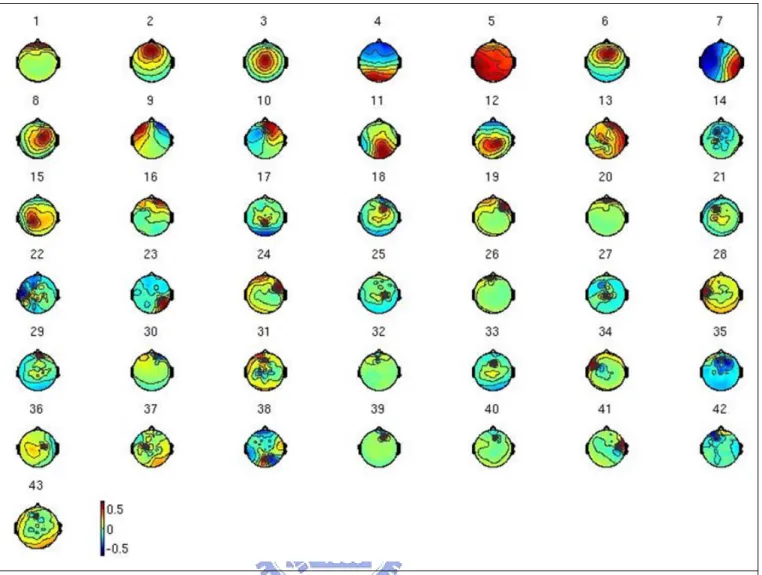
Fig. 2-9: The scalp topographies of ICA weighting matrix W by spreading each Wij into the plane of
the scalp corresponding to the jth ICA components based on International 10-20 system. 43
components are listed above, and the frontal central midline (FCM) and occipital midline (OM) components are selected according to scalp map.
Fig. 2-10: The flowchart of the time-frequency analysis. The EEG signals of the extracted ICA components are first applied by a 750-point Hanning window with 250-point overlap. The 750-point epochs are further subdivided into several 125-point Hanning sub-windows advanced at the step of 25 points. Each 125-point frame is zero padded into 256 points for the 256-point fast Fourier transform (FFT). The frequency resolution of the resultant power-spectrum density is around 1Hz. A moving median filter was used in 750-poing window. Then, the log power spectrum is smoothed by a casual 90-second square moving-filter advancing at 2-second steps.
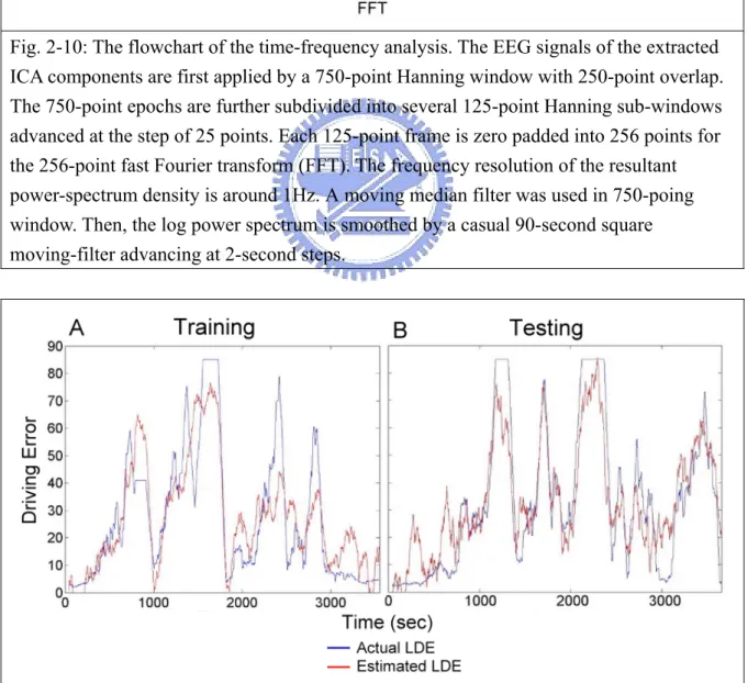
Fig. 2-11. Pictures show the actual (blue lines) and estimated LDE (red lines) by using the linear regression model in the training (A) and testing (B) sessions from the subject 1. The
local driving errors are estimated by a linear regression model with the log power spectra at frequency bands 4 ~ 8 Hz of forehead component, which are known to well correlated with LDE). Note: the results show that the estimated LDE are highly correlated with the actual LDE in both testing (corr coeff. =0.85) and training sessions (corr coeff. =0.9).
Fig. 2-12: The LDE sorted spectrum analysis. (A): the actual LDE (blue line), and theta band power (red line). (B): the profile of the LDE sorted theta band power. Note: the theta power raises with the increasing LDE, and profile had minus the theta power while LDE 0.
Fig. 3-1: Equivalent dipole source location, spectra, and the scalp maps of the occipital component across 20 sessions from 10 subjects. (A): locations of equivalent dipole source and their projection onto average brain images. (B): the power spectra across 20 sessions and the grand mean of the power spectrum (red line). The spectrum correlation coefficient between each session is 0.87±0.2. (C) The topography maps of the occipital component across the 20 sessions. The top left inset shows the grand mean of the scalp topography. The averaged correlation coefficient of the pair component W-1 matrix is 0.90±0.06.
Fig. 3-2: Equivalent dipole source location, spectra, and the scalp maps of the occipital component across 20 sessions from 10 subjects. The man of the pair spectrum correlation coefficient is 0.917±0.05. The averaged correlation coefficient of pair component W-1 matrix is 0.94±0.06. Panels as Fig. 3-1.
Fig 3-3: The coherence between the frontal and the occipital component across 20 sessions. Note: the higher coherences are observed in the delta, theta and low beta band.
Fig. 3-4. The grand means of the frontal component (A) and the forehead component (B). The ICA algorithm is applied to 15 forehead channels and 43 channels (30 channels on cap and 15 forehead channels) respectively, then the correlation coefficient of these two component signals is further evaluated. In each session the forehead component is selected by the highest correlation coefficient with frontal or occipital component. Results show that the forehead component is highly correlated (0.64±0.17) with frontal component than that with the occipital component (0.06±0.04). In addition, the average component weight of chosen forehead
component is symmetric to five columns and having more weight on superior row, thus these highest weight channel can be used instead of forehead component if we didn’t have enough channels to decompose the drowsiness-related component.
Signal Subject(Session) OM FCM Forehead channel Forehead component Subject 1 ( S1 est S2) .83 .82 .87 .88 ( S2 est S1) .92 .91 .94 .90 Subject 2 ( S1 est S2) .78 .91 .89 .84 ( S2 est S1) . 86 .85 .78 .79 Subject 3 ( S1 est S2) . 93 .89 .90 .75 ( S2 est S1) . 89 .92 .91 .81 Subject 4 ( S1 est S2) . 87 .76 .91 .88 ( S2 est S1) . 84 .78 .86 .74 Subject 5 ( S1 est S2) .94 . 86 .94 .89 ( S2 est S1) . 83 .73 .91 .88 Subject 6 ( S1 est S2) .86 .77 .87 .85 ( S2 est S1) . 85 .88 .81 .82 Subject 7 ( S1 est S2) .87 .90 .81 .83 ( S2 est S1) . 94 .87 .93 .89 Subject 8 ( S1 est S2) .93 .83 .92 .89 ( S2 est S1) .87 .92 .84 .80 Subject 9 ( S1 est S2) .90 .75 .88 .85 ( S2 est S1) .86 .73 .88 .85 Subject 10 ( S1 est S2) .94 .69 .93 .84 ( S2 est S1) .87 .78 .86 .73 Mean ( SD ) 0.89 (0.04) 0.83(0.07) 0.88(0.04) 0.83(0.05)
Fig 3-5: The grand mean and the standard error (SD) of the LDE sorted theta (A) and alpha (B) band power from the forehead (black line), FCM(blue line), and OM (red line) component. Note: the theta band power increases monotonically with the driving error. The maximal theta band power is in the occipital component and the powers are around 3 dB attenuated in the frontal and forehead components.
Number of channel Subject(Session) 1 2 3 4 5 Subject 1 ( S1 est S2) .87 .85 .83 .8 .61 ( S2 est S1) .94 .94 .92 .91 .89 Subject 2 ( S1 est S2) .89 .89 .81 .79 .73 ( S2 est S1) .78 .75 .70 .68 .59 Subject 3 ( S1 est S2) .90 .90 .89 .85 .73 ( S2 est S1) .91 .91 .90 .88 .83 Subject 4 ( S1 est S2) .91 .93 .92 .91 .79 ( S2 est S1) .86 .86 .85 .85 .80 Subject 5 ( S1 est S2) .94 .92 .91 .91 .8 ( S2 est S1) .91 .94 .93 .9 .56 Subject 6 ( S1 est S2) .87 .85 .80 .77 .7 ( S2 est S1) .81 .81 .79 .67 .51 Subject 7 ( S1 est S2) .81 .83 .83 .82 .78 ( S2 est S1) .93 .91 .9 .84 .72 Subject 8 ( S1 est S2) .92 .91 .89 .87 .86 ( S2 est S1) .84 .85 .74 .70 .67 Subject 9 ( S1 est S2) .88 .84 .81 .8 .33 ( S2 est S1) .88 .88 .84 .84 .78 Subject 10 ( S1 est S2) .93 .85 .87 .46 .41 ( S2 est S1) .86 .81 .84 .80 .75 Mean ( SD ) 0.88(0.04) 0.87(0.05) 0.84(0.06) 0.80(0.1) 0.69(0.14)