卡曼濾波器應用於永磁同步馬達無感測控制之研究

國

立

交

通

大

學

電機資訊學院 電機與控制學程

碩

士

論

文

卡曼濾波器應用於永磁同步馬達無感測控制之研究

Sensorless Control of Permanent Magnet Synchronous Motors Using

Kalman Filter Theory

研 究 生：葛育中

指導教授：鄒應嶼 博士

卡曼濾波器應用於永磁同步馬達無感測控制之研究

Sensorless Control of Permanent Magnet Synchronous Motors Using

Kalman Filter Theory

研 究 生：葛育中 Student: Yu-Chung Ko

指導教授：鄒應嶼 博士 Advisor: Dr. Ying-Yu Tzou

國 立 交 通 大 學

電機資訊學院 電機與控制學程

碩 士 論 文

A Thesis

Submitted to Degree Program of Electrical Engineering Computer

Science

College of Electrical Engineering and Computer Science

National Chiao Tung University

in Partial Fulfillment of the Requirements

for the Degree of

Master of Science

in

Electrical and Control Engineering

June 2004

Hsinchu, Taiwan, Republic of China

授權書

(博碩士論文) 本授權書所授權之論文為本人在＿交通大學＿＿大學(學院)＿電機與控制＿＿系所 ＿＿＿＿＿＿＿組＿＿九十二＿＿學年度第＿二＿學期取得＿碩＿士學位之論文。 論文名稱：＿＿卡曼濾波器應用於永磁同步馬達無感測控制之研究＿＿＿＿ 1.□同意 □不同意 本人具有著作財產權之論文全文資料，授予行政院國家科學委員會科學技術資料中 心、國家圖書館及本人畢業學校圖書館，得不限地域、時間與次數以微縮、光碟或 數位化等各種方式重製後散布發行或上載網路。 本論文為本人向經濟部智慧財產局申請專利的附件之一，請將全文資料延後兩年後 再公開。(請註明文號: ) 2.□同意 □不同意 本人具有著作財產權之論文全文資料，授予教育部指定送繳之圖書館及本人畢業學 校圖書館，為學術研究之目的以各種方法重製，或為上述目的再授權他人以各種方 法重製，不限地域與時間，惟每人以一份為限。 上述授權內容均無須訂立讓與及授權契約書。依本授權之發行權為非專屬性發行權利。 依本授權所為之收錄、重製、發行及學術研發利用均為無償。上述同意與不同意之欄位 若未鉤選，本人同意視同授權。 指導教授姓名： 研究生簽名： 學號： （親筆正楷） （務必填寫） 日期：民國 九十三 年 月 日 2本授權書請以黑筆撰寫並影印裝訂於書名頁之次頁。 3授權第一項者，所繳的論文本將由註冊組彙總寄交國科會科學技術資料中心。 4本授權書已於民國 85 年 4 月 10 日送請內政部著作權委員會（現為經濟部智慧財產 局）修正定稿。 5本案依據教育部國家圖書館 85.4.19 台(85)圖編字第 712 號函辦理。

國 立 交 通 大 學

論 文 口 試 委 員 會 審 定 書

本校 電機資訊學院專班

電機與控制

組 葛育中 君

所提論文

合於碩士資格水準、業經本委員會評審認可。

口試委員：

指導教授：

班主任：

中 華 民 國 年 月 日

卡曼濾波器應用於永磁同步馬達無感測控制之

研究

學生：

葛育中

指導教授

：鄒應嶼 博士

國立交通大學電機資訊學院 電機與控制學程﹙研究所﹚碩士班

摘

要

永磁同步馬達近年來廣泛應用於資訊家電、自動控制、電動車輛等各種領域，是各 種馬達中成長最快速的，其原因主要是具有高效率，體積小及高扭力。在某些應用如壓 縮機，環境極差無法使用位置感測器(光學編碼器或霍爾元件)及負載較固定且較不要求 快速響應時，無感測器的控制器便有機會使用，可以省下許多感測器的費用，更可以增 加系統的信賴度。本論文利用目前已量產且廉價(低於10塊美金)的TI TMS320LF2407A 16位元DSP及搭配愛德利科技的內插式永磁同步馬達來實現無感測控制。無感測控制的 方法很多，以方波馬達來說感測其反電動勢已行之有年且市場已有現成專門的微處理器 及IC，而本論文是研究此最佳估測器Kalman Filter應用於弦波馬達無感測控制之可行性。

在模擬及實驗中採用了馬達於靜止座標系的動態方程式作為extended Kalman filter (EKF)使用之模型。實驗結果顯示在EKF開路時轉子位置估測值與實際值最大誤差約為 20度，而速度估測可藉由調整反電勢參數得到。實驗結果也顯示了使用TMS320LF2407A 執行整個估測所花費的時間不到100us，証實此顆定點DSP足以用來實現EKF於永磁弦波 同步馬達無感測控制。

Sensorless Control of Permanent Magnet Synchronous Motors

Using Kalman Filter Theory

Student：

Yu-Chung Ko

Advisors：

Dr. Ying-Yu Tzou

Degree Program of Electrical Engineering Computer Science

National Chiao Tung University

ABSTRACT

The number of permanent magnet synchronous motors (PMSM) is constantly growing in the industrial and automotive fields annually largely owning to their high efficiency, small size and high torque. In some applications like compressors or air conditioners, using PMSM with position sensors is extremely difficult. In other applications such as the rigorous environments where the fast response is not required, the sensorless control can be applied. TI TMS320LF2407A is adapted in this investigation owing to its low cost (i.e., less than US$10), rapid calculation (up to 40 MIPS) and the fact that it is already in mass production. The motor for the experiment comes from the AM series motor of Adlee Powertronics Co., LTD. Among the many sensorless control methods available include, the brushless DC motors (BLDCM), utilizing the zero crossing of its back EMF are the easiest and least expensive way of achieving sensorless control. In this thesis, researching the possibility of using Kalman filter with PMSM sine-wave motors is the major study issue. This investigation examines the feasibility of using Kalman filters with PMSM sine-wave motors.

The motor dynamic equations in the stationary frame have been adopted for the EKF in the simulations and experiments. The experimental results reveal that the maximum error between the estimated rotor position and actual one in the steady state is 20 degrees in EKF opened-loop mode, and the estimated speed can be derived by adjusting the back EMF parameter of the dynamic equations. The results also shows that the total program execution period is less then 100us using TMS320LF2407A, and it has revealed this fixed-point DSP is capable of implementing the sinusoidal-excited sensorless control of the PMSM using the EKF theory.

誌

謝

真是一段漫長的歲月啊! 五年的光陰中經歷了許多困難與挑戰，但一切都值得。雖 然沒有完成預期的目標但從實驗的過程中倒是獲益良多。許多人告訴我幹麻虐待自己， 隨隨便便混過就好了，其實怎知會有如此多的挑戰，當初只是好奇想了解罷了。試想若 當初不作此決定現在可能會覺得碩士的歷練不過爾爾。回憶起來過程永遠是最甜美的。 如同當兩年大頭兵，當時會覺得真不是人過的日子，但現在想起來會覺得那是一段值得 一提甚至是可炫耀的回憶。 公司在我求學過程中提供了不少的幫助，尤其是實驗的設備，但實務的經驗與驗證 更幫助我在實現理論時有更高的成功機會，我想這是在職生的優勢。同伴是不可或缺的 一環，實驗室的栩永，光耀及振宇的熱心協助讓我銘記於心。 畫龍點睛的部份要歸功於指導老師應嶼教授了。他在口試前最後的幾個月中讓我體 驗到如何做好研究，那就是你不需要一次解決所有問題，只要專注於一個部份並將其徹 底研究便是一份好的論文，如果我能更早體認這點相信現在的論文會更有水準。最後感 謝口試委員們的指正與建議讓我能順利完成本論文。

Table of Contents

Abstract (Chinese)………..…...……...i

Abstract (English)………...……...…..ii

Acknowledgement………...…….iii

Table of Contents ...iv

List of Tables………...…...vi

List of Figures ...vii

Abbreviation and Symbols ……….x

Chapter 1 Introduction………...… 1

1.1. Research motivation………...…... 1

1.2. Description of experimental testing bench………..……... ..2

1.3. The research goals and system overview………..……... 4

1.4. Dissertation organization...5

Chapter 2 Modeling and Parameters Measurement of A Permanent Magnet Synchronous Motor...7

2.1. Machine model in arbitrary d-q reference frame...7

2.2. Ld and Lq measurement...15

Chapter 3 Kalman Filter Estimator for A PMSM... 16

3.1. Kalman filter on rotor reference frame for a PMSM... 17

3.2. Kalman filter on stator reference frame for a PMSM... 20

3.3. Selection of the time-domain machine model... 23

Chapter 4 Simulations of EKF... 24

4.1. The steps of the discretized EKF algorithm on stator reference frame... 26

4.2 Matlab/simulink simulation of the EKF... 29

4.2.1 Description of the function blocks... 29

4.2.2 Description of the motor simulink model in stator reference frame... 31

4.2.3 Description of the EKF simulink model in stator reference frame... 34

4.3 Simulation results... 37

Chapter 5 Software Implementation of Kalman Filter Theory Estimating Speed and Position ...51

5.1. Scaling for variables ...51

5.1.2. Scaling for EKF models ...54

5.1.3. Scaling for covariance matrices and Kalman gain K ...56

5.2. Software flowchart of the control algorithm ...57

5.3. Software flow chart of EKF ...59

5.4. Assembly language implementation ...60

5.5. Quasi floating point method ...62

5.6. Timing analysis of the EKF...64

5.7. Memory requirements of the codes ...66

Chapter 6 Experimental Results ...67

6.1. Method 1: Flux saturation ...67

6.2. Method 2: Rotor alignment ...73

6.3. Experimental results of EKF ...75

Chapter 7 Conclusions ...82

Appendix ...83

References ...84

List of Tables

Table 5.1 Software execution time...64 Table 5.2 EKF execution time...65 Table 5.3 Memory requirements of the codes ...66

List of Figures

Fig. 1.1 Experimental testing bench ...3

Fig. 1.2 Block diagram of the sensorless control ...4

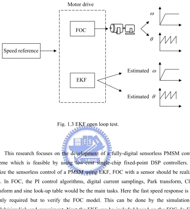
Fig. 1.3 EKF open loop test ...5

Fig. 2.1 Arbitrary d-q reference frame ...7

Fig. 2.2 Equivalent circuit of a PMSM ...13

Fig. 2.3 Interior magnet type rotor L_d ≠ L_q ...14

Fig. 2.4 Surface mount type rotor Ld=Lq=Lss ...14

Fig. 2.5 Ld and Lq measurement ...15

Fig. 3.1 Structure of EKF ...16

Fig. 3.2 Rotor reference frame ...17

Fig. 3.3 Stator reference frame ...20

Fig. 4.1 PMSM with EKF simulink model ...29

Fig. 4.2 PMSM Simulink model in stator reference frame ...31

Fig. 4.3 The EKF model on stator reference frame ...34

Fig. 4.4 White noises ...34

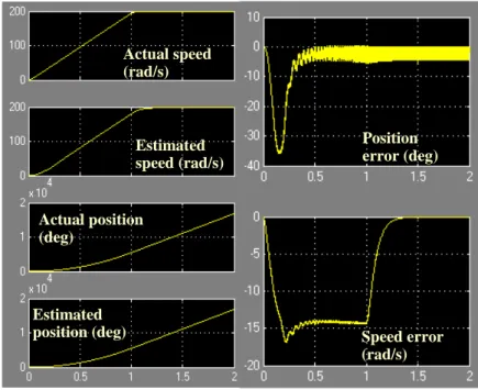
Fig. 4.5 Speed reference = 200 rad/s with EKF open ...37

Fig. 4.6 Speed reference = 200 rad/s with EKF closed ...37

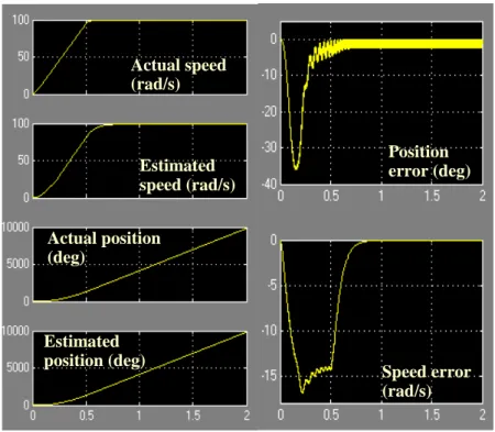
Fig. 4.7 Speed reference = 100 rad/s with EKF open ...38

Fig. 4.8 Speed reference = 100 rad/s with EKF closed ...38

Fig. 4.9 Speed reference = 50 rad/s with EKF open ...39

Fig. 4.10 Speed reference = 50 rad/s with EKF open ...39

Fig. 4.11 Speed reference ...40

Fig. 4.12 Speed response and rotor position without load ...40

Fig. 4.13 Speed response and rotor position with load 0.1N-m at t = 1.5 seconds ...41

Fig. 4.14 Torque response with load 0.1N-m at t = 1.5 seconds ...41

Fig. 4.15 Current response with load of 1.5 N-m at t = 1.5 seconds ...42

Fig. 4.16 Speed response and rotor position using EKF ...43

Fig. 4.17 Current response using EKF in no load condition ...45

Fig. 4.18 Torque response without load using EKF ...45

Fig. 4.20 Speed response and rotor position with load 0.1 N-m using EKF ...47

Fig. 4.21 Torque response using EKF with load 0.1 N-m ...47

Fig. 4.22 Current response using EKF with load 0.1 N-m ...48

Fig. 4.23 Rotor position accumulated error and speed error using EKF with load 0.1 N-m ...48

Fig. 4.24 Speed and rotor position response without load using EKF ...49

Fig. 4.25 Rotor position and speed error without load using EKF ...49

Fig. 5.1 Current scaling ...52

Fig. 5.2 Speed scaling for a 2000 PPR encoder ...53

Fig. 5.3 Position scaling of a 4 pole motor for a 2000 PPR encoder ...54

Fig. 5.4 Software flowchart of the control algorithm ...58

Fig. 5.5 Software flowchart of EKF ...59

Fig. 5.6 Software flowchart of EKF ...63

Fig. 6.1 2 poles PMSM rotor position ...67

Fig. 6.2 Inductance curve ...68

Fig. 6.3 Detecting rotor step 1 ...68

Fig. 6.4 Detecting currents ...68

Fig. 6.5 Six power switches ...69

Fig. 6.6 Detecting rotor step 2 ...69

Fig. 6.7 Detecting rotor step 3 ...70

Fig. 6.8 Detecting current wave forms ...70

Fig. 6.9 Rotor position “5” ...71

Fig. 6.10 Rotor position “1” ...71

Fig. 6.11 Rotor position “3” ...71

Fig. 6.12 Rotor position “2” ...71

Fig. 6.13 Rotor position “6” ...72

Fig. 6.14 Rotor position “4” ...72

Fig. 6.15 Detecting current wave forms on DC bus ...72

Fig. 6.16 Detecting current wave forms on motor phases ...73

Fig. 6.17 Time scaled aligning current wave forms ...74

Fig. 6.18 Aligning current wave forms ...74

Fig. 6.19 Host communication software ...75

Fig. 6.20 Actual rotor position ...76

Fig. 6.22 Error between actual rotor position and estimated one ...77

Fig. 6.23 Enlarged wave form of Fig. 6.22...………78

Fig. 6.24 Actual sin(θ) ...79

Fig. 6.25 Estimated sin(θ) ...79

Fig. 6.26 Error between actual sin(θ) and estimated one ...79

Fig. 6.27 Estimated speed ω_e=550 RPM. Q (3, 3) =0.06...79

Fig. 6.28 Estimated speed ω_e=550 RPM. Q (3, 3) =2 ...79

Fig. 6.29 Actual I_α ...80

Fig. 6.30 Estimated I_α ...80

Fig. 6.31 ActualI_α − estimatedone ...80

Abbreviation and Symbols

ω Angular frequency of q or d-axis

r

ω Angular frequency of rotor

θ Angle between q-axis and stator a axis

r

θ Angle between rotor a axis and stator a axis

p _{Differential operator,} dt

d

abc s

V Stator three phase voltages

0

qd s

V Stator voltages on d-q reference frame

αϕ s

V Stator voltages on αβ reference frame

abc s

λ Stator three phase flux linkage 0

qd s

λ Stator flux linkage on d-q reference frame

abc ss

L Stator three phase self inductance

abc sr

L Mutual inductance between stator and rotor

ls

L Leakage inductance

s

L Stator magnetizing inductance

abc s

r Stator three phase resistance

abc r

r Rotor three phase resistance

abc s

i Stator three phase current

αβ s

i Stator current on αβ reference frame

abc r

i Three phase rotor current

1 |k−

k e

θ The estimated kth θ due to the k-1 stage

1 |k−

k e

Chapter 1

Introduction

In this thesis, the Kalman filter theory is used to estimate the rotor position and speed of a sinusoidal-excited permanent magnet synchronous motor (PMSM) instead of a real position sensor such as incremental encoder or Hall sensor. A sine wave synchronous motor with interior-magnet-rotor-type motor is chosen for the experiment and the developed sensorless PMSM control scheme has been realized by using a single-chip fixed-point DSP controller TMS320F2407A. This thesis shows that although Kalman filter theory is complicated in mathematical manipulation and time-consuming in calculation for the sensorless estimation of a PMSM motor, however, it is still feasible to be implemented by using a single-chip fixed-point DSP with 40 MIPS execution speed. This thesis focuses on the design of an extended Kalman filter in estimation of the rotor position of a PMSM motor and realization issues of the Kalman filter based sensorless control scheme.

1.1. Research motivation

Energy conservation is becoming increasingly important. Motor power consumption occupies a large part of industrial energy use, explaining why most industrialized countries must establish strict laws to save energies. In the automotive filed, increasing numbers of motors are used in vehicles for mechanisms, like water pumps, steering, brake systems. Important reasons for this practice include the need to be environmentally friendly by increasing the ratio of distance per liter of fuel and the desire to keep costs down.

From above, a permanent magnet synchronous motor (PMSM) is the best choice for the application. Although some motor performance may be lost, sensorless control remains practical for applications such as air conditioners, refrigerators, fans and water pumps. While most sensorless control relies heavily on computation, in this decade digital signal processors have made it possible at low cost option. The cheapest 16-bit DSPs are the series of TI’s TMS320LF240x which deliver a good performance up to 40 MIPS. This thesis proposes a way of using TMS320LF2407A to achieve sensorless vector control for PMSMs.

can function efficiently for the sensorless control of a PMSM using the floating-point DSP, WEDSP-32C. The advantages are that the phase voltage transducers are eliminated, and thus simplifying the drive and reducing the cost. In [2], the Texas Instrument (TI) reveals how the EKF works for sensorless vector control of an induction machine. The EKF appears to be a universal solution for a sensorless control of any motor just to modify the motor state equations. According to Tatematsu, Hamad and Uchida [3], this method requires all the information from the PMSM including rotor resistances and d-q inductances with measured phase voltages and currents to estimate speed and position, which could be heavily affected due to the motor parameters and measuring noises especially at low speed. A reduced order observer which uses two special inputs to linearize the non-linear model of a PMSM is introduced [4]. The load torque is set to zero for simplification and no load information is mentioned for the experiment.

Extensive applications have been found by using the EKF algorithms in estimation of rotor position and speed in various sensorless motor drives [5]-[8]. As well known the Kalman filter is a recursive optimum-state estimator which means that as long as the required mathematical model is available, the optimum solution can be achieved. The modeling and parameters measurement techniques of sinusoidal PM synchronous motors can be found in [9]-[14], therefore, the state equations can be derived without difficulty, and this is a key step in employing EKF theory in sensorless motor control.

1.2. Description of experimental testing bench

RS232 interface has been established to communicate with a personal computer to get inputs like speed, torque, PI gain, covariance matrices for the EKF and aligning the rotor. RS232 can also output motor and drive status like speed response, current response and software parameters which makes debugging and tuning easier. The power source is a transformer with adjustable output and the motor for testing is attached with a 2000 pulse incremental encoder. Before the EKF is applied, the field-oriented control (FOC) should be rigorously tested with a real encoder. Another motor is used as a resistive load instead of a servo motor to reduce the noises. JTAG is used for downloading the codes and debugging. The taco generator can be used to observe the speed response in real time with 30V/1000 rpm.

Motor for testing Motor for load Transformer JTAG of TMS320LF2407A Incremental encoder RS232 communication with PC

Motor drive Taco

generator

1.3. The research goals and system overview

DC bus voltage

The EKF is based on field-oriented control as indicated in Fig. 1.2. Idref is preset to zero for the maximum torque output. There are four inputs for the EKF, that are voltage and current feedbacks expressed on αβ frame. and are used instead of the real feedbacks. In fact, voltage measurements are affected by the modulation noise and there must be phase lag due to filtering and the PWM carrier frequency is small with respect to the electrical time constant of the motor so the reference voltage and generated by the current regulator are used instead. The voltage transducers for measuring motor phase voltages can be eliminated as well.

ref

V_α V_βref

ref

V_α Vβref

PI speed

regulator PI current regulator

αβ abc αβ dq EKF Idref=0 ref V_β ref V_α ω _{PMSM Load} Iqref α i β i d i q i Encoder signal Estimated θ_e SVPWM a i b i Estimated ω_e Encoder signal

This research focuses on the development of a fully-digital sensorless PMSM control scheme which is feasible by using low-cost single-chip fixed-point DSP controllers. To realize the sensorless control of a PMSM using EKF, FOC with a sensor should be realized first. In FOC, the PI control algorithms, digital current samplings, Park transform, Clark transform and sine look-up table would be the main tasks. Here the fast speed response is not mainly required but to verify the FOC model. This can be done by the simulation of Matlab/simulink and experiment. Next the EKF can be included based on the FOC. In EKF algorithm, the nonlinear model of the motor, matrices calculation using a fixed-point DSP which is the most complex part would be the primary tasks. An open loop test as indicated in Fig.1.3 is performed first to observe the estimated speed and position. After the actual and estimated shaft speed and position have been matched, the EKF can supplant the incremental encoder to achieve the sensorless control for a PMSM.

1.4. Dissertation organization

Chapter 1 introduces the motor applications in the industrial and automotive fields Speed reference FOC EKF ω θ Estimated ω Estimated θ Motor drive

particularly the PMSM together with the advantages provided by sensorless control.

Chapter 2 derives the dynamic model of a PMSM on the arbitrary rotating d-q frame. The dynamic model is easily mounted on the stationary frame via the rotating d-q frame. Understanding the FOC, EKF and d-q inductance measurement is of fundamental importance.

Chapter 3 introduces the EKF algorithm as applied to the parameter estimation of a PMSM. This chapter includes the nonlinear model for the EKF and the recursive steps for calculating the optimum solution.

Chapter 4 summarizes the simulation results for both FOC and the EKF using Matlab/simulink. The function blocks are illustrated in detail.

Chapter 5 illustrates the software realization using assembly language including how the macros reduce the execution time and simply the software structures. Scaling, software flowchart and timing analysis are also demonstrated clearly.

Chapter 6 details the experiment results including the detection of the initial rotor position, rotor alignment and the EKF estimation results. The detection of the initial rotor position identifies the rotor position within 60 electrical degrees and the rotor alignment forces the rotor to stay at a known position. These two approaches help start the motor successfully.

Chapter 2

Modeling and Parameters Measurement of A Permanent

Magnet Synchronous Motor

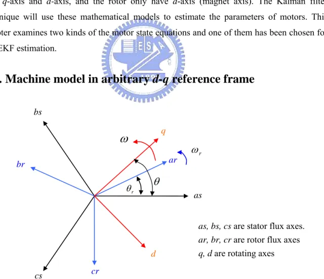
In the control of a sinusoidal PMSM, the most commonly adopted control schemes are the field-oriented vector control (FOC) and direct torque control (DTC). These decoupling control schemes can decouple those nonlinear coupled physical variables to linear decoupled pseudo variables. A PMSM under well decoupled FOC control can behave just like an external excited dc motor, within base speed control range, the developed torque is proportional to the phase current. It decomposes complicated 3-phase stator current vectors into q-axis and d-axis, and the rotor only have d-axis (magnet axis). The Kalman filter technique will use these mathematical models to estimate the parameters of motors. This chapter examines two kinds of the motor state equations and one of them has been chosen for the EKF estimation.

2.1. Machine model in arbitrary d-q reference frame

bs q

ω

r

ω

ar br

θ

r θ as

as, bs, cs are stator flux axes. ar, br, cr are rotor flux axes q, d are rotating axes d

cr

cs

To realize how the field-oriented control works, here below are the motor stator and rotor phasers. “as”, “bs” and “cs” mean a , b and c phase of a motor stator and “ar”, “br” and “cr” mean a , b and c phase of a motor rotor respectively. Each of them means the force vector caused by the stator current and rotor current (magnets). “q” and “d” axes are orthogonal and at arbitrary position.To control a PMSM as a DC motor, those phasers need to project onto the arbitrary d-q frame, that is, three-phase to two-phase transformation.

To simplify mathematical model deriving, assume that (1) The air gap is even,

(2) The magnetic circuit is linear,

(3) The stator winding is arranged to generate sinusoidal inductive voltage.

Now, project those phasers onto d-q reference frame, we need three phase to two phase transformation as below: ⎥ ⎥ ⎥ ⎥ ⎥ ⎥ ⎥ ⎦ ⎤ ⎢ ⎢ ⎢ ⎢ ⎢ ⎢ ⎢ ⎣ ⎡ ⎟ ⎠ ⎞ ⎜ ⎝ ⎛ + ⎟ ⎠ ⎞ ⎜ ⎝ ⎛ − ⎟ ⎠ ⎞ ⎜ ⎝ ⎛ + ⎟ ⎠ ⎞ ⎜ ⎝ ⎛ − = 2 1 2 1 2 1 3 2 sin 3 2 sin sin 3 2 cos 3 2 cos cos 3 2 _{θ θ π θ π} π θ π θ θ T , ⎥ ⎥ ⎥ ⎥ ⎥ ⎥ ⎥ ⎦ ⎤ ⎢ ⎢ ⎢ ⎢ ⎢ ⎢ ⎢ ⎣ ⎡ ⎟ ⎠ ⎞ ⎜ ⎝ ⎛ + ⎟ ⎠ ⎞ ⎜ ⎝ ⎛ + ⎟ ⎠ ⎞ ⎜ ⎝ ⎛ − ⎟ ⎠ ⎞ ⎜ ⎝ ⎛ − = − 1 3 2 sin 3 2 cos 1 3 2 sin 3 2 cos 1 sin cos 1 π θ π θ π θ π θ θ θ T . (2.1) The stator phase voltage equation:

. (2.2) abc s abc s abc s abc s p r i V = λ +

Use (2.1) to transfer abc coordinate to d-q coordinate: ) ( ) ( ) ( 1 0 1 0 0 qd s abc s qd s abc s abc s abc s qd s T p r i T p T T r T i V = λ + = ⋅ −λ + ⋅ − , where dt d p= , (2.3) 0 1 0 1 0 1 ₎ ( qd s qd s qd s pT T p T p −λ = −λ + − λ 0 1 0 0 3 2 cos 3 2 sin 0 3 2 cos 3 2 sin 0 cos sin qd s qd s T pλ λ π θ π θ π θ π θ θ θ ω ₊ − ⎥ ⎥ ⎥ ⎥ ⎥ ⎥ ⎥ ⎦ ⎤ ⎢ ⎢ ⎢ ⎢ ⎢ ⎢ ⎢ ⎣ ⎡ ⎟ ⎠ ⎞ ⎜ ⎝ ⎛ + ⎟ ⎠ ⎞ ⎜ ⎝ ⎛ + − ⎟ ⎠ ⎞ ⎜ ⎝ ⎛ − ⎟ ⎠ ⎞ ⎜ ⎝ ⎛ − − − = . (2.4)

Substituting (2.4) into (2.3), we get 0 1 0 1 0 0 ) 0 3 2 cos 3 2 sin 0 3 2 cos 3 2 sin 0 cos sin ( 2 1 2 1 2 1 3 2 sin 3 2 sin sin 3 2 cos 3 2 cos cos 3 2 qd s abc s qd s qd s qd s i T Tr p T V − − ₊ + ⎥ ⎥ ⎥ ⎥ ⎥ ⎥ ⎥ ⎦ ⎤ ⎢ ⎢ ⎢ ⎢ ⎢ ⎢ ⎢ ⎣ ⎡ ⎟ ⎠ ⎞ ⎜ ⎝ ⎛ + ⎟ ⎠ ⎞ ⎜ ⎝ ⎛ + − ⎟ ⎠ ⎞ ⎜ ⎝ ⎛ − ⎟ ⎠ ⎞ ⎜ ⎝ ⎛ − − − ⎥ ⎥ ⎥ ⎥ ⎥ ⎥ ⎥ ⎦ ⎤ ⎢ ⎢ ⎢ ⎢ ⎢ ⎢ ⎢ ⎣ ⎡ ⎥⎦ ⎤ ⎢⎣ ⎡ + ⎟ ⎠ ⎞ ⎜ ⎝ ⎛ − ⎟ ⎠ ⎞ ⎜ ⎝ ⎛ + ⎟ ⎠ ⎞ ⎜ ⎝ ⎛ − = λ λ π θ π θ π θ π θ θ θ ω π θ π θ θ π θ π θ θ 0 0 0 0 0 0 0 0 0 2 3 0 2 3 0 3 2 qd s qd s qd s qd s +p +r i ⎥ ⎥ ⎥ ⎥ ⎥ ⎥ ⎦ ⎤ ⎢ ⎢ ⎢ ⎢ ⎢ ⎢ ⎣ ⎡ − = ω λ λ . (2.5)

We can get rotor phase voltage in d-q coordinate in similar way:

. (2.6)

(

)

0 0 0 0 0 0 0 0 0 0 1 0 1 0 qd r qd r qd r qd r r qd r p r i V + + ⎥ ⎥ ⎥ ⎦ ⎤ ⎢ ⎢ ⎢ ⎣ ⎡ − − = ω ω λ λ

Stator flux linkage equation:

(

abc

)

r abc sr abc s abc ss qd s = T L i + L i 0 λ , (2.7) rotor and stator between inductance mutual : phases between inductance mutual and inductance self including inductance phase stator : sr s ls ss L L L L + = Stator inductance: ⎥ ⎥ ⎥ ⎦ ⎤ ⎢ ⎢ ⎢ ⎣ ⎡ ⎥ ⎥ ⎥ ⎥ ⎥ ⎥ ⎦ ⎤ ⎢ ⎢ ⎢ ⎢ ⎢ ⎢ ⎣ ⎡ + + + = ⎥ ⎥ ⎥ ⎦ ⎤ ⎢ ⎢ ⎢ ⎣ ⎡ ⎥ ⎥ ⎥ ⎦ ⎤ ⎢ ⎢ ⎢ ⎣ ⎡ = ⎥ ⎥ ⎥ ⎦ ⎤ ⎢ ⎢ ⎢ ⎣ ⎡ = c b a s ls s ls s ls c b a ss sm sm sm ss sm sm sm ss c b a abc ss i i i L L L L L L i i i L L L L L L L L L L 2 3 0 0 0 2 3 0 0 0 2 3 λ λ λ . (2.8)

inductance g magnetizin stator inductance leakage stator stators between inductance mutual inductance self coil stator = = = = = = = = = = s ls sm bc ac ab ss cc bb aa L L L L L L L L L L c sm b sm a ss a =L i +L i +L i λ , where ia+ib +ic =0, (2.9)

(

)(

) (

)

⎟ ⎠ ⎞ ⎜ ⎝ ⎛ ₊ = − = − + = b c sm ss a ss sm a ls s a i i L L i L L i L L 2 3 λ . (2.10)

Mutual inductance between stator and rotor:

⎥ ⎥ ⎥ ⎥ ⎥ ⎥ ⎥ ⎦ ⎤ ⎢ ⎢ ⎢ ⎢ ⎢ ⎢ ⎢ ⎣ ⎡ ⎟ ⎠ ⎞ ⎜ ⎝ ⎛ ₋ ⎟ ⎠ ⎞ ⎜ ⎝ ⎛ ₋ ⎟ ⎠ ⎞ ⎜ ⎝ ⎛ + ⎟ ⎠ ⎞ ⎜ ⎝ ⎛ ₋ ⎟ ⎠ ⎞ ⎜ ⎝ ⎛ − ⎟ ⎠ ⎞ ⎜ ⎝ ⎛ + = r r r r r r r r r sr abc sr L L θ θ π θ π π θ θ θ π π θ π θ θ cos 3 2 cos 3 4 cos 3 2 cos cos 3 2 cos 3 2 cos 3 2 cos cos , (2.11)

( )

(

)

(

)

(

)

0 0 1 1 3 2 sin 3 2 cos 1 3 2 sin 3 2 cos 1 sin cos cos 3 2 cos 3 2 cos 3 2 cos cos 3 2 cos 3 2 cos 3 2 cos cos 2 1 2 1 2 1 3 2 sin 3 2 sin sin 3 2 cos 3 2 cos cos 3 2 qd r r r r r r r r r r r r r r r r sr qd r r abc sr abc r abc sr i L i T L T i TL ⎥ ⎥ ⎥ ⎥ ⎥ ⎥ ⎥ ⎦ ⎤ ⎢ ⎢ ⎢ ⎢ ⎢ ⎢ ⎢ ⎣ ⎡ ⎟ ⎠ ⎞ ⎜ ⎝ ⎛ _{− +} − ⎟ ⎠ ⎞ ⎜ ⎝ ⎛ _{− +} ⎟ ⎠ ⎞ ⎜ ⎝ ⎛ _{− −} ⎟ ⎠ ⎞ ⎜ ⎝ ⎛ _{− −} − − ⎥ ⎥ ⎥ ⎥ ⎥ ⎥ ⎥ ⎦ ⎤ ⎢ ⎢ ⎢ ⎢ ⎢ ⎢ ⎢ ⎣ ⎡ ⎟ ⎠ ⎞ ⎜ ⎝ ⎛ ₋ ⎟ ⎠ ⎞ ⎜ ⎝ ⎛ ₊ ⎟ ⎠ ⎞ ⎜ ⎝ ⎛ ₊ ⎟ ⎠ ⎞ ⎜ ⎝ ⎛ ₋ ⎟ ⎠ ⎞ ⎜ ⎝ ⎛ ₋ ⎟ ⎠ ⎞ ⎜ ⎝ ⎛ ₊ ⎥ ⎥ ⎥ ⎥ ⎥ ⎥ ⎥ ⎦ ⎤ ⎢ ⎢ ⎢ ⎢ ⎢ ⎢ ⎢ ⎣ ⎡ ⎟ ⎠ ⎞ ⎜ ⎝ ⎛ + ⎟ ⎠ ⎞ ⎜ ⎝ ⎛ − ⎟ ⎠ ⎞ ⎜ ⎝ ⎛ + ⎟ ⎠ ⎞ ⎜ ⎝ ⎛ − = − = − π θ θ π θ θ π θ θ π θ θ θ θ θ θ θ θ π θ π π θ θ θ π π θ π θ θ π θ π θ θ π θ π θ θ θ θ θ

(

)

(

)

⎥ ⎥ ⎥ ⎥ ⎥ ⎥ ⎥ ⎦ ⎤ ⎢ ⎢ ⎢ ⎢ ⎢ ⎢ ⎢ ⎣ ⎡ ⎟ ⎠ ⎞ ⎜ ⎝ ⎛ _{− +} ⎟ ⎠ ⎞ ⎜ ⎝ ⎛ _{− −} − ⎟ ⎠ ⎞ ⎜ ⎝ ⎛ _{− +} ⎟ ⎠ ⎞ ⎜ ⎝ ⎛ _{− −} − = 0 0 0 3 2 sin 2 3 3 2 sin 2 3 sin 2 3 3 2 cos 2 3 3 2 cos 2 3 cos 2 3 3 2 _{θ θ θ θ π θ θ π} π θ θ π θ θ θ θ r r r r r r sr L

(

)

(

)

0 1 3 2 sin 3 2 cos 1 3 2 sin 3 2 cos 1 sin cos qd r r r r r r r i ⎥ ⎥ ⎥ ⎥ ⎥ ⎥ ⎥ ⎦ ⎤ ⎢ ⎢ ⎢ ⎢ ⎢ ⎢ ⎢ ⎣ ⎡ ⎟ ⎠ ⎞ ⎜ ⎝ ⎛ _{− +} − ⎟ ⎠ ⎞ ⎜ ⎝ ⎛ _{− +} ⎟ ⎠ ⎞ ⎜ ⎝ ⎛ _{− −} ⎟ ⎠ ⎞ ⎜ ⎝ ⎛ _{− −} − − π θ θ π θ θ π θ θ π θ θ θ θ θ θ 0 0 0 0 0 2 3 0 0 0 2 3 qd r sr sr i L L ⎥ ⎥ ⎥ ⎥ ⎥ ⎥ ⎦ ⎤ ⎢ ⎢ ⎢ ⎢ ⎢ ⎢ ⎣ ⎡ = . (2.12)

(

)

(

)

(

)

0 1 0 0 1 0 1 0 qd r r abc sr qd s abc ss qd r r abc sr qd s abc ss abc r abc sr abc s abc ss qd s i T TL i L i T TL i T TL i L i L T θ θ θ θ λ − + = − + = + = − − − 0 0 0 0 0 0 2 3 0 0 0 2 3 2 3 0 0 0 2 3 0 0 0 2 3 qd r sr sr qd s s ls s ls s ls i L L i L L L L L L ⎥ ⎥ ⎥ ⎥ ⎥ ⎥ ⎦ ⎤ ⎢ ⎢ ⎢ ⎢ ⎢ ⎢ ⎣ ⎡ + ⎥ ⎥ ⎥ ⎥ ⎥ ⎥ ⎦ ⎤ ⎢ ⎢ ⎢ ⎢ ⎢ ⎢ ⎣ ⎡ + + + = . (2.13)

It’s similar to get

0 0 0 0 0 0 0 2 3 0 0 0 2 3 2 3 0 0 0 2 3 0 0 0 2 3 qd s sr sr qd r r lr r lr r lr qd r L i L i L L L L L L ⎥ ⎥ ⎥ ⎥ ⎥ ⎥ ⎦ ⎤ ⎢ ⎢ ⎢ ⎢ ⎢ ⎢ ⎣ ⎡ + ⎥ ⎥ ⎥ ⎥ ⎥ ⎥ ⎦ ⎤ ⎢ ⎢ ⎢ ⎢ ⎢ ⎢ ⎣ ⎡ + + + = λ , (2.14) 0 0 0 0 0 0 0 0 0 0 0 0 0 0 0 0 0 0 0 0 2 3 0 2 3 0 0 0 0 0 0 0 0 0 0 0 0 0 1 0 1 0 qd s ss ss ss qd r sr sr qd s ss ss qd s qd s qd s qd s d q qd s i pL pL pL i L L i L L i r p V V V V ⎥ ⎥ ⎥ ⎦ ⎤ ⎢ ⎢ ⎢ ⎣ ⎡ + ⎟ ⎟ ⎟ ⎟ ⎟ ⎟ ⎠ ⎞ ⎜ ⎜ ⎜ ⎜ ⎜ ⎜ ⎝ ⎛ ⎥ ⎥ ⎥ ⎥ ⎥ ⎥ ⎦ ⎤ ⎢ ⎢ ⎢ ⎢ ⎢ ⎢ ⎣ ⎡ − + ⎥ ⎥ ⎥ ⎦ ⎤ ⎢ ⎢ ⎢ ⎣ ⎡ − = + + ⎥ ⎥ ⎥ ⎦ ⎤ ⎢ ⎢ ⎢ ⎣ ⎡ − = ⎥ ⎥ ⎥ ⎦ ⎤ ⎢ ⎢ ⎢ ⎣ ⎡ = ω λ λ ω 0 1 0 0 0 1 0 0 0 1 0 0 0 0 2 3 0 0 0 2 3 qd s s sr sr i r pL pL ⎥ ⎥ ⎥ ⎦ ⎤ ⎢ ⎢ ⎢ ⎣ ⎡ + ⎥ ⎥ ⎥ ⎥ ⎥ ⎥ ⎦ ⎤ ⎢ ⎢ ⎢ ⎢ ⎢ ⎢ ⎣ ⎡ + _. (2.15) It follows that ⎥ ⎥ ⎥ ⎦ ⎤ ⎢ ⎢ ⎢ ⎣ ⎡ ⎥ ⎥ ⎥ ⎥ ⎥ ⎥ ⎦ ⎤ ⎢ ⎢ ⎢ ⎢ ⎢ ⎢ ⎣ ⎡ − + ⎥ ⎥ ⎥ ⎦ ⎤ ⎢ ⎢ ⎢ ⎣ ⎡ ⎥ ⎥ ⎥ ⎦ ⎤ ⎢ ⎢ ⎢ ⎣ ⎡ + + − + = ⎥ ⎥ ⎥ ⎦ ⎤ ⎢ ⎢ ⎢ ⎣ ⎡ 0 0 0 0 0 0 0 2 3 2 3 0 2 3 2 3 0 0 0 0 r d r q r sr sr sr sr s d s q s ss s ss s ss ss ss s d q i i i pL L L pL i i i pL r pL r L L pL r V V V ω ω ω ω . (2.16)

For BLDC or PM motors, q = 0 and , r i pird = 0 ⎥ ⎥ ⎦ ⎤ ⎢ ⎢ ⎣ ⎡ + ⎥ ⎦ ⎤ ⎢ ⎣ ⎡ ⎥ ⎦ ⎤ ⎢ ⎣ ⎡ + − + = ⎥ ⎦ ⎤ ⎢ ⎣ ⎡ 0 2 3 d r sr d s q s ss s ss ss ss s d q L i i i pL r L L pL r V V ω ω ω (2.17) or , where ⎥ ⎦ ⎤ ⎢ ⎣ ⎡ + ⎥ ⎦ ⎤ ⎢ ⎣ ⎡ ⎥ ⎦ ⎤ ⎢ ⎣ ⎡ + − + = ⎥ ⎦ ⎤ ⎢ ⎣ ⎡ 0 λ ω ω ω d s q s ss s ss ss ss s d q i i pL r L L pL r V V _d r sri L 2 3 = λ . (2.18)

According to (2.18), we get an equivalent circuit as below:

The air gap is not even for an interior magnet synchronous motor, so Ld is not equal to Lq .

See the rotor structure below.

rs + ωλ q s i d s di L ω + +

-

Vq Lq=Lss

-

-

Ld=Lss rs + d s i Vd

-

+

-

q s qi L ω

Fig. 2.3 Interior magnet type rotor Ld ≠Lq.

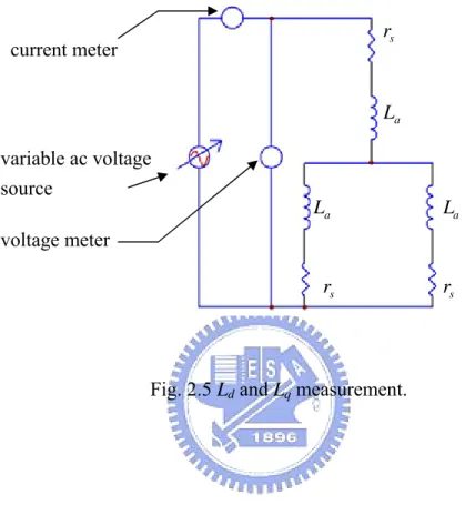
2.2. L

d

and L

q

measurement

The d-axis and q-axis inductance, Ld and Lq,of a PMSM in which the magnets are

buried in the rotor as shown in Fig. 2.3 can be measured with a single phase ac voltage source, see the connection below.

The applied voltage and current are recorded to calculate the inductance. The d-q axis inductance can be calculated as the equation shown below by varying the applied voltage from 0 to 100 volts approximately:

(2.19) where is is the measured current and vs is the measured voltage.

variable ac voltage source voltage meter current meter rs s r s r a L a L a L

Fig. 2.5 Ld and Lq measurement.

( )

2 2 3 2 1 60 2 1 or s s s q d vs ri i L L ⎟ − ⎠ ⎞ ⎜ ⎝ ⎛ = π

Chapter 3

Kalman Filter Estimator for A PMSM

y(k)

z

-1 ) ( ˆ k y

z

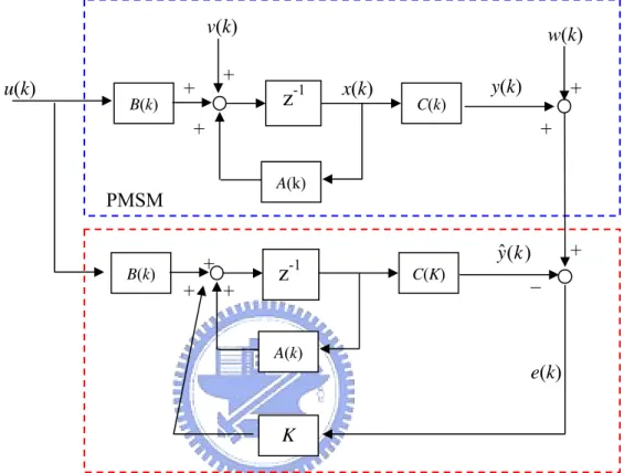
-1 + + + v(k) _w(k) K x(k) PMSM B(k) C(k) A(k) + + u(k) C(K) _{_} e(k) + + + + A(k) B(k)

Fig. 3.1 Structure of EKF.

Fig. 3.1 shows the basic block diagram of the extended Kalman filter (EKF) [9]. It shows that the EKF is based on the state equations of a PMSM. The upper block shows the PMSM state equations which looks like the lower block except the Kalman gain K and noise vectors v(k) and w(k). The actual output y(k) and estimated output y)(k)would be the same with the same input u(k) neglecting v(k) and w(k) which results e(k) to zero. In fact, this would not happen in reality and e(k) is not zero due to v(k) and w(k) which represent system and measurement noises respectively. In the experiment, u(k) and y(k) are voltage commands and motor phase currents decoupled on stationary frame respectively, see Fig. 1.2. The states

vector x(k) is defined as [ , iαs ,

β s

i θ , ω ] in which the unknown states, rotor position r θ r

and speed ω , are to be estimated according to the known currents and . The Kalman gain K will try to minimize e(k) to estimate the speeds and positions with the covariance matrices P, Q, R of the system state vector, system noise vector, and measurement noise vector respectively.

α s

i i_sβ

3.1. Kalman filter on rotor reference frame for a PMSM

β

q

r

ω

d

r

θ

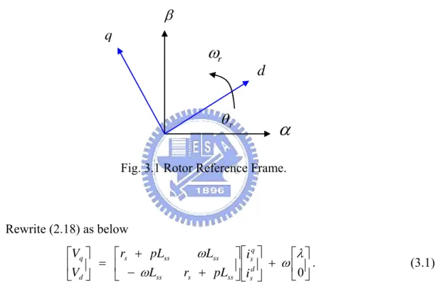
_α

Fig. 3.1 Rotor Reference Frame.

Rewrite (2.18) as below . (3.1) ⎥ ⎦ ⎤ ⎢ ⎣ ⎡ + ⎥ ⎦ ⎤ ⎢ ⎣ ⎡ ⎥ ⎦ ⎤ ⎢ ⎣ ⎡ + − + = ⎥ ⎦ ⎤ ⎢ ⎣ ⎡ 0 λ ω ω ω d s q s ss s ss ss ss s d q i i pL r L L pL r V V

The equation above is derived from an arbitrary d-q reference frame. To apply EKF algorithm, (3.1) needs to be present in differential equations which the state variables should be defined first. Let the state variables be , where and are stator current projecting to arbitrary d-q frame, t q s d s i i x=[ ω_rθ_r] d s i q s i r

ω is rotor rotation speed and θ is rotor angle referring to α axis r

fixed on stator “a” (as) axis. The output is , where and are the stator current referring to

t

i i

y=[_{α β}] i_α i_β

αβ reference frame. The input is , where and

are stator input voltage referring to

t p u V V u=[ _{α β} ] V_α V_β

αβ reference frame and up = ωλ.

There are two different coordinates, d-q and αβ frames. It’s also necessary to know the relation between these two frames:

. (3.2) ⎥ ⎦ ⎤ ⎢ ⎣ ⎡ ⎥ ⎦ ⎤ ⎢ ⎣ ⎡ − = ⎥ ⎦ ⎤ ⎢ ⎣ ⎡ β α θ θ θ θ r r r r q d cos sin sin cos

State equation forms:

Bu Ax x dt d _{= +} , Cx y= . (3.3)

Represent (3.1) in state equations:

⎥ ⎥ ⎥ ⎥ ⎥ ⎦ ⎤ ⎢ ⎢ ⎢ ⎢ ⎢ ⎣ ⎡ = r r q s d s i i x θ ω , _⎥⎥, . (3.4) ⎥ ⎦ ⎤ ⎢ ⎢ ⎢ ⎣ ⎡ = p u V V u _β α ⎥ ⎦ ⎤ ⎢ ⎣ ⎡ = β α i i y q s s r d s s d s s d i Li dt d L i r V = + −ω , s d q s r d s s s d s L V i i L r i dt d + + − = ω , (3.5) λ ω ω d _r s s r q s s q s s q i Li dt d L i r V = + + + , s q s p q s s s d s r q s L V L u i L r i i dt d _{=−ω − − +} , (3.6) where up=ωrλ. ⎥ ⎥ ⎥ ⎦ ⎤ ⎢ ⎢ ⎢ ⎣ ⎡ ⎥ ⎥ ⎥ ⎥ ⎥ ⎥ ⎥ ⎦ ⎤ ⎢ ⎢ ⎢ ⎢ ⎢ ⎢ ⎢ ⎣ ⎡ + ⎥ ⎥ ⎥ ⎥ ⎥ ⎦ ⎤ ⎢ ⎢ ⎢ ⎢ ⎢ ⎣ ⎡ ⎥ ⎥ ⎥ ⎥ ⎥ ⎥ ⎥ ⎦ ⎤ ⎢ ⎢ ⎢ ⎢ ⎢ ⎢ ⎢ ⎣ ⎡ − − − = ⎥ ⎥ ⎥ ⎥ ⎥ ⎦ ⎤ ⎢ ⎢ ⎢ ⎢ ⎢ ⎣ ⎡ p q d s s r r q s d s s s r r s s r r q s d s u V V L L i i L r L r i i dt d 0 0 0 0 0 0 0 1 0 0 0 1 0 1 0 0 0 0 0 0 0 0 0 0 θ ω ω ω θ ω . (3.7)

Rewriting the differential equations (3.5) and (3.6) in the form

Bu Ax x dt d + = ,

Cx y= .

and applying (3.2) in (3.7) yields

⎥ ⎥ ⎥ ⎦ ⎤ ⎢ ⎢ ⎢ ⎣ ⎡ ⎥ ⎥ ⎥ ⎥ ⎥ ⎥ ⎥ ⎦ ⎤ ⎢ ⎢ ⎢ ⎢ ⎢ ⎢ ⎢ ⎣ ⎡ − − + ⎥ ⎥ ⎥ ⎥ ⎥ ⎦ ⎤ ⎢ ⎢ ⎢ ⎢ ⎢ ⎣ ⎡ ⎥ ⎥ ⎥ ⎥ ⎥ ⎥ ⎥ ⎦ ⎤ ⎢ ⎢ ⎢ ⎢ ⎢ ⎢ ⎢ ⎣ ⎡ − − − = ⎥ ⎥ ⎥ ⎥ ⎥ ⎦ ⎤ ⎢ ⎢ ⎢ ⎢ ⎢ ⎣ ⎡ p s s r r r s r r r q s d s s s r r s s r r q s d s u V V L L L i i L r L r i i dt d β α θ θ θ θ θ ω ω ω θ ω 0 0 0 0 0 0 1 cos sin 0 sin cos 0 1 0 0 0 0 0 0 0 0 0 0 . (3.8)

The output equation is

. (3.9) ⎥ ⎥ ⎥ ⎥ ⎥ ⎦ ⎤ ⎢ ⎢ ⎢ ⎢ ⎢ ⎣ ⎡ ⎥ ⎦ ⎤ ⎢ ⎣ ⎡ − = ⎥ ⎦ ⎤ ⎢ ⎣ ⎡ r r q s d s r r r r i i i i θ ω θ θ θ θ β α 0 0 cos sin 0 0 sin cos

Now the complete state equations are

⎥ ⎥ ⎥ ⎥ ⎥ ⎥ ⎥ ⎦ ⎤ ⎢ ⎢ ⎢ ⎢ ⎢ ⎢ ⎢ ⎣ ⎡ − − − = 0 1 0 0 0 0 0 0 0 0 0 0 s s r r s s L r L r A ω ω , (3.10) ⎥ ⎥ ⎥ ⎥ ⎥ ⎥ ⎥ ⎦ ⎤ ⎢ ⎢ ⎢ ⎢ ⎢ ⎢ ⎢ ⎣ ⎡ − − = 0 0 0 0 0 0 1 cos sin 0 sin cos s s r r s r L L L B θ θ θ θ , (3.11) and _⎥. (3.12) ⎦ ⎤ ⎢ ⎣ ⎡ − = 0 0 cos sin 0 0 sin cos r r r r C θ θ θ θ

3.2. Kalman filter on stator reference frame for a PMSM

β

q

r

ω

d

r θ

α

Fig. 3.2 Stator Reference Frame.

In the arbitrary rotating frame, as shown in Fig. 2.1, θ is set to 90 electrical degrees to get a fixed coordinate αβ frame. Axis q and axis d are rotor quadrant and direct axes respectively. The (2.5) is presented below for quick reference ,

0 0 0 0 0 0 0 0 0 0 2 3 0 2 3 0 3 2 qd s qd s qd s qd s qd s p r i V + + ⎥ ⎥ ⎥ ⎥ ⎥ ⎥ ⎦ ⎤ ⎢ ⎢ ⎢ ⎢ ⎢ ⎢ ⎣ ⎡ − = ω λ λ (3.13)

where ω would be 0 in the fixed coordinate. Then (3.13) becomes

, (3.14) 0 0 0 0 βα βα βα βα _λ s s s s p r i V = +

(

)

( )

(

abc

)

r abc sr abc s abc s abc s abc s abc s abc s s pT pT Tp Tp T p L i L i pλβα0 = λ = λ + λ = λ = + , (3.15)

. (3.16) βα βα s abc s s abc s abc s abc s i TL T i L i TL = −1 =

In (2.12), we replace qd with βα , it becomes

(

)

βα r sr sr abc r abc sr L i L i L T 0 0 0 0 2 3 0 0 0 2 3 ⎥ ⎥ ⎥ ⎥ ⎥ ⎥ ⎦ ⎤ ⎢ ⎢ ⎢ ⎢ ⎢ ⎢ ⎣ ⎡ = , (3.17) ⎥ ⎦ ⎤ ⎢ ⎣ ⎡ ⎥ ⎦ ⎤ ⎢ ⎣ ⎡ − ⎥ ⎥ ⎥ ⎦ ⎤ ⎢ ⎢ ⎢ ⎣ ⎡ = ⎥ ⎦ ⎤ ⎢ ⎣ ⎡ d r q r r r r r sr sr sr sr i i L L θ θ θ θ λ λ α β cos sin sin cos 2 3 0 0 2 3 . (3.18)

For a PMSM, we set q to 0, then (3.18) yields

r i ⎥ ⎥ ⎥ ⎦ ⎤ ⎢ ⎢ ⎢ ⎣ ⎡ = ⎥ ⎦ ⎤ ⎢ ⎣ ⎡ ⎥ ⎥ ⎥ ⎦ ⎤ ⎢ ⎢ ⎢ ⎣ ⎡ − d r r sr d r r sr d r q r r sr r sr r sr r sr i L i L i i L L L L θ θ θ θ θ θ cos 2 3 sin 2 3 cos 2 3 sin 2 3 sin 2 3 cos 2 3 . (3.19) Rewrite (3.14), we get βα βα βα βα θ θ ω s abc s d r r sr d r r sr r s s s i dt d L i L i L i r V + ⎥ ⎥ ⎥ ⎦ ⎤ ⎢ ⎢ ⎢ ⎣ ⎡ − + = sin 2 3 cos 2 3 . (3.20)

In (3.20), the ωrterm comes from the differentiation of (3.19)

Represent（3.20）as below, , (3.21) r r s s s s s r i L i Vβ = β + β + ω λ cosθ . (3.22) r r s s s s s r i L i Vα = α + α − ω λ sinθ

Transfer (3.21) and (3.22) into state equation form:

s s r r s s s s s L V L i L r i dt d _{β β} λ_{ω θ} β + − − = cos , (3.23)

s s r r s s s s s L V L i L r i dt d _{α α} λ_{ω θ} α + + − = sin . (3.24)

Another differential equation form, x f_{( )}x Bu dt

d

+

= , is introduced with state vector

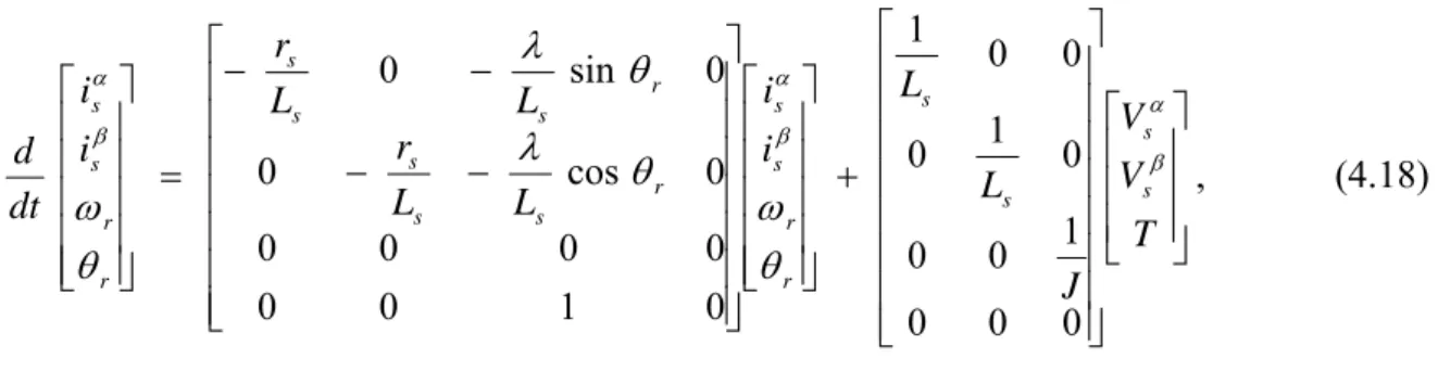
, input and output state variables , then the complete state equations are

t s s i i x=[α β ω_rθ_r] u=[V_αV_β]t y=[i_sα i_sβ]t

( )

⎥ ⎥ ⎥ ⎥ ⎥ ⎥ ⎥ ⎦ ⎤ ⎢ ⎢ ⎢ ⎢ ⎢ ⎢ ⎢ ⎣ ⎡ − − + − = r r r s s s s r r s s s s L i L r L i L r x f ω θ ω λ θ ω λ β α 0 cos sin , (3.25) ⎥ ⎥ ⎥ ⎥ ⎥ ⎥ ⎥ ⎦ ⎤ ⎢ ⎢ ⎢ ⎢ ⎢ ⎢ ⎢ ⎣ ⎡ = 0 0 0 0 1 0 0 1 s s L L B , (3.26) and . _⎥ (3.27) ⎦ ⎤ ⎢ ⎣ ⎡ = 0 0 1 0 0 0 0 1 C

3.3. Selection of the time-domain machine model

Comparing (3.10), (3.11), and (3.12) with (3.25), (3.26), and (3.27) we can observe some differences. It is possible to have EKF implementations using time-domain machine models expressed in the stationary or rotor reference frame. Obviously the selection of the reference frame has a great effect for the execution time in real time implementation using a DSP. In (3.26) and (3.27), the elements of these matrices are constants which can make coding easier and reduce calculation time needed, especially in view of the computational intensity of the EKF.

As discussed above, the EKF model would be based on (3.25), (3.26) and (3.27) derived from the stationary frame for the purpose of faster calculation.

Chapter 4

Simulations of EKF

The Matlab/simulink has been used throughout all the analysis, design and simulations. It’s easier to simulate the EKF using Matlab language files (M files) instead of transfer functions in Matlab/simulink. Besides, the advantage of the M file is that it is easily converted into an assembly program. So the PMSM models of stator reference frame are adopted for the S-function and so are the EKF models.

As mentioned in section 3.2, the state vector, , have to be estimated. The input is defined as and the output vector is . The state variables form of the equations will be obtained by assuming that the rotor inertia has an infinite value (thus the derivative of the rotor speed is negligible compared with the other system variables, and any mechanical load parameter, as well as the load torque,

t s s i i x=[ α βω_rθ_r] t V V u=[ _{α β}] t s s i i y=[ α β] 0 / dt = dω_r ) and dt d r r θ /

ω = . Although in practice the rotor inertia is not infinite, the required correction is performed by the Kalman filter algorithm. Thus the following state-variable equation is obtained:

( )

x Bu f x dt d _{= + (4.1)}

and the output vector is

Cx

y = . (4.2)

In section 3.2., f(x) is defined as:

( )

⎥ ⎥ ⎥ ⎥ ⎥ ⎥ ⎥ ⎦ ⎤ ⎢ ⎢ ⎢ ⎢ ⎢ ⎢ ⎢ ⎣ ⎡ − − + − = r r r s s s s r r s s s s L i L r L i L r x f ω θ ω λ θ ω λ β α 0 cos sin . (4.3)

⎥ ⎥ ⎥ ⎥ ⎥ ⎥ ⎥ ⎦ ⎤ ⎢ ⎢ ⎢ ⎢ ⎢ ⎢ ⎢ ⎣ ⎡ = 0 0 0 0 1 0 0 1 s s L L B (4.4)

and the output transformation matrix is

. (4.5) ⎥ ⎦ ⎤ ⎢ ⎣ ⎡ = 0 0 1 0 0 0 0 1 C

As mentioned in section 3.3, in contrast to the transformation matrix of the model expressed in the rotor reference frame, see (3.10), the matrix as shown in (4.4) and (4.5) contains only constant elements, and it results in simplifications in the implementation of the EKF. The system described by (4.3) is a non-linear system. It is this non-linearity which ensures that the EKF has to be used, and not the conventional, linearized Kalman filter. It should be noted that the time-discrete model is now put into the following form where the noise vectors have also been added to obtain a system model required by the EKF:

) ( ) ( ) ( ] ), ( [ ) (k f x k k B k u k v k x = + + , (4.6) ) ( ) ( ) ( ) (k C k x k w k y = + . (4.7)

The covariance matrices can be chosen to be diagonal, and Q is a 4 by 4 matrix, R is a 2 by 2 matrix, and P0=P(0) is a 4 by 4 matrix. In general they are assumed to take the form

, (4.8) ) ) ) ( 0 diag a,a,b,c Q Q= = , (4.9) ( 0 diag e,e,f,g P = and R=R₀ =diag(m,n . (4.10)

The motor behavior with real position feedback and the EKF will be illustrated in simulation and experiments.

4.1. The steps of the discretized EKF algorithm on stator

reference frame

The steps of the discretized EKF algorithm are as follows:

Step 1: Initialization of the state vector and covariance matrices

The initial values of the state vector x0=x(t0) and noise covariance matrices Q0 and R0

are set, together with the starting value of the state covariance matrix P0. It is important to

note that in general, if incorrect initial values are used, the EKF algorithm will not converge to the correct values. For the initial position of the PMSM, θ_r, which can be obtained using the method of aligning the rotor by applying stator current at “as” axis, then the rotor will be aligned at “as” (or α ) axis. For a brushless DC motor, the rotor initial position can be obtained by examining the stator currents applied by a certain duty cycle of the output phase voltages, this method will be discussed in detail in chapter 4.

Step 2: Prediction of the state vector

Prediction of the state vector at sampling time (k+1) from the input u(k), the state vector at previous sampling time x(k), by using f and B, is obtained by performing

] [ ] [ ) ( ) 1 ( ) 1 (k |k x k x k | k T f (k | k) Bu(k) x(k) T f (k) Bu(k) x + = + = + x + = + x + . (4.11)

On the right side equation, the simplified notation has been used, and a simple rectangular integration technique is used by using the previous state estimate x(k|k), and also the mean voltage vector u(k) which is applied to the motor in the period t_kto t_k+1.

Step 3: Covariance estimation of prediction The covariance matrix of prediction is estimated as

Q k F | k k P | k k F(k)P T k | k P | k k P( +1 )= ( )+ [ ( +1 +1)+ ( +1 +1) T( )]+ , (4.12)

where F is the gradient matrix:

x f(x) k F ∂ ∂ = ) ( , (4.13) ⎥ ⎥ ⎥ ⎥ ⎥ ⎥ ⎥ ⎦ ⎤ ⎢ ⎢ ⎢ ⎢ ⎢ ⎢ ⎢ ⎣ ⎡ − − − = 0 1 0 0 0 0 0 0 sin cos 0 cos sin 0 r s r s s s r s r s s s L L L r L L L r θ ωλ θ λ θ ωλ θ λ . (4.14)

Step 4: Kalman filter gain computation

. (4.15) 1 ] ) 1 ( [ ) 1 ( ) 1 ( T T -R C |k k CP C |k k P k K + = + + +

Step 5: State vector estimation

The state vector estimation at time (k+1) is performed through the feedback correction scheme, which makes use of the actual measured quantities (y):

xˆ(k+1|k)=x(k+1|k)+k(k+1)[y(k+1)-Cx(k+1|k)]. (4.16)

Step 6: Covariance matrix of estimation error

. (4.17) ) 1 ( ) 1 ( ) 1 ( ) 1 1 ( ˆ _{k |k P k |k -K k CP k |k} P + + = + + +

Step 7: k=k+1, x(k)=x(k-1), P(k)=P(k-1) and go to Step 1.

It should be noted that this scheme requires the measurement of the stator voltages and currents. In a PWM voltage-source inverter, it is possible to reconstruct the stator voltage according to the DC bus voltage and switching states of the power switches. If so, we need a voltage sensor to detect the DC bus voltage and connect it to A/D interface of the DSP. As we know, PWM type inverter can be a noisy source which means you will pick up noises when you measure the motor phase voltages. To avoid the noises, using some filtering is necessary

but it will lead to another problem, phase lag, and this would cause some inaccuracies and convergence problem during the calculations of EKF algorithm. Another possible way is to use stator voltage references instead of the real phase voltages, thus we can get rid of the voltage sensor and simply the software and hardware.

4.2. Matlab/simulink simulation of the EKF

Fig. 4.1 PMSM with EKF simulink model.

4.2.1. Description of the function blocks

In Fig. 4.1, the descriptions of the blocks are as below:

dq2abc: Transform d-q current references to abc current references.

INPUT:

¾ iqref: q-axis current reference coming from PI speed regulator. ¾ idref: d-axis current reference, set to 0.

¾ ioref: Set to 0.

¾ thetae: Rotor position, it is needed for coordinates transformation. OUTPUT:

¾ iabcr: Motor three phase current references. PWM inv 2: Current regulator.

¾ iref: Three phase currents reference input.

¾ iabc: Three phase currents feedback coming from the motor. OUTPUT:

¾ va,vb,vc: Motor three phase voltages.

Stator reference: Motor model in stator reference (alpha-beta),which is based on s functions. INPUT:

¾ va,vb,vc: Motor three phase voltages input.

¾ Friction: Friction input coming from mechanical parts like bearings and loads. OUTPUT:

¾ iabc: Motor three phase current outputs which can be used as monitor and feedback. ¾ w_e: Motor speed in electric degrees.

¾ theta_e: Rotor position in electric degrees. ¾ Te: Motor output torque.

EKM: Extended Kalman filter model. INPUT :

¾ va,vb,vc: The inputs comes from the motor phase voltages. ¾ ia,ib,ic: The inputs comes from the motor phase currents. OUTPUT：

¾ i_alpha_e: Estimated alpha axis current output from EKM. ¾ i_beta_e: Estimated beta axis current output from EKM. ¾ w_e: Estimated rotor speed in electric degrees from EKM. ¾ theta_e: Estimated rotor position in electric degrees from EKM. ¾ torque_es: Estimated torque from EKM.

4.2.2. Description of the motor simulink model in stator reference frame

Fig. 4.2 A PMSM Simulink model in stator reference frame.

Fig. 4.2 shows the block diagram of PMSM in stator reference frame. The inputs are the motor three phase voltages like the real motor. The outputs are three phase currents, motor speed and rotor position. It’s easy to simulate motor behavior using matrix Matlab/simulink S function. According to (3.23) and (3.24), the state equations for simulation in S function is shown below: ⎥ ⎥ ⎥ ⎦ ⎤ ⎢ ⎢ ⎢ ⎣ ⎡ ⎥ ⎥ ⎥ ⎥ ⎥ ⎥ ⎥ ⎥ ⎦ ⎤ ⎢ ⎢ ⎢ ⎢ ⎢ ⎢ ⎢ ⎢ ⎣ ⎡ + ⎥ ⎥ ⎥ ⎥ ⎥ ⎦ ⎤ ⎢ ⎢ ⎢ ⎢ ⎢ ⎣ ⎡ ⎥ ⎥ ⎥ ⎥ ⎥ ⎥ ⎥ ⎦ ⎤ ⎢ ⎢ ⎢ ⎢ ⎢ ⎢ ⎢ ⎣ ⎡ − − − − = ⎥ ⎥ ⎥ ⎥ ⎥ ⎦ ⎤ ⎢ ⎢ ⎢ ⎢ ⎢ ⎣ ⎡ T V V J L L i i L L r L L r i i dt d s s s s r r s s r s s s r s s s r r s s β α β α β α θ ω θ λ θ λ θ ω 0 0 0 1 0 0 0 1 0 0 0 1 0 1 0 0 0 0 0 0 0 cos 0 0 sin 0 , (4.18)

where T means torque, is the system inertia. The output torque equation is presented as below:

) ) ( ( 5 . 1 q s d s q d q s L L i i i P T = λ + − . (4.19)

The motor model is based in the stator reference frame, so we need to convert and to and . The transfer matrix:

α s i isβ d s i isq ⎥ ⎦ ⎤ ⎢ ⎣ ⎡ ⎥ ⎦ ⎤ ⎢ ⎣ ⎡ − = ⎥ ⎦ ⎤ ⎢ ⎣ ⎡ β α θ θ θ θ r r r r q d cos sin sin cos . (4.20) Apply (4.20) to (4.19), it yields ) sin cos )( ( ) cos sin ( ( 5 . 1 P i_{s r} i_{s r} L_d L_q i_{s r} i_{s r} T = λ −α θ + β θ + − α θ + β θ (−i_sαsinθ_r +i_sβcosθ_r)). (4.21) The equation (4.21) will be used to calculate the output torque in the simulation. The output states variables: ⎥ ⎥ ⎥ ⎥ ⎥ ⎦ ⎤ ⎢ ⎢ ⎢ ⎢ ⎢ ⎣ ⎡ ⎥ ⎥ ⎥ ⎥ ⎦ ⎤ ⎢ ⎢ ⎢ ⎢ ⎣ ⎡ = r r s s i i y θ ω β α 1 0 0 0 0 1 0 0 0 0 1 0 0 0 0 1 . (4.22)

We will use (4.18) and (4.22) in the file pmstator.m

pmstator1.m file

%%%%%%%%%%%%%%%%%%%%%%%%%%%%%%%%%%%%%%% % Motor model in stator reference frame

%%%%%%%%%%%%%%%%%%%%%%%%%%%%%%%%%%%%%%% function [sys,x0,str,ts]=pmstator(t,x,u,flag); Rs=5; Ld=10e-3; Lq=10e-3; Fm=0.175; J=0.8e-3; C=[1 0 0 0; 0 1 0 0; 0 0 1 0; 0 0 0 1]; switch flag case 0, sizes=simsizes;

sizes.NumDiscStates=0; sizes.NumOutputs=4; sizes.NumInputs=4; sizes.DirFeedthrough=0; sizes.NumSampleTimes=1; str=[]; ts=[0 0]; x0=[0; 0; 0; 0]; sys =simsizes(sizes); case 1, U=[u(1);u(2);u(3)]; A=[-Rs/Ld 0 Fm/Ld*sin(x(4)) 0; 0 -Rs/Lq -Fm/Lq*cos(x(4)) 0; 0 0 0 0; 0 0 1 0]; B=[ 1/Ld 0 0; 0 1/Lq 0; 0 0 1/(J+u(4)); 0 0 0 ]; sys=A*x+B*U; case 3, sys=C*x; case 4, sys=[]; case 9, sys=[]; end

4.2.3. Description of the EKF simulink model in stator reference frame

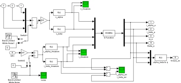
Fig. 4.3 The EKF model on stator reference frame.

Examining Fig. 4.3 finds the structure is quite similar to the model in Fig. 4.2, the input v_alpha, v_beta and the output i_aplha, i_beta, w_e, theta are the same with Fig. 4.2. The major differences are EKF needs currents feedback to calculate Kalman gain and there are white noises inputs injected to the voltages v_alpha, v_beta and currents i_alpha, i_beta. The white noise is appeared as Fig. 4.4.

According to section 3.1, we can compose Matlab language as below: EKM6a.m file

function [sys,x0,str,ts]=EKM6a(t,x,u,flag,P,Q,R); %global Rs Ld Lq Fm v_alpha v_beta i_alpha i_beta; %global P Q R fid;

%global out fit; Rs=5; Ld=10e-3; Lq=10e-3; Fm=0.175; T=5e-4; %i=0; Bd=[1/Ld 0; 0 1/Lq; 0 0; 0 0]; H=[1 0 0 0; 0 1 0 0]; switch flag case 0, %ekmini; sizes=simsizes; sizes.NumContStates=0; sizes.NumDiscStates=4; sizes.NumOutputs=4; sizes.NumInputs=4; sizes.DirFeedthrough=0; sizes.NumSampleTimes=1; str=[]; ts=[0.0005 0]; x0=[0; 0; 0; 0]; sys = simsizes(sizes); case 2,

% Step 1:Initialization of the state vector and covariance matrices

Uk=[u(1);u(2)]; Y=[u(3);u(4)];

% Step 2:Prediction of the state vector

fx=[-Rs/Ld*x(1)+Fm/Ld*x(3)*sin(x(4)) ; -Rs/Lq*x(2)-Fm/Lq*x(3)*cos(x(4)) ;

0 ; x(3) ]; F=[-Rs/Ld 0 Fm/Ld*sin(x(4)) Fm/Ld*x(3)*cos(x(4)); 0 -Rs/Lq -Fm/Lq*cos(x(4)) Fm/Lq*x(3)*sin(x(4)); 0 0 0 0; 0 0 1 0]; x1=x+T*(fx+Bd*Uk);

% Step 3: Covariance estimation of prediction

P1=P+T*(F*P+P*F')+Q; % P1 is 4x4 % Step 4: Kalman filter gain computation

K1=P1*H'*inv(H*P1*H'+R);% K1 is 4x2 % Step 5: State vector estimation

h=[x1(1);x1(2)]; sys=x1+K1*(Y-h);

% Step 6: Covariance matrix of estimation error P=P1-K1*H*P1; case 3, sys=x; case 4, sys=(round(t/T)+1)*T; %sys=[]; case 9, sys=[]; end