行政院國家科學委員會補助專題研究計畫成果報告
※※※※※※※※※※※※※※※※※※※※※※※※※
※
※
※
備兌型認購權證的價格發現功能
※
※
※
※※※※※※※※※※※※※※※※※※※※※※※※※
計畫類別:□個別型計畫
□整合型計畫
計畫編號:NSC 89-2416-H-004-083
執行期間:89 年 8 月 1 日至 90 年 7 月 31 日
計畫主持人:周行一
國立政治大學財務管理系教授
計畫參與人員:陳麗雯
國立政治大學財務管理系博士班研究生
本成果報告包括以下應繳交之附件:
□赴國外出差或研習心得報告一份
□赴大陸地區出差或研習心得報告一份
□出席國際學術會議心得報告及發表之論文各一份
□國際合作研究計畫國外研究報告書一份
執行單位:國立政治大學財務管理系
中
華
民
國
90 年
10 月
30 日
行政院國家科學委員會專題研究計畫成果報告
計畫編號:NSC 89-2416-H-004-083
執行期限:89 年 8 月 1 日至 90 年 7 月 31 日
主持人:周行一 國立政治大學財務管理系教授
計畫參與人員:陳麗雯
國立政治大學財務管理系博士班研究生 一、中文摘要 本論文探討認購權證發行券商的次級 市場交易行為,本文的特殊資料庫讓本文 有機會探討這個過去無法研究的問題,本 文發現發行券商是認購權證次級市場的主 要流動性供給者,也對標的股票的流動性 有重要的幫助。發行券商的交易行為比較 像搶帽者,而非部位交易者或指定造市 者。發行券商的主要獲利來源為發行期間 收取的權利金,但是在次級市場的交易卻 賠錢,因此,雖然一般人認為發行券商收 取的權利金過高,但是卻可增加券商在次 級市場提供流動性的意願。本文亦發現勸 商的次級市場交易對權證及標的股票的價 格有顯著的影響。 關鍵詞:認購權證、交易行為、流動性、 搶帽者 AbstractThis paper studies the trading behavior of derivative warrant issuers on the Taiwan Stock Exchange. We use a unique dataset that allows us to explore this issue. The issuers are the major liquidity providers on the warrant market. In addition, the issue of warrant also helps increase the liquidity of the underlying. The issuers trade mainly like scalpers rather than position traders or designated market makers. The premium the warrant issuers collect before the start of secondary market trading is the main source of their profits. In general, they lose money from trading on the secondary market. Our finding provides a new insight on the regulation of market maker’s (underwriter’s) profit. If we allow liquidity providers to
charge a high price for their services, the market liquidity could enhance. The trading of the warrant issuers have significant impacts on the price of warrants and the underlying.
Keywords: derivative warrant, trading behavior, liquidity, scalper 二、緣由與目的
Derivative warrants are common in Asia and Europe and sometimes more popular than stock options.1 Derivative warrants and options are identical in terms of their contractual characteristics. However, their trading mechanisms are quite different. Derivative warrants are traded like stocks with limited supply set by the issuer. So the outstanding amount of derivative warrants is fixed. Thus, it is not possible to sell warrants without already having warrants in hands. In addition, since the derivative warrants are issued by investment banks that are not the issuers of the underlying stocks, the issuers are the only party that is obligated to deliver in the event of warrant exercise. ____________________________________
1
In Hong Kong, Singapore, Australia, Taiwan, and Germany derivative warrants are heavily traded. In Hong Kong
derivative warrants are actually more liquid than options with the same underlying (Duan and Yang (1999)). In Taiwan, derivative warrants are quite liquid as well (See Chow, Lee, Lee, Liu and Chen, (2000)).
Derivative warrants are usually issued by investment banks for the purpose of making trading and issuing profits. The underlying stocks of the derivative warrants are not the stocks of the issuers. In contrast, equity warrants, which are common in the US, are issued by the firms of the underlying stocks for financing purpose.
Hence, in order to lock in profits or to reduce risk the issuers may have incentives to buy warrants to reduce the number of outstanding warrants.
In contrast, the open interest of options is in principle unlimited. Traders can short and long options without a position in hands. In addition, market makers of options
presumably have better profit prospects when open interest is high, not to mention that they cannot directly influence the size of open interest. Because of these reasons, it is conceivable that warrants traders could behave quite differently from options traders. To our knowledge all major options exchanges around the world have designated market makers. But there are no designated market makers on warrants markets.
Although the issuer of derivative warrants is the presumed market maker, they could conceivably behave quite differently from an options market maker for several reasons. Firstly, if the issuer of warrants makes the market, it is out of its interest in maintaining a market that has potential for future issues. The options market maker makes market to earn short-term trading profits. Secondly, the options market maker usually has to keep a constant presence on the market by posting two-way quotes, but the warrants issuer does not have to. The warrants issuer supplies liquidity by submitting limit orders like other traders would. Thirdly, when the issuer buys the warrants, the outstanding number of warrants is reduced. However, the open position of options is not necessarily affected by the trading of options market maker. Fourthly, the warrants issuer can reduce its risk by buying warrants, i.e., reducing the outstanding amount of warrants, but the options market maker needs to keep a
minimum presence on the market as required by the exchange. Fifthly, the warrants issuer has to “market” its warrants, while the option market maker does not have to. To the extent that the subscribers of warrants are the customers of the issuer the relationship between the issuer and the investors is different from that between options market makers and public traders.
This paper is the first attempt in the literature to study the trading behavior of
warrant issuer. The study is interesting in several aspects. One, since derivative warrants are popular in many markets, studying the trading behavior of warrant issuer will give clue to the design of trading mechanism that fosters the growth of warrant market.
Two, much has been done on the effects the listing or trading of options on the
underlying market.2 But very little is done on the same issue with respect to warrants.3 Our analysis would help the general
understanding of the mechanism through which the trading of warrants affects the performance of the underlying asset. Furthermore, our analysis is more detailed than existing work. We use the
trade-by-trade data of all the warrant traders to analyze the dynamics of the trading of warrant issuer and its impacts on the underlying and the warrant market. Our approach is somewhat similar to Berkman (1996) that analyzes the price behavior of stocks and options around large option trades. He finds that after market makers trade the option quotes tend to return to their pretrade level and there is a weak temporary effect on the stock price. This finding is consistent with the hypothesis that inventory control by market makers spills over to the stock exchange.
Three, in academic literature as well as in financial practice the pricing of warrants are often treated as very similar to options. But pricing model error could have profound ____________________________________
2 Chan, Chung and Johnson (1995) find different intraday patterns of bid-ask spreads for actively traded CBOE options and for their NYSE-traded underlying stocks. Fedenia and Gramatikos (1992) show that options listing significantly affects the spreads on the underlying stocks. Gjerde and Saettem (1995) show that on the Norwegian markets option listing is associated with a temporary price increase on the introduction day and a substantial decline in the bid-ask spreads of the underlying stocks. There are quite a few other studies on the impacts of the introduction of options on the price of the underlying stocks. See, e.g., Trenepohl and Dukes (1979), Klemkosky and Maness (1980), Conrad (1989), Gemmill (1989), Skinner (1989), Detemple and Jorion (1990), Damodaran and Lim (1991), and Chamberlain, Cheung, and Kwan (1993).
3 Alkeback and Hagelin (1998) find that the introduction of equity warrants has no effect on the price of they underlying stocks.
impact on the risk management of the warrant issuer and the trading efficiency of market participants. Some recent studies address the microstructure issue that affects the pricing of options. Jameson and Wilhelm (1992) show that risks associated with the inability to rebalance an option position continuously and uncertainty about the return volatility of the underlying stock each account for a statistically and
economically significant proportion of the bid-ask spreads quoted for a sample of Chicago Board Options Exchange options. They suggest that the risks may influence the theoretical bounds on option prices.
Figlewski (1998) reviews several sources of model risk facing derivatives traders. There is the risk that a given model may be misspecified with respect to the return distribution of the underlying asset, which could lead to mispricing and expose traders to unknown, excessive risk due to incorrect risk management based on the incorrect model. Green and Figlewski (1999) analyze to what extent the damage due to model risk can be limited by pricing options using a higher volatility than the best estimate from historical data.4
Brenner, Eldor and Hauser (2001) find that illiquidity (on the options market) affects the value of currency options. Nontradable options issued by the Central Bank of Israel are priced about 21% less than the exchange traded options listed on the Tel-Aviv Stock Exchange. The reason is that the central bank options can be replicated by the
exchange-traded options only at a substantial transaction cost. On the TSEC warrants tend to have different underlying stocks. The warrant issuer is the only market maker and the writer of the warrant that, according to our finding, constitutes about 20% of the trading. Since the issuer can significantly affect the liquidity of the warrant, it is important to understand how the warrant issuer trades. If warrants issuers behave ____________________________________
4 The warrants issuers in Taiwan adopt exactly this type of strategy by setting the issue price of warrants to have implied volatility higher than the observed historical volatility.
differently from options market makers, an analysis of how the trading of warrants issuers affects the prices of warrants and the underlying assets can help researchers to incorporate theses microstructure issues in their research of the pricing of warrants. The remainder of the paper is organized as follows. Section I introduces the market mechanism of the primary and secondary market of the Taiwan Stock Exchange
(TSEC). Section II explains the
characteristics and the handling of our data. Testable hypotheses and testing methodology are discussed in Section III. We present our empirical results in Section IV. Section V concludes the paper.
三、結果與討論
I. Mar ket Micr o-Str uctur e of Der ivative War r ants and Their Under lying Stocks on
the TSEC
A. The Primary Market of Warrants
Derivative warrants have been traded on the TSEC since September of 1997. All the warrants on the TSEC are issued by securities firms. One unit of warrant is exercised for one underlying share. Warrants on the same underlying stock can be issued more than once by the same issuer and/or different issuers. But the total number of outstanding warrants cannot exceed 20% of the amount of outstanding shares of the underlying stock. The market value of any issue has to be no less than NT$ 200 millions. The issuer has to apply for the approval of the Securities and Futures Commission (SFC) to issue new warrants. Afterwards it usually takes more than 10 days for the issuer to place the warrants to interested buyers. The issuer is allowed to keep as much as 20% of the whole issue as inventory for the purpose of making the market for the warrants. Since more than 80% of the issue has to be purchased by investors for it to be considered by the SFC as qualified for secondary market trading, sometimes the issuer has to recruit
involuntary buyers by promising to buy back the warrants at a price the same as or higher than the issue price. That is the reason why in the first week of secondary market trading
the issuer sometimes buy back a large proportion of outstanding warrants. B. The Secondary Market
The trading mechanism for warrants and the underlying stocks on the TSEC are identical. So warrants are traded just like stocks. The TSEC is an electronic, order driven, call market without designated market makers. The market liquidity is provided by limit orders. Except for the proprietary traders of securities firms (dealers) who can submit orders directly to the TSEC, all traders must submit orders to the TSEC through their brokers. In terms of secondary market trading the warrant issuer has the same status as dealers.
The TSEC matches orders according to the price-time priority rules that conform to the trading mechanism of a call market. The TSEC relies on the call mechanism for determining transaction prices throughout the trading day. For the opening call between 8:30 and 9:00 A.M. orders can be submitted to the TSEC. At 9:00 A.M. the first call is conducted. After the open orders are matched about every 4 to 50 seconds throughout the trading day. Basically, in between two calls orders are sequentially accepted by the computer and matched to maximize the trading volume. If after a call a sufficient number of orders have entered the system so that a transaction price can be determined, the TSEC will conduct another call immediately. However, there can be only two back-to-back calls like this. So the duration of a call period can vary from few seconds to approximately 50 seconds. After the second all, the computer would wait for as long as 50 seconds to initiate another call, depending on the order flow.
After each call the transaction price, transaction volume, the highest bid price and the lowest ask price among unmatched orders are released to the public. At the close the exchange conducts the last call for each stock. Remaining orders after the last call are removed from the book.
The TSEC has a daily price limit of 7% for the underlying stocks. The price limit for the warrant is the actual dollar amount of the price limit for the stock. Suppose that an underlying stock closes at NT$ 100 on the
previous business day. Then the range of price change today is NT$ 14 (NT$ 7 up plus NT$ 7 down) for both the warrant and stock. Since the price of warrant is usually much lower than the stock, the actual price limit for the warrant is much less stringent than the stock. In addition, except for the open price that is allowed to reach the daily price limit, all subsequent trades on the underlying stocks are imposed an intraday two-tick price limit that mandates the transaction price to move within two ticks of the price
determined in the previous call. But warrants are not constrained by the two-tick limit.
Only limit orders are allowed on the TSEC. To secure matching priority, traders need to submit limit orders hitting the daily price limits (limit orders with prices beyond the price limits are not accepted by the computer). This type of price-limit orders can achieve the effect of market orders.5 For this reason, Taiwanese practitioners call these orders market orders. Thus, on the TSEC traders can aggressively submit market orders to enhance the probability of trade and yet have some price protection from the intraday price limit. Unless the previous transaction price is within two ticks of the daily price limit, market orders would not be matched at the daily price limit. Thus, traders who prefer trade immediacy would place market orders. However, dealers and warrant issuers can only submit limit orders, which puts the issuers at a disadvantageous position relative to other traders in securing execution immediacy.
Except for the transaction cost the warrant issuer does not have regulatory advantages over other traders. All the traders on the TSEC have the same access to the trade information and intraday news release. All traders are subject to a transaction tax of 3% of the transaction amount on the sell side only. However, the warrant issuer bears a lower transaction fee than non-dealer traders. The brokerage fee for buy and sell is 0.1425% on each side for ____________________________________
5
If market orders are allowed, according to Schwartz (1991), they are equivalent to limit orders written at the highest allowable call price for buy orders and the lowest allowable call price for sell orders.
non-dealer traders. For the issuer there is no brokerage fee. The transaction fee for the warrant issuer is 0.015% on each side of trade.
II. Data
We employ the data of warrants and their underlying stocks that are listed between September of 1997 and May of 1999. We only include the warrants that are listed and mature during the sample period. There are 14 plain vanilla warrants and 4 warrants for which the underlying asset is a portfolio of stocks (portfolio warrants). To focus on the trading behavior of the issuers of warrants that are more like exchange-traded stock options, we exclude the four portfolio warrants.
The major data set of our study is the tick-by-tick transaction data of the TSEC. Since the TSEC is completely automated, the transaction data are complete. The
transactions are recorded at the time when they occur in the system. Our data allow us to identify the issuer’s transaction and to trace his entire trading.
Table I reports the summary statistics of warrants and the underlying stocks. The table shows the name of the underlying stock, exercise price, the stock prices on the issue date and the listing date, the implied volatility, the estimated volatility for the year before the warrant is issued, the number of warrants issued as a percentage of the number of underlying shares outstanding, the listing date and the maturity date of the warrants.
III. Testable Hypotheses
A. The Trading Behavior of Warrant Issuers
On an option market like CBOE three types of traders make the market: scalpers, position traders and designated market makers.6 A scalper makes a two-sided ____________________________________
6 According to Mayhew (forthcoming) after 1987 CBOE started to list some options under a Designated Primary Marketmaker (DPM). In 1991 the Pacific Exchange began to assign options to a Lead Market Maker (LMM). The AMEX and PHLX trade options under a specialist structure resembling that used in
market by making bids and offers. The scalper trades frequently during the day hoping to make very short-term profits without carrying inventory overnight. They manage risk by shedding positions quickly even at a loss. As Najarian (1992, p. 9) puts it, “… .if the trader would not have
established the trade at the current prices, the trade would be eliminated, even if it meant taking a loss. In this way the scalpers would turn over their inventory on a more regular basis and thus, free capital for other trades.” So scalpers are short-term speculators.
Position traders, instead, are more like arbitragers. They tend to have greater capital base than scalpers, which allows them to establish and hold large positions. They search for disparities in option pricing and then create an arbitrage between one or more option classes and the underlying stock or futures contract. Their trading edge relies on their ability to manage the risk of their arbitrage positions. They do not aim to sell premium to make a quick profit.
Unlike scalpers and position traders who do not necessarily maintain the market at all times the designated market makers are required to maintain a two-sided market constantly. For the designated market maker the benefit of bearing the stringent market making responsibility is usually the guarantee of participation in the market, fee discount and reduction in the margin
requirement for writing options. For the designated market maker to make profits from the quoted spread he must be skillful in assembling a hedged position in the
underlying stock. Jameson and Wilhelm (1992) find that uncertainty about the return volatility of the underlying stock accounts for a significant portion of the bid-ask spreads of CBOE options.
The trading behavior of the three types of market makers exhibits distinct features. Since a scalper speculates on short-term option price movement without holding a hedged position in the underlying stock, he primarily trades on the options markets only. In addition, the trades are frequent and in
stock markets. The responsibilities of DPM are quite similar to LMM and specialists.
small size.
A position trader arbitrages by trading both option and the underlying stock simultaneously to make profits arising from mispricing. Given that arbitrage opportunity only appears momentarily and the profit margin is slim, the position trader usually trades in a large size. In addition, the time it takes to unwind the arbitrage positions
depends on when the expected convergence of asset prices occurs. So a position trader does not trade as frequently as a scalper.
Since a designated market maker needs to meet the minimum requirement of trade participation and to maintain a constant presence on the market, not only does he trades frequently, but he also trades more evenly than a scalper. The size per trade of a designated market maker should be smaller than that of a position trader. In addition, the designated market maker hedges his option risk by actively trading on the
underlying stock. But the key to the success of risk management does not rely so much on the simultaneous trading on the option and stock market as the skill to rebalance position when necessary. Table II summarizes the features of the trading behavior of the three types of traders.
In this paper we begin by examining the trading behavior of warrant issuers. Since the warrant issuer is the only trader on the short side of the warrant market, it is widely expected to behave as a market maker. How a warrant issuer behaves is an empirical and important issue. The trading of warrant issuer affects the liquidity and pricing of warrant and stock markets, and will
ultimately determine the efficiency of warrant market.
B. The effect of the warrant issuer’s trading on the price of warrants and underlying stocks
The effect of the trading of warrant issuer on the warrant and stock prices to a large extent depends on the trading behavior of the issuer. If the issuer trades like a scalper, then there will be no stock trade before or following the warrant trade. As a result, there would not be a definite relationship between the underlying stock price and the warrant trade.
If the issuer behaves like a position trader, then the issuer would trade usually following a substantial jump in the spread of the warrant and stock price. As the issuer trades on the warrant (stock) market the price of the stock (warrant) would move in the direction of arbitrage immediately. Since only call warrants have been issued in Taiwan, the price of the warrants and stock ought to move in opposite direction almost simultaneously. But the price impact should be short-lived as it is a result of a liquidity effect.
In the case where the warrant issuer behaves more like a designated market maker, the relationship between his trading activity and the price of warrant and stock is more complicated. In practice, delta hedging is the common method of risk management of warrant issuers. There are several situations in which rebalancing is called for. One, as the stock price changes, the issuer can choose to rebalance either in the stock position or in the warrant position. He could increase the stock inventory as stock price goes up and vice versa. Or he could increase the warrant inventory in response to stock price change. Or he could increase the inventory of both warrant and stock. Two, after the issuer trades on the warrant market, the inventory of the underlying stock needs to be adjusted accordingly. He would increase (decrease) the stock inventory as he reduces (increases) the inventory of warrant.
Situation one predicts that stock trades and/or warrant trades follow significant changes in stock price. But there is not a definite relationship between the issuer’s stock price and warrant price. If there is, it is more likely a positive relationship. Situation two predicts that stock trade follows warrant trade and the direction of trade is opposite. There is not necessarily a relationship between prior changes in
stock/warrant price and the stock/warrant trade. However, after the warrant trade, the price of the stock trade likely would move in an opposite direction to the previous warrant trade.
C. The trading profits of warrant issuers
as a market maker is critical to the
development of the warrant market. If it is possible to earn a reasonable profit from playing the role of a market maker, then the issuer would be willing to make the market and the chance that investors would continue to invest in the warrant market would
increase. We calculate the trading profits through an inventory approach. The profit of trading the underlying stock is:
TG t = Vt- Ct– V0,
where Vt is the value of the inventory of the
stock at time t. V0 is the value of the
underlying stock at the beginning of the trading period. Ct is the cost of inventory
change between time 0 and t. Similarly the profit of trading the warrant is:
WTG t = WVt- WCt– WV0,
where WVt+3 is the value of the inventory of
warrant at time t. WV0 is the value of
warrant at the beginning of the trading period. WCt+3 is the cost of inventory change
between time 0 and t. The appendix of this paper shows the logic of the above equations. To calculate the inventory cost change, we need to calculate the amount of every intraday trade.
IV. Empir ical Analysis
Figure I shows the weekly average of the daily trading volume of the warrant issuer as a percentage of the total trading volume in the underlying stock and the warrant respectively. The total trading volume is the sum of the registered buy and sell volume. Thus, a figure of 50% would mean that the warrant issuers participate in all the trades. The result in the figure is the mean across all warrants.
Figure I shows that the warrant issuers participate relatively much more in the
warrant market than in the underlying market. Except for the last week in which the warrant issuers contribute about 40% of the total trading volume (participate in almost 80% of all trades) in between 10% to 15% of the total trading volume can be attributed to the warrant issuers. In contrast, the warrant issuers are responsible for only less than 2% of the total trading volume on the underlying stocks. So the warrant issuers are important
liquidity providers on the warrant market.7 In addition, the warrant issuer also provides liquidity to the underlying market.
Although the warrant issuer contributes only less than 2% to the total trading volume of the underlying stock, in light of the large number of traders who trade on the
underlying market the liquidity provided by the warrant issuer should not be considered insignificant.8
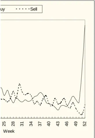
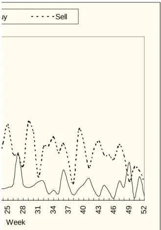
Figure II shows the weekly average of daily buy and sell volume of the issuer as a percentage of its total warrant trading volume. The warrant issuer tends to be more active on the buy side than on the sell side in the early and late life of the warrant but comparably active on the buy and the sell side for the rest of the life of the warrant. Figure III shows that, except toward the end of the life of warrant, in general the warrant issuer is relatively more active on the sell side than on the buy side in the trading of the underlying stock.
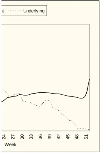
Figure IV depicts the issuer’s weekly inventory position in the warrant and the underlying. The observations in the figure are scaled by the total number of warrants outstanding. For the underlying stock the ratio can be considered as the actual delta of the hedged portfolio. The first observation is the initial inventory before trading on the secondary market starts. The result in the figure is the mean across all warrants. In the beginning the issuer holds about the same number of the underlying stock as that of the warrant, which reflects the fact that the warrant was issued about at the money. As the warrant approaches maturity, the
inventory position of the underlying
diminishes to almost nil. The inventory of warrant increases with time, but as Figure IV shows, the issuer does not buy back all the outstanding warrants. There are a couple of reasons for this phenomenon that relate to risk management and liquidity. One, the ____________________________________
7 The warrant issuers can only submit limit orders for trading. According to Handa and Schwartz (1996) and Berkman (1996), limit order traders issue “free option” to market order traders, thereby providing liquidity to the market.
8 Chow, Hsu and Tso (2001) find that on average 50,000 traders trade on a particular stock during a 18 months period.
issuer can manage its risk exposure by adjusting the stock inventory as the stock price changes and leaving the amount of warrants outstanding intact. Or it can increase the inventory of warrants thereby reducing its risk exposure to the exercise of warrants. Some of the warrants matured deep out of money. So, there is no need for the issuer to buy back the warrant in order to reduce its risk. Two, although buying back warrant can reduce the risk exposure of the issuer, in order to maintain a liquid market the issuer has to keep some warrants outstanding.
We calculate the weekly correlation between the daily inventory change in warrants and the underlying stock. The correlation is the pooled correlation of all the daily observations of all the warrants in our sample. We also calculate the correlation between the weekly inventory change in warrants and the underlying stock. Figure V shows that the correlations are negative in the beginning and toward the end of the life of the warrant but positive in the middle of the life of the warrant. The more negative is the correlation the more likely the issuer adheres to the risk management program that adjusts the stock inventory with the warrant inventory.
To investigate if the issuer makes profits from its trading activities on the warrant market and the underlying market we summarize in Table III their trading profits. We have access to the initial inventory of four warrants. As a result, we can only
calculate the trading profits of the four stocks. Table III shows that the mean and the median of trading profit are negative for the
underlying.
In order to investigate the trading behavior of warrant issuers and its impacts on the price of warrants and stocks we adopt the following sampling approach. We search from the beginning of each trading day for all the warrant trades of the issuer during the trading day. Once we identify a warrant trade, we take observations that occur within the period six minutes before and after the warrant trade of the issuer. We then count the number of different scenarios according to the following rule.
We separate the sample in which the identified warrant trade is a buy and the sample in which the trade is a sell. We then calculate five consecutive percentage price changes in the underlying stocks before and after the issuer trades on the warrants market.9
The observations of price changes are classified into four categories. The first one is the sample in which stock trades of the warrant issuer can be found before the identified trade but no stock trades of the issuer can be found after the identified trade. The second one is the sample in which stock trades of the warrant issuer can be found both before and after the identified trade. The third one is the sample in which stock trades of the warrant issuer cannot be found before the identified trade but stock trades of the issuer can be found after the identified trade. The fourth one is the sample in which no stock trades of the warrant issuer can be found either before or after the identified trade.
For each of the four categories we count the number of warrant trades before and after the identified trade. We further group a category into 16 sub-samples. The first one is the sample that consists of only the issuer’s warrant trades before and after the identified warrant trade. The second one is the sample that consists of only the issuer’s warrant trades before the identified warrant trade but no warrant trades after the identified trade. The third one is the sample that consists of only the issuer’s warrant trades before the identified warrant trade and only the warrant trades of other traders after the identified trade. The fourth one is the sample that consists of only the issuer’s warrant trades before the identified warrant trade and warrant trades of the issuer and other traders
after the identified trade. Other
sub-samples are grouped employing the same logic.
We record the number of observations of each sub-sample. The number of ____________________________________
9
Note that only stocks that are very liquid can be the underlying stocks. As a result, our analysis shows that there are only very few cases in which we cannot find five consecutive price changes within the six minutes window.
observations of each sub-samole would tell us the trading behavior of the issuer. For example, if the issuer usually does not have stock trade before and after the identified warrant trade, then the trading behavior is more like scalper.
The percentage stock price change is calculated as the continuous rate of return of two prices. The first percentage price change after the issuer’s trade is the continuous rate of return between the first stock trade after the issuer’s trade and the trade before the issuer’s trade. The second percentage price change after the issuers trade is the continuous rate of return between the second stock trade and the trade before the issuer’s trade, and so forth. The first percentage price change before the issuer’s trade is the continuous rate of return between the second stock trade before the issuer’s trade and the first trade before the issuer’s trade. The second percentage price change before the issuer’s trade is the continuous rate of return between the third stock trade before the issuer’s trade and the first trade before the issuer’s trade, and so forth.
We also calculate the continuous rate of return of the warrant trades before and after the identified trade. For the period before the identified trade the rate of return is calculated as the natural log of the ratio of the warrant price right before the identified trade and the first warrant price before the identified trade. For the period after the identified trade the rate of return is calculated as the natural log of the ratio of the last warrant price after the identified trade and the warrant price right before the identified trade.
We use a similar sampling procedure to study the stock trade of the issuer. We search from the beginning of each trading day for all the stock trades of the issuer during the trading day. Once we identify a stock trade, we take observations that occur within the period six minutes before and after the stock trade of the issuer. We then count the number of different scenarios according to the following rule. We separate the sample in which the identified stock trade is a buy and the sample in which the trade is a sell. We then calculate five percentage
price changes in the warrants before and after the issuer trades on the stock market.10
The observations of price changes are classified into four categories. The first one is the sample in which warrant trades of the warrant issuer can be found before the identified trade but no warrant trades of the issuer can be found after the identified trade. The second one is the sample in which warrant trades of the warrant issuer can be found both before and after the identified trade. The third one is the sample in which warrant trades of the warrant issuer cannot be found before the identified trade but warrant trades of the issuer can be found after the identified trade. The fourth one is the sample in which no warrant trades of the warrant issuer can be found either before or after the identified trade.
For each of the four categories we count the number of stock trades before and after the identified trade. We further group a category into 16 sub-samples. The first one is the sample that consists of only the issuer’s stock trades before and after the identified stock trade. The second one is the sample that consists of only the issuer’s stock trades before the identified stock trade but no stock trades after the identified trade. The third one is the sample that consists of only the issuer’s stock trades before the identified stock trade and only the stock trades of other traders after the identified trade. The fourth one is the sample that consists of only the issuer’s stock trades before the identified stock trade and stock trades of the issuer and other traders after the identified trade. Other sub-samples are grouped employing the same logic.
We record the number of observations of each sub-sample. The number of observations of each sub-sample would tell us the trading behavior of the issuer. For example, if the issuer usually have warrant trade before and after the identified stock ____________________________________
10 Note that only stocks that are very liquid can be the underlying stocks. As a result, our analysis shows that there are only very few cases in which we cannot find five consecutive price changes within the six minutes window.
trade, then the trading behavior is more like position trader and designated market maker.
The percentage warrant price change is calculated as the continuous rate of return of two prices. The first percentage price change after the issuer’s trade is the continuous rate of return between the first warrant trade after the issuer’s trade and the warrant trade before the issuer’s trade. The second percentage price change after the issuers trade is the continuous rate of return between the second warrant trade and the warrant trade before the issuer’s trade, and so forth. The first percentage price change before the issuer’s trade is the continuous rate of return between the second warrant trade before the issuer’s trade and the first warrant trade before the issuer’s trade. The second percentage price change before the issuer’s trade is the continuous rate of return between the third warrant trade before the issuer’s trade and the first warrant trade before the issuer’s trade, and so forth.
We also calculate the continuous rate of return of the stock trades before and after the identified trade. For the period before the identified trade the rate of return is calculated as the natural log of the ratio of the stock price right before the identified trade and the first stock price before the identified trade. For the period after the identified trade the rate of return is calculated as the natural log of the ratio of the last stock price after the identified trade and the stock price right before the identified trade.
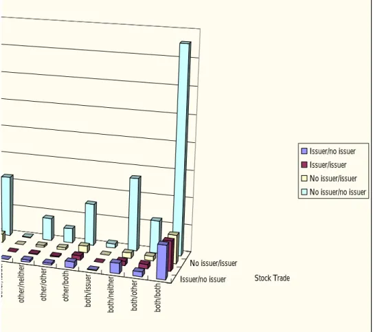
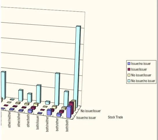
Figures VIA-VID summarizes the number of occurrences of each sample category for warrant and stocks as well as for the identified trade being buy and sell, respectively. Overall we identify more warrant trades than stock trades. In addition, consistent with our observation in Figure II and III, there are more buy transactions than sell ones for warrants but more sell than buy transactions for stocks. Figures VIA and VIB show that about 80% of the time it does not trade the underlying during the period six minutes before and after the issuer buys or sells warrant. And if the issuer trades warrants during the period six minutes before and after it trades warrant, it mainly happens when the issuer does not trade on the
underlying market. In this case about 75% of the time the issuer would trade warrant before or after it has another warrant trade. This finding suggests that the issuer’s decision to trade warrant is not triggered by the events on the underlying market and that if it trades warrant, the trade is not an isolated incident. Combining this finding with what we observe in Figures IV and V, we conclude that the issuer does not follow a strict inventory approach to hedge its warrant risk exposure. In addition, even if the issuer arbitrages between the warrant and the underlying markets it rarely does so.
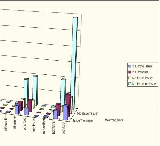
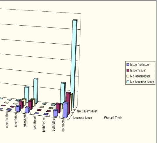
Figures VIC and VID show that about 60% of the time it does not trade warrant during the period six minutes before and after the issuer buys or sells the underlying. And if the issuer trades the underlying during the period six minutes before and after it trades the underlying, it mainly happens when the issuer does not trade on the warrant market. In this case about 85% of the time the issuer would trade stock before or after it has another stock trade. This finding suggests that the issuer’s decision to trade the underlying is relatively independent of the events on the warrant market and that if it trades the underlying, the trade is not an isolated incident. However, comparing Figures VIA and VIB to Figures VIC and VID, one can see that the issuer is less likely to trade stock when it trades warrant than to trade warrant when it trades stocks. This means that if the issuer arbitrages, the arbitrage is more likely to be triggered by the event on the underlying market than that on the warrant market. We think that this finding points more to arbitrage than hedge activity because the issuer usually hedge by adjusting the underlying as the warrant position changes, or by adjusting the underlying inventory as the price of the underlying changes. Finally, Figures I, II, and VIA-VID indicate that the issuer mainly trades on the warrant market like a scalper rather than a position trader or a designated market maker because it participates in transactions quite frequently but rarely trades on both the warrant and the underlying markets simultaneously.
between the price change of the underlying (warrant) and identified warrant (underlying)
trade. According to our sample
classification, if the issuer behaves like a designated market maker on the warrant market, it should trade on the underlying market soon after it trades. This is the “no issuer/issuer” case for the identified trade being a warrant trade. Since the trade is mainly for hedging the warrant risk, the price of the underlying needs not to be significantly affected. If the issuer behaves like a position trader on the warrant market, its warrant trade should be triggered by the price change on the underlying market. This is the “issuer/ no issuer” or the “issuer/issuer” case for the identified trade being a warrant trade. Since a position trader’s volume is usually much greater than that of the designated market maker, the price change before and after the warrant trade should be quite big. If the issuer behaves like a scalper on the warrant market, its warrant trade should not be related to the price change on the underlying market. This is the “no issuer/ no issuer” case for the identified trade being a warrant trade.
On the other hand, if the issuer behaves like a designated market maker on the warrant market, it should trade on the warrant market shortly before it trades on the underlying market. This is the “issuer/no issuer” case for the identified trade being a stock trade. Since the trade is mainly for hedging the warrant risk, the price change of warrant needs not to be big. If the issuer behaves like a position trader on the warrant market, its stock trade should be triggered by the price change on the warrant market. This is the “ no issuer/issuer” or the “issuer/issuer” case for the identified trade being a stock trade. Since a position trader’s volume is usually much greater than that of the designated market maker, the price change before and after the stock trade should be quite big. If the issuer behaves like a scalper on the warrant market, its stock trade should not be related to the price change on the warrant market. This is the “no issuer/ no issuer” case for the identified trade being a stock trade.
Tables IV (V) show the the culumative
rate of return of the six stock trades before and after the identified warrant (stock) trade. When the identified warrant trade is a buy trade in the issuer/no issuer case, there are significant negative returns after the warrant trade. When the identified warrant trade is a buy trade in the issuer/issuer case, there are significant positive returns before the warrant trade. When the identified warrant trade is a buy trade in the no issuer/no issuer case, there are significant negative returns after the warrant trade. When the identified warrant trade is a sell trade in the issuer/issuer case, there are significant negative returns before the warrant trade. When the identified warrant trade is a sell trade in the no issuer/issuer case, there are significant positive returns after the warrant trade. When the identified warrant trade is a sell trade in the no issuer/no issuer case, there are significant negative returns before the warrant trade.
When the identified stock trade is a buy trade in the issuer/no issuer case, there are significant positive returns before the stock trade. When the identified stock trade is a buy trade in the issuer/issuer case, there are significant negative returns after the stock trade. When the identified stock trade is a buy trade in the no issuer/issuer case, there are significant positive returns before the stock trade and significant negative returns after the stock trade. When the identified stock trade is a buy trade in the no issuer/no issuer case, there are significant positive returns before the stock trade and significant negative returns after the stock trade. When the identified stock trade is a sell trade in the issuer/no issuer case, there are significant negative returns before the stock trade. When the identified stock trade is a sell trade in the issuer/issuer case, there are significant positive returns after the stock trade. When the identified stock trade is a sell trade in the no issuer/issuer case, there are significant negative returns before the stock trade and significant positive returns after the stock trade. When the identified stock trade is a sell trade in the no issuer/no issuer case, there are significant positive returns after the stock trade.
V. Conclusion
This paper studies the trading behavior of derivative warrant issuers on the Taiwan Stock Exchange. We conclude that the issuers are the major liquidity providers on the warrant market. They contribute about 20% of the total trading volume to the warrant market. About 40% of the warrant trading volume can transpire because of their participation. They also participate in the trade of 4% of the underlying market. Thus, the issue of warrant also helps increase the liquidity of the underlying.
They trade mainly like scalpers rather than position traders or designated market makers. Although overall their inventory of the underlying stock decreases as the
inventory of warrant increases, they do not quickly adjust their underlying inventory as they trade warrant. In this regard, they are not like designated market makers. In addition, rarely do they trade like position traders.
The premium the warrant issuers collect before the start of secondary market trading is the main source of their profits. In general, they lose money from trading on the secondary market. Since in practice the issuers set a higher premium than the
volatility of the underlying stock warrants (Duan), it seems that the practice takes into account the possibility of losing money from the secondary market trading, which allows the issuer to trade more aggressively on the secondary market and as a result provides liquidity. Thus, this finding provides a new insight on the regulation of a market maker’s (underwriter’s) profit. If we allow liquidity providers to charge a high price for their services, the market liquidity could enhance. The trading of the warrant issuers have some impacts on the price of warrants and the underlying.
Appendix
Our method of calculating trading profits is as follows. Let S0 be the amount of
inventory of the underlying stock (in number of shares) at the open of the first trading day of the warrant. Let PS0 be the price of the
underlying stock at the close of the trading day before the first trading day of the warrant.
Let St be the amount of inventory of the
underlying stock at time t. Let PSt be the
price of the underlying stock at time t. Let SBt be the number of shares bought by the
issuer at time t. Let PSBt be the buy price
of the underlying stock at time t. Let SSt be
the number of shares sold by the issuer at time t. Let PSSt be the sell price of the
underlying stock at time t. There are two ways to calculate the profits from trading the underlying stock. The first is what we called the inventory approach. Suppose the value of the inventory at time t+3 is Vt+3,
then:
Vt+3 = St+3 PSt+3 = (S0 + SBt+1 - SSt+2) PSt+3
(1)
The cost of inventory change between time 0 and t+3 is:
Ct+3 = SBt+1 PSBt+1- SSt+2 PSSt+2
(2)
The total gain/lose taking into account the cost of inventory change is:
TG t+3= Vt+3- Ct+3– V0 =
= (S0 + SBt+1 - SSt+2) PSt+3 – (SBt+1
PSBt+1- SSt+2 PSSt+2) – S0 PS0
= [S0PSt+3– S0 PS0 ] + [(SBt+1 - SSt+2)
PSt+3 – (SBt+1 PSBt+1- SSt+2 PSSt+2)] (3)
The first bracketed part of equation (3) is the “change in the value of inventory.” The second bracketed part is the “trading profit,” assuming that the trading imbalance during the period is reversed at the ending price. In the paper we calculate weekly profits, assuming that in the end of a week the
trading imbalance is reversed at the last close price of the week. Another way to calculate the total gain/loss is what we call the trading approach. The gain/loss of the ending inventory from price change is:
Gt+3 = St+3 (PSt+3– PS0) (4)
The gain/loss from trading is:
TR t+3 = SSt+2 PSSt+2- SBt+1 PSBt+1– (S0
-St+3) PS0 (5)
The total gain/lose taking into account the inventory price change and trading is:
TG t+3 = Gt+3 + TR t+3 = St+3 (PSt+3– PS0) +
SSt+2 PSSt+2- SBt+1 PSBt+1– (S0- St+3) PS0
= St+3 PSt+3 + SSt+2 PSSt+2- SBt+1
PSBt+1– S0 PS0 (6)
Equation (3) and (6) are clearly identical. In fact, equation (4) is written under the assumption that St+3 is smaller than S0. One
can verify that when St+3 is greater than S0,
equation (4) ought to be written as the following:
Gt+3 = S0 (PSt+3– PS0) (7)
Equation (5) would be rewritten as the following:
TR t+3 = SSt+2 PSSt+2- SBt+1 PSBt+1– (S0
-St+3) PSt+3 (8)
But TG t+3 would still be the same as
equation (6)
TG t+3 = Gt+3 + TR t+3 = S0 (PSt+3– PS0) +
SSt+2 PSSt+2- SBt+1 PSBt+1– (S0- St+3) PSt+3
= St+3 PSt+3 + SSt+2 PSSt+2- SBt+1
PSBt+1– S0 PS0 (9)
For ease of programming, we take the inventory approach to calculate the gain/loss from trading the underlying stocks.
The profits from trading the warrant need to be calculated with some adjustment to the method for calculating the profits from trading stocks. Let W0 be the amount of
inventory of the warrant (in number of shares) at the open of the first trading day of the warrant and W be the amount of the total issue of the warrant. Then (W-W0) is the
amount that is subscribed by investors before the secondary market for the warrant starts. PW0 be the issue price of the warrant. Let
Wt be the amount of inventory of the
underlying stock at time t. Let PWt be the
price of the warrant at time t. Let WBt be
the number of warrant bought by the issuer at time t. Let PWBt be the buy price of
warrant at time t. Let WSt be the number of
warrant sold by the issuer at time t. Let PWSt be the sell price of warrant at time t.
There are also two ways to calculate the profits from trading warrant. The first is what we called the inventory approach. Suppose the value of the inventory at time t+3 is WVt+3, then:
WVt+3 = Wt+3 PWt+3 = (W0 + WBt+1
-WSt+2) PWt+3 (10)
The cost of inventory change between time 0 and t+3 is:
WCt+3 = WBt+1 PWBt+1- WSt+2 PWSt+2
(11)
The total gain/lose taking into account the cost of inventory change is:
WTG t+3 = WVt+3- WCt+3– WV0 = = (W0 + WBt+1 - WSt+2) PWt+3 – (WBt+1 PWBt+1- WSt+2 PWSt+2) – W0 PW0 (12) = [W0PWt+3– W0 PW0]+[(WBt+1 - WSt+2) PWt+3 – (WBt+1PWBt+1- WSt+2 PWSt+2)](12)
The first bracketed part of equation (3) is the “change in the value of inventory.” The second bracketed part is the “trading profit,” assuming that the trading imbalance during the period is reversed at the ending price. In the paper we calculate weekly profits, assuming that in the end of a week the trading imbalance is reversed at the last close price of the week. However, the value of the beginning inventory is the opportunity cost of holding the inventory because it would have been the income of the issuer had the warrants been purchased by investors before the start of secondary market trading. The last price used for calculating the last weekly trading profit and the change in the value of inventory for the duration of the warrant depends on if the ending inventory is lower than the beginning inventory. If the ending inventory is not lower than the
beginning inventory, then the last price is 0. Otherwise, the last price is the intrinsic value of warrant if it matures in the money or 0 if it matures out of money. Thus the total profit from issuing the warrant if
WG t+3 = PW0 W - WTG t+3
Just like the case of the underlying stock we can calculate the total gain/loss using what we call the trading approach. Since the logic is identical to that of the stock, we will not repeat the calculation of the trading approach. The combined profits from trading the warrant and the underlying stock is thus the following:
WSTG t+3 = WG t+3 + TG t+3 (13) 四、計畫成果自評 本計畫讓我們有機會能夠瞭解認購權 證發行券商的交易行為,進而增進瞭解如 何管理市場以增加市場的效率性及流動 性。本文的結果亦指出未來值得進一步研 究的議題,同時本計畫可作為以後研究的 開端,藉由未來的研究能對認購權證市場 有更深入的理解,以發展認購權證市場。 五、參考文獻
[1] Alkeback, Per and Niclas Hagelin, 1998,
The impact of warrant introductions on the underlying stocks, with a comparison to stock options, Journal of Futures Markets 18, 307-328.
[2] Berkman, Henk, 1996, Large option
trades, market makers, and limit orders,
Review of Financial Studies 9, 977-1002.
[3] Brenner, Menachem, Rafi Eldor and
Shmuel Hauser, 2001, The price of options liquidity, Journal of Finance 56,
789-805.
[4] Chamberlain, T., C. Cheung and C.
Kwan, 1993, Options introduction, market liquidity and stock behavior: Some Canadian evidence, Journal of Business, Finance and Accounting 20,
687-698.
[5] Chan, Kalok, Y. Peter Chung and Herb
Johnson, 1995, The intraday behavior of bid-ask spreads for NYSE and CBOE options, Journal of Financial and Quantitative Analysis 30, 329-346.
[6] Conrad, J., 1989, The price effect of options introduction, Journal of Finance
44, 487-498.
[7] Chow, Edward H., Yi-Tsong Lee,
Jie-Haun Lee, Yu-Jane Liu and Li-Wen Chen, 2000, The relationship between the price of derivative warrants and their underlying stocks in Taiwan, Review of Securities and Futures Markets 12,
109-146 (in Chinese).
[8] Chow, Edward H., Yuen-Lin Hsu and
Tsao-Hsin Tso, 2001, The liquidity providers on the Taiwan Stock Exchange,
Working Paper, National Cheng-Chi
University.
[9] Damodaran, A and L. Lim, 1991, The
effects of option introduction on the underlying stocks return process,
Journal of Banking and Finance 15,
647-664.
[10] Detemple, J. and P. Jorion, 1990, Option
introduction and stock returns, Journal of Banking and Finance 14, 781-801.
[11] Fedenia, Mark and Theoharry
Grammatikos, 1992, Options trading and the bid-ask spread of the underlying stocks, Journal of Business 65, 335-351.
[12] Figlewski, Stephen, 1998, Derivatives
risks, old and new, Brookings-Wharton
Papers on Financial Services 1, 159-217.
[13] Gemmill, G. 1989, Stock options and
volatility of the underlying shares,
Journal of International Securities Markets 3, 15-22.
[14] Gjerde, Oystein and Frode Saettem,
1995, Option initiation and underlying market behavior: Evidence from Norway,
Journal of Futures Markets 15, 881-899.
[15] Green, T. Clifton and Stephen Figlewski,
1999, Market risk and model risk for a financial institution writing options,
Journal of Finance 54, 1465-1499.
[16] Handa, P. and R. A. Schwartz, 1996,
Limit Order Trading, Journal of Finance
51, 1835-1861.
[17] Jameson, Mel and William Wilhelm, 1992, Market making in the options markets and the costs of discrete hedge rebalancing, Journal of Finance 47,
765-779.
[18] Klemkosky, R. and T. S. Maness, 1980,
The impact of options on the underlying
securities, Journal of Portfolio
Management 9,12-18.
[19] Najarian, Jon, 1992, The options trader, an article in the book The Super Traders: Secrets and Successes of Wall Street’s Best and Brightest, Irwin.
[20] Skinner, D. 1989, Option markets and stock return volatility, Journal of Financial Economics 23, 61-78.
[21] Trennepohl, G. L. and W. Dukes, 1979,
CBOE options and stock volatility,
Review of Business and Economic Research 18, 36-48.
15
Table I
Sample Descriptive Statistics
Issue Price Stock Price at Issue Date Issue Date Listing Date
Maturity No. of Issue (in 1000 shares)
Percentage of the Outstanding Underlying Shares 36.100 133.5 1997/8/20 1997/9/4 1998/9/3 22,000 3.47% 11.340 42.0 1997/8/21 1997/9/4 1998/9/3 22,000 1.42% 16.420 69.0 1997/12/9 1997/12/19 1998/12/18 20,000 2.41% 22.720 77.0 1997/12/16 1998/1/5 1999/1/4 20,000 2.98% 21.600 78.5 1997/12/23 1998/1/8 1999/1/7 20,000 4.58% 16.440 68.5 1998/1/16 1998/2/7 1999/2/6 20,000 0.81% 14.875 59.5 1998/1/21 1998/2/12 1999/2/11 20,000 0.64% 36.420 134.5 1998/2/11 1998/2/26 1999/2/25 20,000 3.44% 29.430 109.0 1998/2/17 1998/3/5 1999/3/4 20,000 0.77% 10.820 45.1 1998/3/4 1998/3/16 1999/3/15 20,000 1.81% 25.810 91.0 1998/3/4 1998/3/19 1999/3/18 20,000 0.48% 14.875 70.5 1998/7/7 1998/7/23 1999/7/22 20,000 3.20%
16
Table II
A comparison of the trading behavior of scalpers, position traders and designated market maker.
Position traders Designated Market Makers
Low High
Low High
High Low
17
Table III
Summary Statistics of Weekly Trading Profits
Warrant Underlying
Std. Min Max Mean Median Std. Min Max
8106.10 -24298.23 15528.57 -11495.57 -11083.25 34139.73 -136311.27 206017.90
3873.74 -10662.10 8823.15 -10509.48 -9711.02 31868.03 -105736.06 225908.84
6094.39 -20652.65 10359.05 -9321.22 -10676.00 22166.93 -59483.13 39233.60
18
Table IV
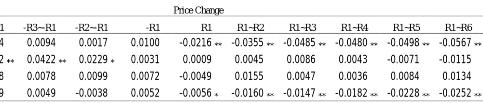
The Mean Cumulative Rate of Returns of the Stock Trades before and after the Identified Warrant Trade Panel A:When the Identified Warrant Trade Is a Buy Trade
Price Change -R4~-R1 -R3~-R1 -R2~-R1 -R1 R1 R1~R2 R1~R3 R1~R4 R1~R5 R1~R6 0.0094 0.0094 0.0017 0.0100 -0.0216 ** -0.0355 ** -0.0485 ** -0.0480 ** -0.0498 ** -0.0567 ** 0.0422 ** 0.0422 ** 0.0229 * 0.0031 0.0009 0.0045 0.0086 0.0043 -0.0071 -0.0115 0.0078 0.0078 0.0099 0.0072 -0.0049 0.0155 0.0047 0.0036 0.0084 0.0134 0.0049 0.0049 -0.0038 0.0052 -0.0056 * -0.0160 ** -0.0147 ** -0.0182 ** -0.0228 ** -0.0252 ** Panel B:When the Identified Warrant Trade Is a Sell Trade
Price Change -R4~-R1 -R3~-R1 -R2~-R1 -R1 R1 R1~R2 R1~R3 R1~R4 R1~R5 R1~R6 -0.0142 -0.0142 -0.0102 0.0028 -0.0130 -0.0185 -0.0103 -0.0082 -0.0144 -0.0186 -0.0413 ** -0.0413 ** -0.0225 -0.0090 -0.0086 0.0242 -0.0026 0.0242 0.0116 0.0047 -0.0146 -0.0146 -0.0064 0.0028 0.0150 0.0364 ** 0.0351 ** 0.0283 * 0.0284 * 0.0192 -0.0215 ** -0.0215 ** -0.0165 ** -0.0035 0.0029 -0.0005 0.0031 0.0022 0.0036 0.0026 Notes: 1. **:5% significant level 2. * :10% significant level
19
Table V
The Mean Cumulative Rate of Returns of the Warrant Trades before and after the Identified Stock Trade Panel A:When the Identified Stock Trade Is a Buy Trade
Price Change -R4~-R1 -R3~-R1 -R2~-R1 -R1 R1 R1~R2 R1~R3 R1~R4 R1~R5 R1~R6 0.0590 * 0.0590 * 0.0226 -0.0385 -0.0118 -0.0352 -0.0186 -0.0428 -0.0439 -0.0439 0.0073 0.0073 0.0103 -0.0496 * -0.1834 ** -0.2858 ** -0.3299 ** -0.3812 ** -0.3794 ** -0.3756 ** 0.0382 ** 0.0382 ** 0.0362 ** 0.0220 * -0.0826 ** -0.2023 ** -0.2568 ** -0.2864 ** -0.2806 ** -0.2811 ** 0.0773 ** 0.0773 ** 0.0710 ** 0.0435 ** -0.0654 ** -0.0728 ** -0.0707 ** -0.0737 ** -0.0811 ** -0.0816 ** Panel B:When the Identified Stock Trade Is a Sell Trade
Price Change -R4~-R1 -R3~-R1 -R2~-R1 -R1 R1 R1~R2 R1~R3 R1~R4 R1~R5 R1~R6 -0.0615 * -0.0615 * -0.0674 -0.0205 -0.0594 -0.0519 -0.0446 -0.0397 -0.0401 -0.0427 0.0543 0.0543 0.0789 ** 0.0557* 0.1887 ** 0.3212 ** 0.3884 ** 0.4353 ** 0.4465 ** 0.4533 ** -0.0962 ** -0.0962 ** -0.0927 ** -0.0736 ** 0.1536 ** 0.1612 ** 0.1828 ** 0.2136 ** 0.2371 ** 0.2479 ** 0.0473 0.0473 0.0459 0.0966 ** 0.0649 ** 0.1223 ** 0.1311 ** 0.1337 ** 0.1466 ** 0.1504 ** Notes: 1. **:5% significant level 2. * :10% significant level
20
Figure I
The Mean Weekly Trading Volume of the Issuers on the Warrant and the Underlying Market Scaled by the Total Trading Volume
0.00 5.00 10.00 15.00 20.00 25.00 30.00 35.00 40.00 1 4 7 10 13 16 19 22 25 28 31 34 37 40 43 46 49 52 Week Warrant Underlying
21
Figure II
The Mean Weekly Buy and Sell Volume of the Issuers on the Warrant Market Scaled by the Total Trading Volume
0.00 5.00 10.00 15.00 20.00 25.00 30.00 35.00 1 4 7 10 13 16 19 22 25 28 31 34 37 40 43 46 49 52 Week Buy Sell
22
Figure III
The Mean Weekly Buy and Sell Volume of the Issuers on the Underlying Market Scaled by the Total Trading Volume
0.00 0.20 0.40 0.60 0.80 1.00 1.20 1.40 1.60 1 4 7 10 13 16 19 22 25 28 31 34 37 40 43 46 49 52 Week Buy Sell
23
Figure IV
The Mean Inventory Position of the Issuers Scaled by the No. of Warrants Issued
0.00 20.00 40.00 60.00 80.00 100.00 120.00 0 3 6 9 12 15 18 21 24 27 30 33 36 39 42 45 48 51 Week Warrant Underlying
24
Figure V
The Correlation between the daily/weekly inventory change in Warrant and the Underlying
-1.0000 -0.8000 -0.6000 -0.4000 -0.2000 0.0000 0.2000 0.4000 0.6000 0.8000 1.0000 1 4 7 10 13 16 19 22 25 28 31 34 37 40 43 46 49 52 Week Daily Weekly
25
Figure VIA
The Mean no. of Observations of Each Sample Category for the Case in which the Identified Trade Is a Warrant Buy
issuer/issuer
issuer/neither issuer/other issuer/both
neither/issuer
neither/neither neither/other neither/both other/issuer
other/neither other/other other/both
both/issuer
both/neither both/other both/both
Issuer/no issuer No issuer/issuer 0.00 50.00 100.00 150.00 200.00 250.00 300.00 350.00 400.00 Stock Trade Issuer/no issuer Issuer/issuer No issuer/issuer No issuer/no issuer
26
Figure VIB
The Mean no. of Observations of Each Sample Category for the Case in which the Identified Trade Is a Warrant Sell
issuer/issuer
issuer/neither issuer/other issuer/both
neither/issuer
neither/neither neither/other neither/both other/issuer
other/neither other/other other/both
both/issuer
both/neither both/other both/both
Issuer/no issuer No issuer/issuer 0.00 50.00 100.00 150.00 200.00 250.00 300.00 Stock Trade Issuer/no issuer Issuer/issuer No issuer/issuer No issuer/no issuer
27
Figure VIC
The Mean no. of Observations of Each Sample Category for the Case in which the Identified Trade Is a Stock Buy
issuer/issuer
issuer/neither issuer/other issuer/both
neither/issuer
neither/neither neither/other neither/both other/issuer
other/neither other/other other/both
both/issuer
both/neither both/other both/both
Issuer/no issuer No issuer/issuer 0.00 20.00 40.00 60.00 80.00 100.00 120.00 Warrant Trade Issuer/no issuer Issuer/issuer No issuer/issuer No issuer/no issuer
28
Figure VID
The Mean no. of Observations of Each Sample Category for the Case in which the Identified Trade Is a Stock Sell
issuer/issuer
issuer/neither issuer/other issuer/both
neither/issuer
neither/neither neither/other neither/both other/issuer
other/neither other/other other/both
both/issuer
both/neither both/other both/both
Issuer/no issuer No issuer/issuer 0.00 50.00 100.00 150.00 200.00 250.00 300.00 Warrant Trade Issuer/no issuer Issuer/issuer No issuer/issuer No issuer/no issuer