適用於具非理想鏈結之無線感測網路之能量效率化分散式最佳線性不偏估計法

國 立 交 通 大 學

電信工程學系碩士班

碩士論文

適用於具非理想鏈結之無線感測網路之

能量效率化分散式最佳線性不偏估計法

Energy-efficient Decentralized BLUE for Wireless

Sensor Networks with Non-ideal Links

研 究 生：陳秋如

Student: Chiu-Ju Chen

指導教授：李大嵩 博士 Advisor:

Dr.

Ta-Sung

Lee

適用於具非理想鏈結之無線感測網路之能量效率化

分散式最佳線性不偏估計法

Energy-efficient Decentralized BLUE for Wireless Sensor

Networks with Non-ideal Links

研 究 生：陳秋如 Student: Chiu-Ju Chen

指導教授：李大嵩 博士 Advisor:

Dr. Ta-Sung Lee

國立交通大學

電信工程學系碩士班

碩士論文

A Thesis

Submitted to Institute of Communication Engineering

College of Electrical Engineering and Computer Science

National Chiao Tung University

in Partial Fulfillment of the Requirements

for the Degree of

Master of Science

in

Communication Engineering

June 2008

Hsinchu, Taiwan, Republic of China

適用於具非理想鏈結之無線感測網路之能量

效率化分散式最佳線性不偏估計法

學生：陳秋如

指導教授：李大嵩 博士

國立交通大學電信工程學系碩士班

摘要

有鑒於低傳送功率對無線感測網路(wireless sensor network)中之感測 器而言為主要需求，如何在有限的總傳送能量下使效能最佳化的設計就愈顯 重要。吾人考慮在一個異質性無線感測網路中利用最佳能量分配策略來對一 個非隨機信號(deterministic signal)做分散式估計。感測器先將其觀測到 之信號取樣成離散訊息後經過瑞利衰減通道(rayleigh fading channel)傳送 至 融 合 中 心 (fusion center) 。 接 著 此 融 合 中 心 利 用 最 佳 不 偏 估 計 (best linear unbiased estimator)融合規則產生最終估計參數。本論文中提出數 種只需得知長期雜訊變異量的統計特性即可求出最佳解之能量分配策略。於 前半部，吾人提出的最佳能量分配策略建議對通道環境不佳或觀測品質不佳 的感測器降低其所傳送訊息之量化解析度或進而將其關掉來節省能量。每個 動態感測器的傳送位元數則由各自的通道衰減、路徑衰減(path loss)、局部 觀測雜訊變異量(local observation noise variance)及能量限制來共同決 定。於後半部，吾人提出兩個疊代式感測器殘餘能量配置演算法，來進一步 提升估計準確度。根據模擬結果，於異質性感測環境中，相較於均衡式能量 分配，吾人所提出的最佳能量分配策略可有顯著的效能改善。

Energy-efficient Decentralized BLUE for Wireless

Sensor Networks with Non-ideal Links

Student:

Chiu-Ju

Chen Advisor:

Dr.

Ta-Sung

Lee

Department of Communication Engineering

National Chiao Tung University

Abstract

As low transmitting power of sensors is a major requirement in wireless sensor networks (WSNs), optimizing their design under energy constraints is of primary importance. We consider an optimal power scheduling problem for the decentralized estimation of a deterministic signal in an inhomogeneous WSN. Sensors quantize their observations into discrete messages, which are transmitted to the fusion center (FC) over rayleigh fading channels. The FC which adopts the best-linear-unbiased-estimator (BLUE) fusion rule generates a final estimate. In this thesis, the optimal power allocation strategies which simply rely on long-term noise variance statistics are presented. In the first part, the proposed power scheduling scheme suggests that the sensors with bad channels or poor observation qualities should decrease their quantization resolutions or simply be shut off to save power. The bit load of each active sensor is determined jointly by individual channel fading gain, path loss, local observation noise variance, and the energy constraint. In the second part, two iterative allocation algorithms of residual energy at sensors are proposed to further enhance estimation accuracy. Numerical results show that in inhomogeneous sensing environments, significant performance improvement is possible when compared to the uniform quantization strategy.

Acknowledgement

I would like to express my deepest gratitude to my advisors, Dr. Ta-Sung Lee and Dr. Jwo Yuh Wu, for their enthusiastic guidance and great patience. I learn a lot from their positive attitude in many areas. Heartfelt thanks are also offered to all members in the Communication System Design and Signal Processing (CSDSP) Lab for their constant encouragement. Finally, I would like to show my sincere thanks to my parents for their invaluable love.

Contents

Chinese Abstract ...I

English Abstract... II

Acknowledgement ... III

Contents ... IV

List of Figures... VI

List of Table ... VIII

Acronym Glossary ... IX

Notations... X

Chapter 1 Introduction... 1

Chapter 2 System Model of Wireless Sensor Network... 4

2.1 Received Signal Model at Sensor Nodes ...5

2.2 Best Linear Unbiased Estimator at Fusion Center...7

2.3 Review of Previous Work ...9

2.4 Summary ...12

Chapter 3 Minimal Mean Square Error Decentralized

Estimation over Rayleigh Fading Channel Based on Sensor

Noise Variance Statistics... 13

3.1 Average Mean Square Error of Decentralized Estimation ...14

3.2 Optimal Closed-form Solution for Sensor Node Resource Allocation...19

3.3 Further Discussions on Optimal Solution ...22

3.4 Computer Simulations ...24

3.5 Summary ...29

Chapter 4 Iterative Allocation of Remaining Energy at Sensor

Nodes ... 31

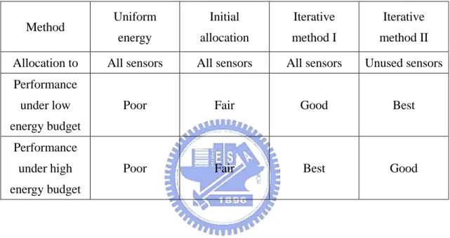
4.1 Method I: Allocation to All Sensor Nodes...32

4.2 Method II: Allocation to Unused Sensor Nodes Only ...38

4.3 Discussions on Proposed Methods ...43

4.4 Computer Simulations ...45

4.5 Summary ...54

Chapter 5 Conclusions and Future Works... 55

Appendices ... 59

List of Figures

Figure 2.1: System Model of Wireless Sensor Network...5

Figure 3.1: Flow chart of initial allocation method ...22

Figure 3.2: Average MSE vs. varying level of total energy...25

Figure 3.3: Average MSE vs. varying noise variance variation factor ...26

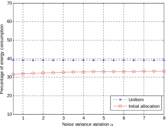
Figure 3.4: Percentage of energy consumption vs. varying noise variance variation factor with low energy budget ...27

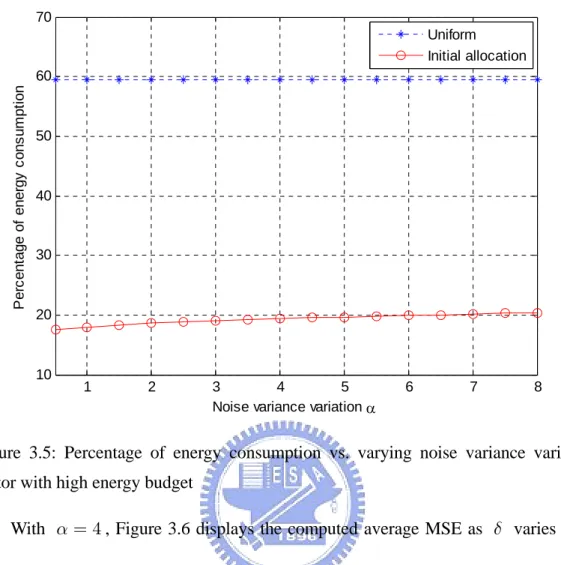
Figure 3.5: Percentage of energy consumption vs. varying noise variance variation factor with high energy budget ...28

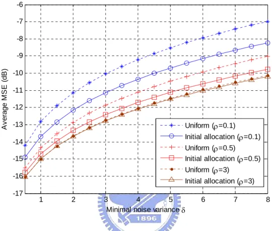
Figure 3.6: Average MSE vs. varying noise variance threshold ...29

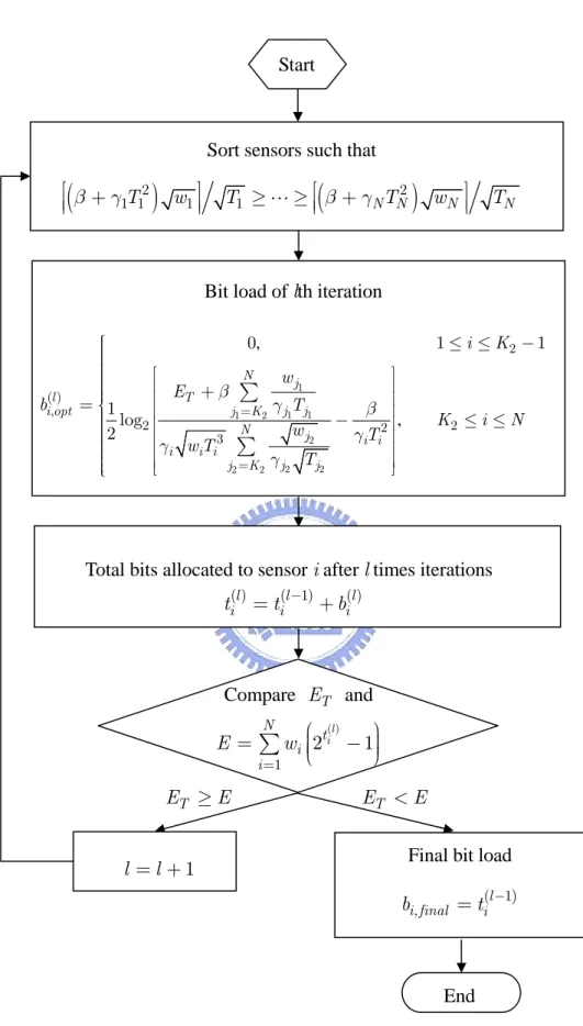
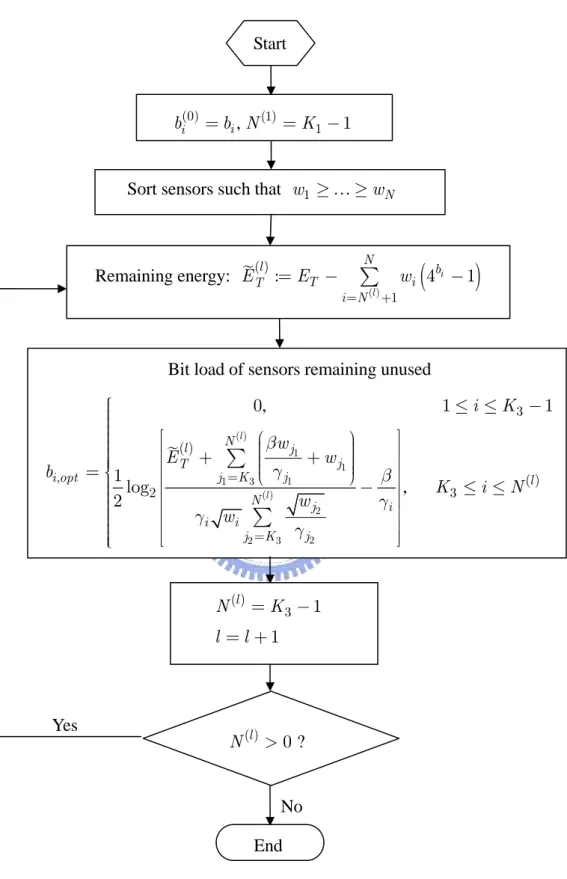
Figure 4.1: Flow chart of method of allocation to all sensor nodes...37

Figure 4.2: Flow chart of method of allocation to unused sensor nodes only ...42

Figure 4.3: Average MSE vs. varying level of total energy...47

Figure 4.4: Average MSE vs. varying noise variance variation factor with low energy budget...49

Figure 4.5: Average MSE vs. varying noise variance variation factor with medium energy budget...49

Figure 4.6: Average MSE vs. varying noise variance variation factor with high energy budget...50 Figure 4.7: Percentage of energy consumption vs. varying noise variance variation

Figure 4.8: Percentage of energy consumption vs. varying noise variance variation factor with medium energy budget ...52 Figure 4.9: Percentage of energy consumption vs. varying noise variance variation

factor with high energy budget ...52 Figure 4.10: Average MSE vs. varying noise variance threshold ...53

List of Table

Acronym Glossary

AWGN additive white Gaussian noise BLUE best linear unbiased estimator BSC binary symmetric channel CSI channel state information DES decentralized estimation scheme

FC fusion center

i.i.d. independent and identically distributed KKT Karush-Kuhn-Tucker MSE mean square error

PDF probability density function QAM quadrature amplitude modulation

SNR signal-to-noise ratio

Notations

α i i δ i T i κ i m N i i q θ i i x

measurement noise variance variation

b number of bits transmitted from the ith sensor

d distance between sensor and the FC i i

d−κ path loss at sensor i

measurement noise variance threshold

E consumed energy for reliable bit decoding at sensor i

E total energy budget

h channel gain between the ith sensor and the FC path loss exponent

output message at the ith sensor number of sensors

n measurement noise at the ith sensor quantization noise at the ith sensor

2

i

n

σ measurement noise variance at the ith sensor

2

i

q

σ quantization noise variance at the ith sensor

2

v

σ channel noise variance deterministic source signal

v additive white channel noise between the ith sensor and the FC local observation at the ith sensor

i

y i

i

z

received signal at the FC from sensor

central Chi-Square distributed random variables with degrees-of-freedom equal to one

Chapter 1

Introduction

The wireless sensor network (WSN) is an emerging technology that has many current and future envisioned applications such as environmental monitoring (air, water, and soil), military surveillance, smart factory instrumentation, space exploration, and so on [1]-[3]. A typical WSN architecture comprises a fusion center (FC) and a large number of geographically distributed sensor nodes. The FC can be either a standard base station or a mobile access point such as an unmanned aerial vehicle hovering over the sensor field. Since sensors are only equipped with small size batteries whose replacement can be rather costly, each sensor node can only transmit a compressed version of its raw measurement to the FC owing to bandwidth and power limitations.

Recently, several decentralized estimation schemes (DESs) [4]-[6] have been proposed for parameter estimation in the presence of additive sensor noise, that is, the local measurement noise. These DESs demand that each sensor node can only transmit a few bits to the FC, with message length determined by each sensor node’s local signal-to-noise ratio (SNR). Performance of the resulting estimator is shown to be within a constant factor of the best linear unbiased estimator (BLUE) performance. The

studies in [7] and [8] present optimal coded and uncoded transmission strategies for WSNs which can minimize the energy consumption per transmitted bit, though the effect of quantization and the accuracy of final estimate are not considered.

Energy efficiency is a critical concern for contemporary sensor network design [9]-[11]. In practical systems, the probability density function (PDF) of the observation noise is hard to characterize, especially for enormous scale sensor networks. In consideration of this limitation, some signal processing algorithms that do not require the knowledge of sensor noise PDF are proposed in [10] and [11]. Seeing that most of the existing related studies require the knowledge of instantaneous noise variance for energy allocation, the proposed approaches instead simply depend on an associated statistical model. In order to enhance the estimation performance against the variation of sensing environments, repeatedly updating the noise profile would be necessary. This comes inevitably at the cost of more training overhead and extra energy consumption. If the sensing environment is harsh, the sensor noise will change expeditiously. Therefore signal processing algorithms proposed in this thesis are required to depend on an associated sensing noise variance model.

In practical WSNs, the wireless channels from sensor nodes to the FC might have different qualities, depending on the sensor nodes’ locations relative to the FC. Intuitively, the local transmitted message length should not only depend on the quality of each sensor node’s observation, that is, local SNR, but also depend on the quality of its wireless channel to the FC. The study in [12] models the channel between each sensor node and the FC as a Rayleigh fading channel. A more inhomogeneous transmitting environment is considered in [13]. The channel impairments, namely path

loss and fading, limit the performance of sensor networks. Although a sensor node has a high quality of observation, it should not perform any local quantization or transmission as long as its channel quality to the FC is not robust enough in order to conserve energy. Moreover, in order to further improve the estimation performance, two advanced energy allocation approaches are also proposed in this thesis. The performance enhancement is conspicuous, though the energy consumption of these strategies is more significant than the proposed initial allocation strategy.

The thesis is organized as follows. In Chapter 2, the system model of WSNs that experiences Rayleigh fading and path loss with BLUE adopted in the FC is introduced. A minimal mean square error (MSE) decentralized estimation scheme based on long-term noise variance knowledge is proposed in Chapter 3. Chapter 4 describes two procedures that iteratively allocate the remaining energy among sensor nodes. The main results are presented and the numerical performance of the proposed approaches are illustrated in this chapter. Finally, the conclusions of this thesis and some potential future works are given in Chapter 5.

Chapter 2

System Model of Wireless Sensor

Network

A common wireless sensor network (WSN) architecture comprises of a fusion center (FC) and a enormous number of geographically distributed sensor nodes which collect observations. Subject to severe energy and bandwidth limitations, each sensor node possesses only limited computation and communication capabilities. It is difficult for sensor nodes to transmit their entire real-valued observations to the FC. In a more practical decentralized estimation scheme (DES), each sensor node preprocesses and extracts information from its raw observations. The information is then aggregated via wireless transmissions at the FC where the received sensor signals are combined to produce a final estimate of the observed quantity. The message lengths are influenced by the power constraint, bandwidth limitation and sensor noise characteristics.

In a practical WSN, the wireless channels from sensor nodes to the FC may have different qualities. The local message length of each sensor node should depend not only on the quality of its local observation, that is, local SNR, but also on the quality of

determined jointly by the local signal-to-noise ratio (SNR) and the quality of its wireless channel to the FC, which is influenced by the fading gain, the path loss, and the noise power. In Section 2.1, the received signal at the FC from each sensor node is discussed. The best linear unbiased estimator (BLUE) is introduced in Section 2.2. Section 2.3 discusses a related previous study. A summary of Chapter 2 is given in Section 2.4.

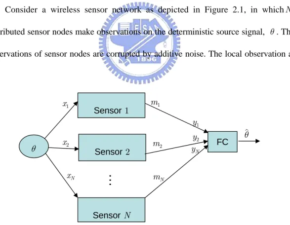
2.1 Received Signal Model at Sensor Nodes

Consider a wireless sensor network as depicted in Figure 2.1, in which distributed sensor nodes make observations on the deterministic source signal, . The observations of sensor nodes are corrupted by additive noise. The local observation at

N θ FC Sensor 1 Sensor 2 Sensor N

…

x₁ x2 x_N y2 mN y_N y₁ m₂ m1 θ θ

the ith node is (2.1) , 1 , i i x = +θ n ≤ ≤i N N

where is independent and identically distributed (i.i.d.) measurement noise with zero-mean and variance . The sensor noise variance is assumed to follow the subsequent relation [9], [10] i n 2 i n σ σ_n2_i (2.2) , , 2 ₁ i n zi i σ = +δ α ≤ ≤

where models the network-wide noise variance threshold, controls the underlying variation from the nominal minimum, and are i.i.d. central Chi-Square distributed random variables each with degrees-of-freedom equal to one, i.e., [14]. 0 δ > α>0

{

z_i :i =1 2, , , … N

}

2 1 i z ∼χ

Owing to the bandwidth limitation and the power constraint, each sensor node ought to quantize its observation into a -bit message. Afterward each sensor node transmits this locally processed data to the FC to generate a final estimate of . In this thesis, the uniform quantization scheme with nearest rounding [15], [16] is adopted. The produced message at the ith sensor node can consequently be modeled as

i b θ (2.3) , 1 , i i i m =x +q ≤ ≤i N

where is the quantization noise which is uniformly distributed with zero mean and variance i q 2 2_{4 i 1} i b q R

σ = − 2 [15], [16]. With the constraint that R >0, _⎢⎡_⎣−R 2,R 2_⎥⎤_⎦ denotes the available signal amplitude range common to all sensor nodes.

Under the flat-fading channel assumption, the received signal at the FC from the

(

)

, , 2 2 2 2 2 1 i i i i i i i i i i i i i i i i i i i y d h m v d h q n v d h d h q d h n v i N κ κ κ κ κ θ θ − − − − − = + = + + + = + + + ≤ ≤ (2.4)

where is the channel gain of the ith communication channel, and is the zero-mean additive channel noise with variance , which is modeled as additive white Gaussian noise (AWGN) . The signal power received at the FC is assumed to be proportional to where is the distance between sensor and the FC, and is the path loss exponent common to all sensor-to-FC links. By collecting all the received data in (2.3) into a vector we have

i h v_i 2 v σ i d−κ d_i i κ

[

]

[

]

[

]

[

, , , , , , , , , , , 1 1 1 : _: : 1 1 : : T T T N N N T N y y h h n n q q v v θ = ₌ = = = ⎡ ⎤ = _{⎣ ⎦} + + + y _h n q v H H … … … … … N

]

T (2.5)

with hi :=d_i−κ2⋅ h_i and H:=diag h

{

⎡_⎣ 1, , … hN⎤_⎦T

}

. Assume that the noise terms in (2.5) are mutually independent and the respective samples ’s, ’s, and ’s are also independent across sensors.

{ , , n q v} i

i

n q_i v

2.2 Best Linear Unbiased Estimator at Fusion

Center

The parameter is retrieved via BLUE [17] in the FC. This estimator simply requires the knowledge of the first and the second moments of the PDF. Assume that the channel state information (CSI) and the local sensor-to-FC path loss can be

observed. Upon receiving sensor messages ’s, the FC combines them into an estimator given by i y θ , 1 1 T T θ = 1 C y−₋ 1 C 1 (2.6)

where is a vector with each element equal to 1 and C is the covariance matrix of the associated noise term:

[1,...,1]Τ =

1

+ +

Hn Hq v . The covariance matrix

of the noise term can therefore be expressed as

( )

( )

( )

. 2 2 2 1 ₁ 2 2 2 2 ₂ 2 2 2 0 0 0 0 0 0 v v N _{N v} h h h σ σ σ σ σ σ ⎡ ₊ ⎤ ⎢ ⎥ ⎢ ⎥ ⎢ ₊ ⎥ ⎢ ⎥ = ⎢ ⎥ ⎢ ⎥ ⎢ ⎥ ⎢ ⎥ + ⎢ ⎥ ⎣ ⎦ C (2.7)

where σ_i2 =σ_n2₁ +σ_q2₁. Thus the final estimate is obtained by

(

)

, 1 2 2 2 2 2 2 2 1 1 1 4 i 4 i i i N N i i b b i i n v i i n v i h y h h h θ σ σ β σ σ β − − − = = ⎛ ⎞ ⎛ ⎞_{⎟⎜ ⎟⎟} ⎜ _⎟⎜ _⎟ ⎜ ⎟⎜ =⎜_{⎜⎜ + +} ⎟_⎟⎟⎜_{⎜ + +} ⎟⎟_⎟ ⎜ ⎟ ⎝

∑

⎠_⎜⎝

∑

⎟_⎠ (2.8)

where β =: R2 12 for notation simplicity. The incurred mean square error (MSE) is thus [16]

( )

(

)

(

)

MSE . 2 1 1 1 2 2 2 1 1 4 i i N b i _{n v} i E h θ θ θ σ σ β − Τ − − − = = − = ⎛ _⎞⎟ ⎜ _⎟ ⎜ _⎟ ⎜ =_⎜⎜ ⎟_⎟ ⎟ + + ⎜ _⎟⎟ ⎜⎝ ⎠

∑

1 C 1 (2.9)

2.3 Review of Previous Work

Adopting the centralized BLUE at the FC was originally proposed in [9]. Thus the FC can perform linear combination of sensor observations to recover . Then the study in [9] proposes an adaptive quantization scheme of sensor observations and discusses its impact on energy saving. The optimal bit loading is obtained via

θ 2 minimize , subject to D'≤D₀. P (2.10) where ₂ 2 1 N i i P = =

_∑

P with denoting the transmit power consumption of sensor , is the achieved MSE performance, and is the target MSE performance. Therefore the following optimization problem based on instantaneous noise characteristics is obtained i P i D' D₀

(

)

(

)

(

)

minimize , subject to , , , , , 2 2 1 1 2 0 _{2 2 2} 0 1 0 2 1 1 ' 1 4 1 i i i i N b i b _i N b i _{n v} i i a D p h b i N σ σ β ∈ ₌ − − = + − ⎛ _⎞⎟ ⎜ _⎟ ⎜ _⎟ ⎜ = + _⎜⎜ ⎟_⎟ ≤ ⎟ + + ⎜ ⎟⎟ ⎜⎝ ⎠ ∈ =

∑

∑

… D i (2.11) where . To facilitate the consequent analyses, the condition is relaxed to . Since the problem is still non-convex, we define

i a =dκ b_i ∈ +₀ i b ∈

(

2

)

, . 2 2 1 1, , 4 i i i _b i n v f h σ σ β − = + + i= … N (2.12)

(

)

(

)

minimize , subject to , < , , , , 2 2 2 2 2 2 1 ' 1 0 2 2 2 4 1 1 1 0 i i N i i i _{i n i v} i N i i i i n v R f a f f h f D f i h σ σ σ σ = = ⎧ ⎫ ⎪ ⎪ ⎪ ⎪ ⎪ ⎪ ⎪ ⎪ ⎨ _{⎡ ⎤}⎬ ⎪ ⎪ ⎪ _⎢ − − _⎥⎪ ⎪ _{⎣ ⎦}⎪ ⎪ ⎪ ⎩ ⎭ ≥ ≤ = +

∑

∑

… 1 N (2.13) where D₀' =D₀

(

1+p₀

)

2.

Since the problem becomes convex, the Lagrangian function can be obtained

(

)

(

)

, , , , , , . 1 1 2 2 ' 2 2 2 1 0 1 1 4 1 _i N N N N i i i i _{i n i v i} i L f f R f a f D f f h λ μ μ λ μ σ σ = = ⎧ ⎫ ⎪ ⎪ ⎪ ⎪ ⎛ ⎞ ⎪ ⎪ _⎟ ⎪ ⎪ ⎜ _⎟ = ⎨_{⎪ ⎡ ⎤}⎬_⎪+ ⎜_⎜ − _⎟⎟− ⎜⎝ ⎠ ⎪ _⎢ − − _⎥⎪ ⎪ _{⎣ ⎦}⎪ ⎪ ⎪ ⎩ ⎭

∑

∑

… … 1 N i i i f =

∑

(2.14)

Equation (2.14) gives the following Karush-Kuhn-Tucker (KKT) conditions

(

)

, 2 2 2 2 2 2 0 4 1 _i i i i i n i v R a f f h λ μ σ σ − − = ⎡ _{− −} ⎤ ⎢ ⎥ ⎣ ⎦ (2.15) , ' 1 0 1 0 N i i f D λ = ⎛ _⎞⎟ ⎜ _{− ⎟=} ⎜ _⎟ ⎜ _⎟ ⎜⎝

∑

⎠ (2.16) , ' 1 0 1 0 N i i f D = − ≥

∑

(2.17) (2.18) 0 λ ≥

(

)

, , ₂ , , , . 2 2 1 0 0 0 1 i i i i i i n v f f i h μ μ σ σ = ≥ ≤ < = + …N (2.19)

Assume that a₁ ≤a₂ ≤…≤a_N, and define

( )

(

)

(

)

, . 1 ' 2 2 2 2 2 2 1 1 0 1 1 1 i i M M i M i _{n v} i i _{n v} i a G M a D h h M N σ σ σ σ − = = ⎛ ⎞ ⎛_{⎟ ⎟} ⎜ _⎟ ⎜ _⎟ ⎜ _⎟ ⎜ _⎟ ⎜ ⎜ = _⎜⎜ ⎟_{⎟ ⎜⎜} − ⎟_⎟ ⎟ ⎟ + + ⎜ ⎟⎟ ⎜ ⎟⎟ ⎜ ⎜ ⎝ ⎠ ⎝ ≤ ≤

∑

∑

⎞ ⎠ (2.20) Let K₁ be the unique sensor number such that f K <

( )

₁ 1 and f K +

(

₁ 1

)

≥1.

Applying simple manipulations of the KKT system leads to

(

)

(

)

, 1 1 2 2 2 2 1 ' 2 2 2 1 0 1 1 2 i i M i i _{n v} i M i _{n v} i a R h D h σ σ λ σ σ = = ⎛ _⎞⎟ ⎜ _⎟ ⎜ _⎟ ⎜ _⎟ ⎜ _{+ ⎟} ⎜ ⎟ ⎜ ⎟ = ⎜_{⎜ ⎟⎟} ⎟ ⎜ _⎟ ⎜ − ⎟ ⎜ _⎟ ⎜ ₊ ⎟ ⎜ ⎟ ⎜⎝ ⎠

∑

∑

(2.21) and

(

)

opt , , , , 2 2 2 1 1 2 i i i i n v a R f h λ σ σ + ⎛ _⎞⎟ ⎜ = _⎜⎜⎝ − _⎟⎟ = ⎠ + i 1… N x (2.22)

where for and ( ) _{for . Equation (2.22) implies that}

the optimal value of is

( )x + =0 x <0 x += x ≥0 i b

(

)

opt opt for for 2 2 2 1 0 2 2 2 log 1 1 4 0 1 log 1 1 2 i i i i i i n v R b f k M R k a h σ ξ σ σ ⎛ _⎞⎟ ⎜ _⎟ ⎜ _⎟ ⎜ _⎟ ⎜ _⎟ ⎜ ⎟ = ⎜_⎜ + _⎡ ⎟_⎟ ⎤ ⎟ ⎜ _⎟ ⎜ ⎢ ₋ ⎥_⎟ ⎜ _{⎢ ⎥⎟} ⎜ _⎟ ⎜⎝ ⎣ ⎦⎠ ≥ + ⎛ _⎞⎟ ⎜ = _{⎜ ⎟⎟} ⎜ + − ⎟ ⎜ _⎟ ⎜ ₊ ⎟ ⎜ _⎟⎟ ⎜⎝ ⎠ 1 M ⎧⎪⎪ ⎪⎪ ⎪⎪ ⎨⎪ _≥ ⎪⎪ ⎪⎪⎪⎩ (2.23) where

(

)

(

)

. 1 1 1 0 _{2 2} 2 ' _{2 2} 2 1 0 1 2 1 1 i i M M i i _{n v} i i _{n v} i a R _h D _h λ ξ σ σ σ σ − = = ⎛ _⎞⎟ ⎜ _⎟ ⎜ _⎟ ⎜ = =_⎜⎜ − ⎟_⎟ ⎟ + + ⎜ _⎟⎟ ⎜⎝ ⎠

∑

∑

Motivated by this, bit allocation according to long term noise characteristics is proposed in the following chapters.

2.4 Summary

The decentralized estimation of a noise-corrupted deterministic parameter is discussed in this chapter. Each sensor node in the WSN collects an observation, computes a local message, and sends it to the FC. Sensor nodes do not communicate with each other. Local quantization at each sensor node is required to reduce the communication cost. An optimal design of the discrete local message functions and the final fusion function depend on the underlying sensor noise distributions. The sensor noises are assumed to be additive, zero-mean, spatially uncorrelated, but otherwise unknown and possibly different among sensor nodes due to varying sensor quality and inhomogeneous sensing environment. The classical BLUE linearly combines the real-valued sensor observations to minimize the MSE. Unfortunately, transmitting real-valued messages is impractical to implement. Finally, a previous study is discussed. In the next chapter, we construct a DES where each sensor node compresses its observation into a small number of bits with length proportional to the local SNR and the channel quality. The resulting compressed bits from different sensor nodes are then collected and combined by the FC to estimate the unknown parameter.

Chapter 3

Minimal Mean Square Error

Decentralized Estimation over

Rayleigh Fading Channel Based on

Sensor Noise Variance Statistics

In this chapter, a problem similar to the problem recently considered [18]: how to find the optimal bit load which minimizes the average distortion under a fixed total energy budget is studied. A key feature common to the existing related studies [4], [9], [10], [19] is that error free transmission is assumed, that is, perfect wireless channels are considered in these studies. The study in [9] formulates the convex optimization problem to derive an optimal bit loading scheme under the mean square error (MSE) constraint with perfect channel. The study in [20] models the noisy channel between each sensor node and the fusion center (FC) as a binary symmetric channel (BSC) with crossover probability controlled by the transmitted bit energy. However, it requires the instantaneous local sensor noise characteristics to formulate the optimization problem.

This chapter contributes a solution to the minimal MSE decentralized estimation with rayleigh fading channel between each sensor node and the FC by exploiting long term noise variance information. The analytic results reveal that under limited energy budget, sensor nodes with unfavorable channel quality or low local SNR should be shut off. The energy distributed to those active sensor nodes should be proportional to the individual channel gain of each active sensor node. In Section 3.1, the average mean square error (MSE) is analyzed. The optimal closed-form solution is provided in Section 3.2. Section 3.3 and Section 3.4 contain discussions and numerical results of the proposed optimal solution. Section 3.5 summarizes this chapter.

3.1 Average Mean Square Error of Decentralized

Estimation

Assume that the ith sensor node transmits its locally processed -bit message, , via applying quadrature amplitude modulation (QAM) with a constellation size . According to [21], the consumed energy for reliable bit decoding is thus

i b i m 2bi

(

2bi 1

)

, 1 , i i E =w − ≤ ≤i N (3.1) where w_i :=σ_v2 hi2 =d_iκ⋅σ_v2 h_i2 and _i w_i i

E is the local signal-to-noise ratio (SNR) received by the FC from the ith sensor node. For a fixed set of the measurement noise

(BLUE), under an permissible total energy budget E_T, can be formulated as

(

)

minimize , subject to , , , 1 2 1 1 0 1 4 2 1 1 i i i N b i n i N b i T i i w w E b i N σ β − − = = + ⎛ _⎞⎟ ⎜ _⎟ ⎜ _⎟ ⎜ _⎟ ⎜ + + ⎟ ⎜⎝ ⎠ − ≤ ∈ ≤ ≤

∑

∑

(3.2) or equivalently,

(

)

maximize , subject to , , , 2 1 1 0 1 4 2 1 1 i i i N b i n i N b i T i i w w E b i N σ β − = = + + + − ≤ ∈ ≤ ≤

∑

∑

(3.3) where +₀ denotes the set of all nonnegative integers.

Toward a solution independent of instantaneous noise conditions, as in [18] and [19], we evaluate the following optimization problem, in which the equivalent distortion cost function in (3.3) is averaged over the noise variance statistic characterized in (2.2): ( )

(

)

maximize , subject to , , , 0 1 : 1 0 1 4 2 1 1 i i N b i i i J N b i T i i p d z w w E b i N δ α β − = = = + + + + − ≤ ∈ ≤ ≤

∑

∫

∑

z z z (3.4) where z=

[

z z₁, , , ₂ … z_N

]

T with p( )z denoting the associated distribution. Since

is a central i.i.d. Chi-Square distributed random variable with

2 1

i

degrees-of-freedom equal to one [14] ( ) , , , . 2 1 2 1 0 2 0 0 z e z z p z z χ π − ⎧⎪⎪ ≥ ⎪⎪ = ⎨ ⎪⎪ < ⎪⎪⎩ (3.5)

The averaged MSE performance can be calculated as

( ) MSE , 1 2 0 1 2 0 1 1 4 1 2 4 1 2 4 i i i i i N b i i i z N i b i i i i z N i b i i i i p d z w e dz z z w e dz z w z δ α β π δ α β π δ α β − = − ∞ − = − ∞ − = = + + + = ⋅ + + + = ⎡ + + + ⎤ ⎢ ⎥ ⎣ ⎦

∑

∫

∑ ∫

∑ ∫

z z z (3.6)

A similar closed-form expression of the cost function in (3.4) can be found in [18] and [19]. The following lemma, with proof presented in Appendix A, provides a closed-form expression of the integral involved in the summation in (3.6).

0

J

Lemma 3.1: The following result holds:

(

)

, 4 2 0 1 4 2 4 bi i _i i w _b N i b i _i e Q w J w δ β α δ β π α δ β − ⎡ _{+ +} ⎤ ₋ ⎢ ⎥ ⎣ ⎦ − = ⎡ ⎤ ⋅ _⎢⎣ + + _⎥ = ⋅ ⎡ _{+ +} ⎤ α ⎦ ⎢ ⎥ ⎣ ⎦

∑

(3.7) where ( ) 2 ₂ : 2 t x e Q x dt π − ∞

=

_∫

is the Gaussian tail function.

From (3.5) and Lemma 3.1, the optimization problem in (3.4) can be equivalently expressed as

(

)

(

)

maximize , subject to , , . 4 2 1 1 0 4 2 4 2 1 1 i bi i i i b w i N b i _i N b i T i i w e Q w w E b i N δ β α δ β α π α δ β − − + + − = = + ⎛ _{⎡ ⎤ ⎟}⎞ ⎜ + + _⎟ ⎜ ⎢_⎣ ⎥_{⎦ ⎟} ⎜ ⋅ _⎜ ⎟_⎟ ⎜ ⎟ ⎜ ⎟⎟ ⎜⎝ ⎠ ⋅ ⎡ _{+ +} ⎤ ⎢ ⎥ ⎣ ⎦ − ≤ ∈ ≤ ≤

∑

∑

(3.8)

Equation (3.8) shows that is unfortunately a highly non-linear (and non-convex) function of the sensor’s bit load . The problem therefore becomes intractable if we stick on direct maximization of . An alternative formulation which is more tractable is proposed and an analytic solution can be obtained. By the following approximation to the Gaussian tail function [22]

0 J i b 0 J ( )

(

)

, 2₂ 1 1 2 1 2 _{1 2} x e Q x x x π _{π π} − − − _π ⎡ ⎤ ⎢ ⎥ ≈ ⎢ ⎥ ⎢ _{− + +} ⎥ ⎢ ⎥ ⎣ ⎦ (3.9)

and some straightforward manipulations, the cost function can thus be approximated by

(

)

(

)

(

)

(

)

(

)

, 4 2 1 2 1 1 1 4 2 4 1 1 4 4 2 bi i _i i i i g _b N i b i _i N b b i i i i e Q g g g g g β α β α π α β π β π β πα β − 4 bi ⎡ ₊ ⎤ ₋ ⎢ ⎥ ⎣ ⎦ − = − − − − = ⎡ ⎤ ⋅ _⎢⎣ + _⎥⎦ ⋅ ⎡ ₊ ⎤ ⎢ ⎥ ⎣ ⎦ ≈ − + + + + +

∑

∑

− i w (3.10)

where . The main advantage of (3.10) is that it leads to an associated lower bound on the reciprocal MSE, , in a more tractable form.

:

i

g = +δ

0

J

Through further modification of variable, the problem can be formulated in the form of convex optimization problem which then yields a closed-form solution. By the inequality equation:

(

4 bi

)

2 2

(

4 bi

) (

4

)

,

i i i

g +β − + πα g +β − ≤ g +β −bi +πα (3.11) the approximated cost function in (3.10) is lower bounded by

(

)

(

)(

)

(

)

(

)

, 0 ₂ 1 _{1 1} 1 1 1 1 1 1 1 2 4 4 1 1 4 4 1 4 4 4 i i i i i i i N i i b i b i N b b i _{i i} N b i _i b N b i i J g g g g g g β β π π πα π β π β πα β α γ β = _{− −} − − − − = − = = = ⎛ ⎞_⎟ ⎛ ⎞_⎟ ⎛ ⎞ ⎜ ⎜ ⎜ − _⎜⎝⎜ + _⎠⎟⎟+ _⎜⎜⎝ + _⎟⎟⎠ + _⎜⎜⎝ + _⎠ ≥ _{⎡ ⎤} − + + _⎢⎣ + + _⎥⎦ = + + = +

∑

∑

∑

∑

4bi β ⎟_⎟⎟ i w (3.12) where . According to (3.12), the optimization problem is thus : i gi γ =α+ =α+ +δ

(

)

maximize , subject to , , . 1 1 0 4 4 2 1 1 i i i b N b i i N b i T i i w E b i N γ β = = + + − ≤ ∈ ≤ ≤

∑

∑

(3.13) To facilitate analysis we first observe that, since , it follows that

. This statement implies that the total energy constraint in (3.13) can be substituted by the following one without violating the overall energy budget requirement:

0 i b ∈ +

(

)

(

1 1 2i 1 4 1 N N b i i i i w w = = − ≤ −

∑

∑

bi

)

T E (3.14)

(

)

, 1 4i 1 N b i i w = − ≤

∑

With the aid of (3.14) and by performing a modification of variable with , the optimization problem finally becomes

: 4bi 1

i

(

)

maximize , subject to , 0, . 1 1 1 1 1 N i i i i N i i T i i B B w B E B i N γ β = = + + + ≤ ≥ ≤ ≤

∑

∑

(3.15) In (3.15), the intermediate variable is relaxed to be a non-negative real number so

as to render the optimization problem tractable. AS long as the optimal real-valued (and hence ) is evaluated, the associated bit loads can therefore be obtained through nearest-integer rounding. The major contribution of the alternative problem formulation (3.15) is that it admits the form of convex optimization and can moreover lead to a closed-form solution, as shown below.

i B i B i b

3.2 Optimal Closed-form Solution for Sensor

Node Resource Allocation

In order to solve the problem in (3.15), let us form the associated Lagrangian as

(

)

(

)

, , , , , , . 1 1 1 1 1 1 N N N N i i i T i i i i i i L B B B w B E B B λ μ μ λ γ β = = ⎛ ⎞ + _{⎜ ⎟⎟} = − ⎜_⎜⎜ − _⎟⎟+ + + ⎝ ⎠

∑

∑

… … 1 N i μ =

∑

(3.16)

The associated set of Karush-Kuhn-Tucker (KKT) conditions [23] are listed as follows:

(

1

)

2 i i 0, 1, , , i i w i B β λ μ γ β − + = = ⎡ _{+ +} ⎤ N ⎣ ⎦ … (3.17) (3.18) 1 0, N i i T i w B E λ = ⎛ _⎞⎟ ⎜ _{− ⎟=} ⎜ _⎟ ⎜ _⎟ ⎜⎝

∑

⎠ (3.19) , 0 λ ≥

(3.20) , , , . 0 0 0 1 i i iB Bi i μ ≥ μ = ≥ ≤ ≤ N Condition (3.17) leads to , 1 i i i i i B w β β γ λ μ γ = − − − (3.21)

According to (3.21), λ and ’s should be determined to fulfill the desired constraints. If , (3.17) implies for all and hence

Since all sensor nodes are turned off under this circumstance, it should be precluded. i μ 0 λ = μ >_i 0 1≤ ≤i N , . 0 1 i B = ≤ ≤i N

The assumption is made without loss of generality.

Corresponding to the previous assumption: , is

demonstrated. Let us define the function

1 2 N w ≥w ≥ ≥w i wi γ =α+ +δ γ₁≥γ₂ ≥ ≥γ_N ( )

(

)

, . 1 1 1 1 2 2 2 : N _j T j j j K N _j K K j j K w E w f K _w K N w β γ γ β γ = = ⎛ _⎞⎟ ⎜ _⎟ ⎜ + _⎜ + _⎟⎟ ⎜ ⎟ ⎝ ⎠ = ≤ ≤ +

∑

∑

1 1 (3.22)

Let 1≤K₁ ≤N be the unique integer such that f K −( ₁ 1)< and f K ≥( ₁) 1. If ( ) 1

f K ≥ for all 1 , we simply set . The existence and uniqueness of such is shown in Lemma 3.2 with proof given in Appendix B

K N

≤ ≤ K =₁ 1

1

K

Lemma 3.2: For the function defined in (3.22), if there exist such that

, then . Furthermore, ( ) f K K₁ 1 ( ) 1 f K ≥ f K +

(

₁ 1

)

≥ 1 f N ≥ always holds. ( ) 1 The optimal and λ_opt B_{i opt,} can be obtained by

(

)

, 1 1 1 1 2 2 N _j j j K opt N 2 2 1 j j T j j K w w E β γ λ β γ γ = = = + +

∑

∑

(3.23)

and , , 1 1 1 1 1 2 1 , 1 0 1 1 . N _j T j i opt j K j N _j i i i j j K i K w E w B K i N w w β γ _β γ γ γ = = ⎧ ≤ ≤ − ⎪⎪ ⎪⎪ _{⎛ ⎞} ⎪ _⎟ ⎪ ⎜_{⎜ ⎟} ⎪ + + ⎟ ⎪ ⎜ _⎟ =⎨_⎪ ⎜_⎝ ⎟_⎠ − − ≤ ≤ ⎪⎪ ⎪⎪ ⎪⎪ ⎪⎩

∑

∑

, 2 2 1 1 1 (3.24)

Since 4bi , the optimal bit load is thus i B = −

(

,

)

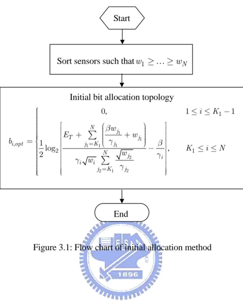
, , . 1 , 2 1 0 1 1 log 1 2 i opt i opt i K b B K i ⎧ ≤ ≤ − ⎪⎪ ⎪ = ⎨_⎪ + ≤ ≤ ⎪⎪⎩ , 1 N i (3.25)

The practical bit load transmitted from the ith sensor node, that is, , can be evaluated via applying nearest-integer rounding to the optimal bit load, . The bit allocation strategy described in this chapter can be illustrated by Figure 3.1. Sensor nodes are initially sorted according tow . Then applying the bit distribution strategy described in Section 3.2 we obtain the bit loading topology.

i

b

,

i opt

Start

Sort sensors such thatw₁≥…≥w_N

Initial bit allocation topology

, , 1 1 1 1 1 2 2 2 1 1 , 2 1 0 1 1 1 log 2 N _j T j j j K i opt N _j i i i j j K i K w E w b K i N w w β γ _β γ γ γ = = ⎧ ≤ ≤ − ⎪⎪ ⎪⎪ _{⎡ ⎛ ⎞ ⎤} ⎪⎪ ⎢ ⎜ ⎟_⎟ ⎥ ⎪ + ⎜ + _⎟ ⎪ ⎢ ⎜ ⎥ ⎪ _⎜ ⎟_⎟ = ⎨_⎪ ⎢ ⎝ ⎠₋ ⎥ _{≤ ≤} ⎢ ⎥ ⎪⎪ ⎢ ⎥ ⎪ _{⎢ ⎥} ⎪⎪ _{⎢ ⎥} ⎪⎪ ⎢_⎣ ⎥_⎦ ⎪⎩

∑

∑

End

Figure 3.1: Flow chart of initial allocation method

3.3 Further Discussions on Optimal Solution

1. Since the path loss is normally much larger than the rayleigh fading gain, sensor which is deployed remote to the FC usually corresponds to the poor background channel gain and therefore large value of . If there are sensor nodes suffer from path losses which vary negligibly, the channel quality is mainly influenced by the rayleigh fading gain. If the sensor nodes are sorted according to , The first sensor nodes are shut off to conserve energy. Similar energy conservation strategies via turning off sensor nodes with poor channel links can be identified in [9], [10], [18], and [19]. From (3.25), the

i i w i w i w K −₁ 1

assigned message length for each active sensor node is inversely proportional to . This is intuitively reasonable while sensor nodes with better channel conditions should be distributed with more bits (and thus more energy) to enhance the estimation accuracy.

i

w

2. The optimization problem described in this chapter merely takes the effect of limited total energy into consideration. In order to prevent sensor nodes from exhausting energy quickly, one intuitive solution is to impose an additional peak energy constraint

(3.26)

(

2bi 1

)

, 1 ,

i P

w − ≤E ≤ ≤ Ni

where E_P is the energy budget per sensor node. By defining a node index set:

(

)

{

,

}

, : 2bi opt 1 1 i P i w E i N

Γ = − > ≤ ≤ , the bit load is thus

(

)

(

)

, , , , and , , and . 1 , 2 1 2 1 0 1 1 log 1 2 log 1 i opt i opt P i i K b B K i N E _{K i N i} w ⎧⎪⎪ _{≤ ≤ −} ⎪⎪ ⎪⎪ ⎪ =_⎨⎪ + ≤ ≤ ∉ Γ ⎪⎪ ⎪⎪ _{+ ≤ ≤ ∈ Γ} ⎪⎪⎩ 1 i (3.27)

This concept can also be applied to the strategies which are described in the next chapter.

3. The practical bit load is evaluated via rounding the optimal real bit load to the nearest integer. Compared to upper-integer rounding and lower-integer rounding, nearest-integer rounding is more closed to the optimal bit load. Thus energy is used more efficiently.

3.4 Computer Simulations

In Section 3.2, an optimal bit allocation scheme is proposed to minimize the reconstruction MSE. The simulated performance of the proposed solution in (3.25) is compared with the scheme of uniform energy allocation with bit load determined via the following equation:

(

2bi 1

)

T , 1 .

i E

w

N

− = ≤ ≤i N (3.28)

In (3.28), is evaluated via applying lower integer rounding so that the resultant total energy can be kept beneath . Therefore it leads to

i b T E , log2 T 1 , i uni i E b Nw ⎢ ⎛_{⎜ ⎞⎟}⎥ ⎢ _⎥⎟ = _⎢ ⎜_⎜ + _⎟⎟⎥ ⎜⎝ ⎠ ⎣ ⎦ (3.29)

where ⎣ ⎦x returns the highest integer that is less than or equal to x . In each

independent simulation we simply choose and which is a uniform distributed random variable with possible values . The total number of trials is 100000 and the number of sensor nodes is set to be 150 in the consequent experiments. The available total energy, that is, energy constraint, is thus

2 κ = d ∈_i [1 10, ] i w , , , 1 2 … 10 (3.30) , 1 N T i E ρ = =

_∑

where ρ is defined as the level of total energy.

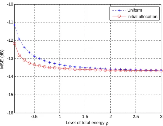
With fixed and , Figure 3.2 displays the computed average MSE as varies from 0.1 to 3. As increases, that is, increases, the estimation performance increases. The proposed solution (3.25) outperforms the uniform energy allocation strategy described in (3.29), especially when is small. Moreover, the

2

δ = α =4

ρ ρ E_T

T

average total energy consumption of the proposed method is less than the uniform energy allocation strategy. The MSE of each scheme saturates as ( ) is larger than a certain value. Under this circumstance, the estimation performance is limited due to the limited number of sensors. This phenomenon will be discussed in Section 4.3. Even though the estimation performance can not be enhanced further, the proposed method still outperforms the uniform energy allocation strategy described in (3.29).

ρ E_T 0.5 1 1.5 2 2.5 3 -16 -15 -14 -13 -12 -11 -10 M S E ( d B)

Level of total energy ρ

Uniform Initial allocation

Figure 3.2: Average MSE vs. varying level of total energy

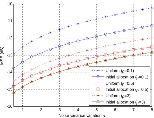
With , Figure 3.3 displays the computed average MSE as varies from 0.5 to 8. Three different levels of total available energy are considered in Figure 3.3. The performance enhancement of the proposed method becomes more significant as

2

the noise variance variation ( α ) gets larger, which means a more inhomogeneous sensing environment. The estimation performance of each strategy degrades while the noise variance variation becomes larger. Moreover, as observed in Figure 3.2, the estimation performance improves as the total available energy increases. The proposed strategy outperforms the uniform energy allocation strategy more significantly under low energy constraint since the proposed strategy allocates energy more efficiently. T E -10 3 1 2 4 5 6 7 8 -16 -15 -14 -13 -12 -11

Noise variance variation α

M S E ( d B) Uniform (ρ=0.1) Initial allocation (ρ=0.1) Uniform (ρ=0.5) Initial allocation (ρ=0.5) Uniform (ρ=3) Initial allocation (ρ=3)

Figure 3.3: Average MSE vs. varying noise variance variation factor

The percentage of energy consumption is defined as

(

)

percentage of energy consumption 1 , 2i 1 N b i i T w E = − =

∑

(3.31)

Where is the bit load allocated to sensor . With , Figure 3.4 and Figure 3.5 display the average percentage of energy consumption for varying from 0.5 to 8. When the energy level is low, the energy consumed by the proposed method is lower than the uniform energy allocation strategy. A similar phenomenon can be observed for high energy level as depicted in Figure 3.5. Although the energy consumption of the proposed method is lower than the uniform energy allocation strategy, the estimation performance of the former is better.

i b i δ =2 α 1 2 3 4 5 6 7 8 10 20 30 40 50 60 70 P e rc en ta ge of e nergy c on s um p ti o n

Noise variance variation α

Uniform Initial allocation

Figure 3.4: Percentage of energy consumption vs. varying noise variance variation factor with low energy budget

1 2 3 4 5 6 7 8 10 20 30 40 50 60 70

Noise variance variation α

P e rc en ta ge of e nergy c on s um p ti o n Uniform Initial allocation

Figure 3.5: Percentage of energy consumption vs. varying noise variance variation factor with high energy budget

With , Figure 3.6 displays the computed average MSE as varies from 0.5 to 8. Three different levels of total available energy are considered in Figure 3.6. The performance enhancement of the proposed method becomes more significant as the minimal noise variance ( ) gets larger, which means that the local SNR degrades. While the minimal noise variance, that is, , increases, the estimation accuracy degrades obviously. The performance degradation is corresponding to lower SNR since the noise variance increases. However, the estimation performance enhancement is more significant as the minimal noise variance increases. As observed in Figure 3.2, the estimation accuracy improves as the total available energy increases. The proposed strategy outperforms the uniform energy allocation strategy more significantly when the energy constraint is extremely small. This phenomenon is

4 α = δ δ δ T E T E

reasonable since the proposed method focus on effectively distributing energy to sensor nodes under stern environments.

1 2 3 4 5 6 7 8 -17 -16 -15 -14 -13 -12 -11 -10 -9 -8 -7 -6

Minimal noise variance δ

A v erag e M S E ( d B ) Uniform (ρ=0.1) Initial allocation (ρ=0.1) Uniform (ρ=0.5) Initial allocation (ρ=0.5) Uniform (ρ=3) Initial allocation (ρ=3)

Figure 3.6: Average MSE vs. varying noise variance threshold

3.5 Summary

In this chapter, a closed-form solution to the minimal-MSE decentralized estimation problem is provided by exploiting a statistical noise variance model. Based on the closed-form expression of the performance measure averaged over the noise variance distribution, MSE minimization becomes a convex optimization problem. The analytic closed-form solution presents the energy saving policy. The proposed solution simply allocates energies to sensor nodes with large channel gains and shut off those

suffering from poor link quality. Numerical simulations reveal that the estimation accuracy is upgraded as total energy increases. The proposed solution outperforms the uniform energy allocation strategy especially when the total available energy is extremely low. Thus the proposed strategy is more effective in an energy-limited environment, which approaches practical wireless sensor network environments.

Chapter 4

Iterative Allocation of Remaining

Energy at Sensor Nodes

In the previous chapter, a tighter energy constraint (3.14) is adopted in order to facilitate the derivation of the closed-form solution (3.25). However, applying the tighter energy constraint might lead to inefficient usage of the available energy resource since the genuine energy consumed by the bit allocation (3.25) could be substantially beneath the energy budget . To remedy this drawback, one approach is to contrive a mechanism for distributing the remaining energy over a certain sensor nodes, thereby the estimation performance can be enhanced further.

T

E

Two procedures for recursively distributing remaining energy are presented in this chapter. The core idea of the first approach proposed is to maximize a certain measure of the incremental increase in the average reciprocal MSE lower bound (3.12) as long as more bits are distributed to sensor nodes. Instead of distributing remaining energy to whole sensor nodes, the second approach proposed mainly focuses on activating sensor nodes which are turned off at present. The first method, namely method of allocation to

all sensor nodes, is introduced in Section 4.1. Then the second method, that is, method of allocation to unused sensor nodes only, is presented in Section 4.2. Section 4.3 makes comparison between these two methods proposed in this thesis. Numerical simulations are exhibited in Section 4.4. Finally, Section 4.5 summarizes this chapter

4.1 Method I: Allocation to All Sensor Nodes

By setting b_i( )0 =b , the ith summand in the summation (3.12), namely, _i

( ) ( ) ( ) , 0 0 0 _: 4 4 i i b i _b i I γ β = + (4.1)

can be regarded as the amount of average MSE reduction contributed by the ith sensor

node with b quantization bits. If extra _i( )0 b bits are allocated to the ith sensor node _i( )1 after the first iteration (hence there are totally b_i( )0 +b_i( )1 bits assigned to this sensor node), I_i( )0 in (4.1) is increased to ( ) ( ) ( ) ( ) ( ) ( ) ( ) ( ) 1 0 0 1 0 0 1 _: 4 4 _. 4 4 i i i i i i i b b b i _{b b b b} i i I γ β γ β + + − = = + + 4 1 (4.2) ( )1 ( )0 i i

I ≥I can be verified since 4bi( )1 ≥ 1. A conceivable criterion for distributing the

remaining energy resource would be directly maximizing the summation, ( )1 .

1 N i i I =

∑

Motivated by this observation, the problem of allocating the remaining energy after l −1 times iterations can be formulated as:

( ) ( ) ( ) ( ) ( ) ( ) ( ) ( ) maximize , subject to , , , , 1 1 1 1 1 1 0 4 4 2 1 1 l l i i l l i i l l i i t b N t b i _i N t b i T i l l i i w E t b i N γ β − − − + + = + = − + + ⎛ _⎞⎟ ⎜ − _⎟≤ ⎜ ⎟ ⎜⎝ ⎠ ∈ ≤ ≤

∑

∑

(4.3) where t_i(l−1) =b_i( )0 + +b_i(l−1) denotes the total bits assigned to the ith sensor node

before the lth iteration begins. The optimization problem in (4.3) is similar to (3.13),

with b_i replaced by t_i(l−1) +b_i( )l . Since b_i( )l ∈ +₀, it follows

(4.4) ( ) ( ) ( ) ( ) ( ) ( ) . 1 1 1 1 1 1 2 1 2 2 4 l l l i i i i l l i i N N t b t b i i i i N _{t b} i i w w w − − − + = = = ⎛ _⎞⎟ ⎜ − _⎟≤ ⎜ ⎟ ⎜⎝ ⎠ ≤

∑

∑

∑

2 l T E

Therefore the total energy constraint in (4.3) can be substituted by the subsequent equation without violating the overall energy budget requirement:

(4.5) ( ) ( ) . 1 1 2il 4il N t b i i w − = ≤

∑

With the aid of (4.5), the optimization problem becomes

maximize , subject to , , , 2 2 1 1 1 1 N _i i i i i i N i i i T i i T B T B w T B E B i N γ β = = + ≤ ≥ ≤ ≤

∑

∑

(4.6) where ( 1) 2til i T = − and ( ) 4bil i

B = for notation simplicity. The iteration index, , is omitted in the formulations below. In order to render the problem tractable, is relaxed to be a non-negative real number.

l

i

In order to solve problem (4.6), we can form the Lagrangian

(

)

(

, , , , , , . 1 1 2 2 1 1 1 1 N N N _i N N i i i i T i i i i i i i i L B B T B w T B E B T B λ μ μ λ γ β = = = ⎛ _⎞⎟ ⎜ _⎟ = − ⎜_⎜⎜ − _⎟⎟+ − + ⎝ ⎠

∑

∑

∑

… …

)

μ (4.7)

The set of KKT conditions [23] then yields:

(

)

, , , , 2 2 2 0 1 i i i i i i i T w T i N T B β _{λ μ} γ +β − + = = … (4.8) (4.9) 1 0, N i i i T i w T B E λ = ⎛ _⎞⎟ ⎜ _{− ⎟=} ⎜ _⎟ ⎜ ⎟ ⎜⎝

∑

⎠ (4.10) , 0 λ≥

(

)

, , , . 0 i 1 0 i 1 1 i i B B i μ ≥ μ − = ≥ ≤ ≤ N (4.11)

Solving for (4.8) leads to

. 2 2 i i i i i i i i i T B T w T T β β γ λ μ γ = − − 2 i N (4.12)

According to (4.12), λ and ’s should be determined to satisfy the desired constraints. If λ , (4.8) implies for all and thus

This circumstance should be precluded since all sensor nodes are turned off. By sorting sensor nodes according to the term:

i μ 0 = μ >_i 0 1≤ ≤i N , . 1 0 1 i B − = ≤ ≤

(

2

)

i iT wi T β γ ⎡ ₊

⎢⎣ ⎤⎥⎦ i and by arranging new indexes to the sensor nodes, the following relationship is obtained:

(

β γ_{1 1}T2

)

w₁ T₁

(

β γ_{N N}T2

)

w_N T_N .

⎡ ₊ ⎤ _{≥ ≥} ⎡ ₊ ⎤

⎢ ⎥ ⎢ ⎥

⎣ ⎦ ⎣ ⎦ (4.13)