高斯-馬可夫衰減通道下雙極傳輸的管道傳輸極限上界

國 立 交 通 大 學

電 信 工 程 學 系 碩 士 班

碩 士 論 文

高斯-馬可夫衰減通道下雙極傳輸的管道

傳輸極限上界

Upper Bounds of Channel Capacity for Bipolar

Transmission Over Gauss-Markov Fading Channel

研 究 生： 蔣名駿

高斯-馬可夫衰減通道下雙極傳輸的管道

傳輸極限上界

Upper Bounds of Channel Capacity for Bipolar

Transmission Over Gauss-Markov Fading Channel

研 究 生： 蔣名駿

Student: Ming-Chun Chiang

指導教授： 陳伯寧 教授

Advisor: Prof. Po-Ning Chen

國 立 交 通 大 學

電 信 工 程 學 系 碩 士 班

碩 士 論 文

A Thesis

Submitted to Institute of Communication Engineering College of Electrical Engineering and Computer Science

National Chiao Tung University in Partial Fulfillment of the Requirements

for the Degree of Master of Science

in

Communication Engineering June 2005

Hsinchu, Taiwan, Republic of China.

高斯-馬可夫衰減通道下雙極傳輸的

管道傳輸極限上界

研究生：蔣名駿 指導教授：陳伯寧 教授

國立交通大學

電信工程學系碩士班

中文摘要

在此篇碩士論文中，我們針對隨時間改變衰減的高斯-馬可夫傳輸管

道，作管道傳輸極限 (capacity) 的探討。首先，我們根據實際通訊系統

的 傳 送 端 與 接 收 端 是 否 分 別具有「頻道狀態資訊」 (channel state

information)，定義出四種不同的管道傳輸極限公式。接著，我們推導高

斯 - 馬 可 夫 傳 輸 管 道 下 的 管 道 輸 出 與 輸 入 信 號 間 的 管 道 轉 換 機 率

(channel transition probability) 公式。由於，在傳送端與接收端均

無「頻道狀態資訊」的情況下，管道傳輸極限的計算相當困難，因此我們

轉而探討其「獨立上界」 (independent bound)。我們導出在不同的管道

記憶級數 (memory order) 下的獨立上界公式，並依公式計算出獨立上界

的數值解加以討論。

Upper Bounds of Channel Capacity for Bipolar

Transmission Over Gauss-Markov Fading Channel

Student: Ming-Chun Chiang Advisor: Prof. Po-Ning Chen

Institute of Communication Engineering

National Chiao-Tung University

Abstract

In this thesis, we focus on the capacity for the time-varying Gauss-Markov fading channels. We first remark on four different definitions of channel capacities according to whether the transmitter and the receiver have or have not the channel state information (CSI). We then provide detailed derivations for the channel transition probability of the Gauss-Markov channels. As the true capacity formula for blind-CSI in both transmitter and receiver is hard to obtain, we derive its independent upper bound instead, and establish a close-form expression of the independent bound for any memory order $M$. Discussions are finally given by numerical evaluation of the independent bounds.

Acknowledgements

I am deeply grateful to my advisor, Prof. Po-Ning Chen, for his encouragement, support and brilliant guidance throughout this research. He always provides many constructive advices and analysis for us in philosophy and research. I greatly appreciate that he is always so patient with us that we can enjoy the research without any pressure. I feel very proud of being his master student.

I would like to thank Prof. Yunghsiang S. Han for his enthusiastic discussion, valuable suggestions and innovative ideas.

I have to thank dear lab-mates, Meng-Yu Wu, Chin-Hui Cheng, Ya-Ting Cho, Chia-Lung Wu, Hsin-Lin Hsieh, Shao-Yu Tseng and Chia-Wei Chang. They often give me precious sug-gestions and are concerned with me, while I am confused and depressed. Most importantly, they help me to understand myself more than ever. I wish that these two memorable years will always make me bear in mind forever.

I would like to give special thanks to my dear friends, Po-Jen Chang, Yu-Shin Chen and Yu-Sheng Lee and Shih-Wei Yeh. They not only talk with me about how to get along with people with patience and sincerity, but also encourage me to live a cheerful life. I really feel lucky to know them.

In the end, I would like to dedicate this thesis to my family, especially my mother and brother (Ming-Tsun), for their love, support and encouragement.

Contents

1.2 Objective of the research . . . 10

1.3 Organization of thesis . . . 11

2 The Definition of Channel Capacity 12 2.1 Capacity definition for memoryless additive channel . . . 12

2.2 Capacity for time-invariant flat fading additive channel . . . 13

2.3 Definition of average capacity C(S) for time-invariant flat fading additive channel . . . 15

2.5 Remarks on four definitions of channel capacities for time-invariant flat fading

additive channel . . . 16

2.6 Capacities for discrete input transmitted over time-invariant flat fading addi-tive channel . . . 18

3 System Model 20 3.1 Data model . . . 20

3.2 Channel model . . . 20

3.3 The statistics of channel state . . . 21

3.4 The channel transition probability of Gauss-Markov fading channel . . . 23

4 Upper Bounds of the Blind-CSI Capacity for Gauss-Markov Fading Chan-nel 24 4.1 Independent bound . . . 24

4.2 Derivation of f (yk|xk) and f (yk) . . . 26

4.3 Independent bound for M = 1 . . . . 33

4.4 Independent bound for M = 2 . . . . 37

4.5 Independent bound for general M . . . . 45

4.6 The lower bound of bit error probability . . . 47

5 Conclusions 51

Appendix 52

List of Tables

List of Figures

4.1 Illustration of Ck(S) for different initial fading coefficients h0 = 0.1, 2 and

10. Other parameters for Gauss-Markov channels are S = 1, C = 1, d = 1,

α = 0.7 and σ2

z = 10. . . 35

4.2 Illustration of Ck(S) for different initial Gauss-Markov fading mean d =

0.5, 1, 3 and 5. Other parameters for Gauss-Markov channels are S = 1,

C = 10, h0 = 1, α = 0.7 and σz2 = 100. . . 36

4.3 Illustration of Ck(S) for different initial fading covariance matrix C = 1, 10

and 100. Other parameters for Gauss-Markov channels are S = 1, h0 = 1,

d = 1, α = 0.7 and σ2

z = 10. . . 37

4.4 f (yk|xk, xk−1) for four different (xk, xk−1). The parameters used in this figure

are s = 1, dk,1= 5.25 + j5.25, dk,2 = 1.75 + j1.75 and Dk,1+ Dk,2+ σz2 = 2. . 44

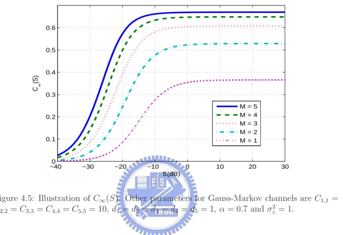
4.5 Illustration of C∞(S). Other parameters for Gauss-Markov channels are

C1,1 = C2,2 = C3,3 = C4,4 = C5,5 = 10, d1 = d2 = d3 = d4 = d5 = 1,

α = 0.7 and σ2

z = 1. . . 46

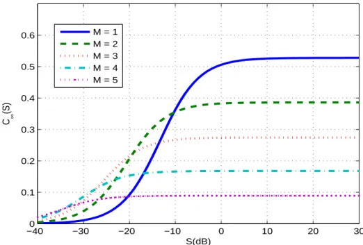
4.6 Illustration of C∞(S). Other parameters for Gauss-Markov channels are

C1,1 = 100.7, C2,2 = 101.5, C3,3 = 102, C4,4 = 102.5, C5,5 = 103, d1 = d2 =

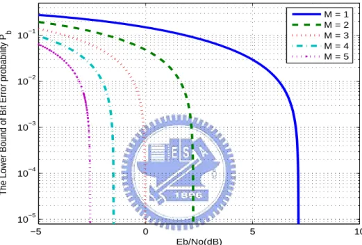
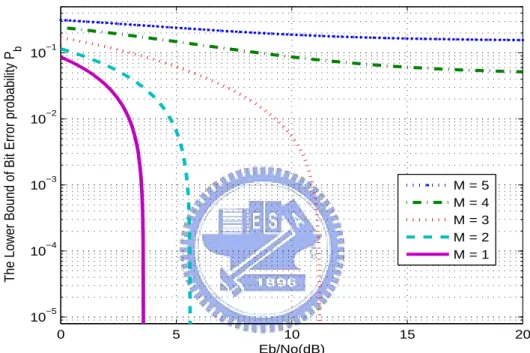
4.7 Illustration of lower bounds for Pb. The code rate adopted is R = 1/3. Other

parameters used in this figure are the same as those in Fig. 4.5. . . 49

4.8 Illustration of lower bounds for Pb. The code rate adopted is R = 1/3. Other

Chapter 1

Introduction

1.1

Problem formulation

Achieving high data-rate transmission at a highly mobile environment is a research challenge in wireless communications. On the one hand, the signal transmitted in air often propagates at a multipath environment so that inter-symbol interferences (ISIs) are introduced to the received signals. On the other hand, fast mobility in time makes these ISIs generally time-varying in nature, which greatly enforce the difficulty of channel estimation at the receiver. Perhaps, the simplest stochastic model for a time-varying channel is the Gauss-Markov [4, 5]. It defines the time-varying ISIs through a discrete-time finite impulse response (FIR) miniature. The question that this thesis aims at is that what the capacity of a time-varying channel, like Gauss-Markov, is. The understanding of this quantity helps the researchers to be fully understood of the gap between the existing technology and the underlying limit.

There have been several publications investigating the capacity of fading channels in the literatures. The capacity of the flat Rayleigh fading channel has been studied in [7, 10] under the assumption that the state of channel fading is perfectly known to both the transmitter and the receiver. While neither the transmitter nor the receiver knows the channel state information (CSI), investigation of the capacity of memoryless Rayleigh fading channels can

be found in [1]. However, seldom publications have been emerged in the capacity study of Gauss-Markov channels.

In [9], the authors addressed in the Introduction Section that perfect and imperfect CSI could have some effect on the capacity quantity. As a consequence, there can be four defi-nitions of channel capacity according to the transmiter/receiver with/without CSI: namely, the capacity when both the transmitter and the receiver knows perfect CSI, the capacity when only the transmitter has perfect CSI, the capacity when only the receiver is perfectly CSI-aware, and the capacity when CSI is unknown to both the transmitter and the receiver. In this thesis, we will remark on these four definitions of capacity, and then turn to the derivations of bounds for the last one.

1.2

Objective of the research

After defining four definitions of channel capacity, we wish to evaluate them based on the Gauss-Markov fading channel model. Unfortunately, the problem of finding the channel input statistics that maximizes the channel input-output mutual information is beyond our management at this stage. Thus, we turn to the determination of good upper bounds for capacities. With the availability of capaicty upper bounds, performance lower bounds to bit error rates (BERs) can be obtained by means of the rate-distortion theorem and the joint source-channel coding theorem [6]. One can then evaluates the performance lower bound numerically in comparison with the simulations of his developed coding scheme. Details will be addressed in subsequent chapters.

1.3

Organization of thesis

This thesis is organized as follows. In Chapter 2, four kinds of definitions of fading channel capacities are introduced, and their operational meanings in practical communication sys-tems are addressed. Chapter 3 introduces the system model. In Chapter 4, upper bounds of the blind-CSI capacity are derived for different channel memory orders, followed by the numerical presentation of their respective performance lower bounds. Chapter 5 concludes this thesis.

Chapter 2

The Definition of Channel Capacity

2.1

Capacity definition for memoryless additive

chan-nel

Let X1, X2, · · · and Y1, Y2, · · · denote the input and output sequences of the channel. In

addition, denote the noise by N1, N2, · · · . Then, a memoryless additive channel could be

defined by:

Yi = Xi+ Ni, i = 1, 2, · · · , (2.1)

where {Xi}∞i=1 and {Ni}∞i=1 are independent random variables, and are also independent

to each other. If {Ni}∞i=1 is assumed to be Gaussian distributed with white power

spec-tral density (PSD), then a memoryless additive white Gaussian noise (AWGN) channel is established.

For discrete input X and discrete output Y , the mutual information can be written as: I (X; Y ) , X x∈X X y∈Y PX,Y (x, y) · log µ PX,Y (x, y) PX(x) · PY (y) ¶ = X x∈X X y∈Y PX(x)PY |X(y|x) · log µ PY |X(y|x) P x0_∈XPX(x0)PY |X(y|x0) ¶ = X x∈X X y∈Y PX(x)PN(y − x) · log    X PN(y − x) x0_∈X PX(x0)PN(y − x0)     . (2.2) Based on this definition, the capacity-cost function for memoryless additive channel with identically distributed {Xi, Ni}∞i=1 subject to input average power constraint E[X2] ≤ S is

given by: C(S) = max {PX : E[X2]≤S} I (X; Y ) = max {PX : E[X2]≤S} X x∈X X y∈Y PX(x)PN(y − x) · log    X PN(y − x) x0_∈X PX(x0)PN(y − x0)     . (2.3)

2.2

Capacity for time-invariant flat fading additive

chan-nel

The channel model for time-invariant flat fading additive channel is defined as:

where H is a time-invariant random variable, independent of {Xi}∞i=1 and {Ni}∞i=1. Then,

the capacity-cost function for time-invariant flat fading channel given [H = h] is equal to:

Ch(S) = max {PX : E[X2]≤S} I (X; Y |h) = max {PX : E[X2]≤S} X x∈X X y∈Y

PX,Y |H(x, y|h) · log

PX,Y |H(x, y|h) PX|H(x|h)PY |H(y|h) = max {PX : E[X2]≤S} X x∈X X y∈Y PX|H(x|h)PY |X,H(y|x, h) · log PX|H(x|h)PY |X,H(y|x, h) PX|H(x|h) X x0_∈X PX,Y |H(x0, y|h) = max {PX : E[X2]≤S} X x∈X X y∈Y PX(x)PN(y − hx) · log PN(y − hx) X x0_∈X PX(x0)PN(y − hx0) , (2.5)

where PX|H is replaced by PX since X is independent of H.

Usually, the average signal-to-noise ratio (SNR) for this channel is given by: SNR = E[E[H

2_X2_|H]]

E[N2_] = E[H

2_]E[X2]

E[N2_].

Therefore, researchers will sometimes fix E[H2_{] = 1, and varies E[N}2_{] to examine the system}

performance of their coding scheme over such a channel.

For continuous channel output alphabet, same derivations can give that:

Ch(S) = max {PX : E[X2]≤S} X x∈X PX(x) Z Y pN(y − Hx) · log pN(y − Hx) X x0_∈X PX(x0)pN(y − Hx0) dy. (2.6) Note that throughout the thesis, we will use the convention that uppercase PX(·) and

low-ercase pX(·) denote the probability mass function (pmf) and probability density function

2.3

Definition of average capacity C(S) for time-invariant

flat fading additive channel

Some researchers focus on the average capacity for fading channel, which is defined as [7]:

C(S) ,

Z

H

pH(h) · Ch(S)dh. (2.7)

The operational meaning of C(S) is that it is the underlying limit for a system in which both the transmitter and the receiver have perfect information about the channel state H. Hence, no matter what H is, the transmitter will always employ the best code that can achieve

Ch(S), and the receiver will use the best decoder corresponding the perfectly estimated

H = h.

It can be easily seen that Eq. (2.7) can be rewritten as:

C(S) = Z H pH(h) · · max {PX : E[X2]≤S} I (X; Y |h) ¸ dh. (2.8) For clarity, let us give an exemplified computation for C(S).

[Example] Suppose that N is Gaussian distributed with zero mean and variance σ2_{. Let}

the channel input alphabet X and output alphabet Y be the real line. Then

Ch(S) = max {PX : E[X2]≤S} I (X; Y |h) = 1 2· log µ 1 + h2· S σ2 ¶ . (2.9)

By assuming that H is Rayleigh distributed with E[H2_{] = σ}2

H, we obtain that: C(S) = Z < h σ2 H · exp µ − h 2 2σ2 H ¶ ·1 2log µ 1 + h 2_{· S} σ2 ¶ dh (2.10) 2

2.4

Definition of capacity C(S) for time-invariant flat

fading additive channel

In the previous section, C(S) is the channel capacity given that the transmitter and the receiver have perfect knowledge of channel state H. In situation where both the transmitter and the receiver are unknown of the channel state, the capacity-cost function should be given by: C(S) , max {PX : E[X2]≤S} I (X; Y ) = max {PX : E[X2]≤S} [h (Y ) − h (Y |X)] = max {PX : E[X2]≤S} X x∈X Z Y pX,Y (x, y) · log µ pX,Y (x, y) PX(x) · pY (y) ¶ dy = max {PX : E[X2]≤S} Z H pH(h) X x∈X Z Y

pX,Y |H(x, y|h) · log

µ pY |X(y|x) pY (y) ¶ dydh = max {PX : E[X2]≤S} Z H pH(h) X x∈X PX(x) Z Y pY |X,H(y|x, h) · log µR H_RpH(h)pY |X,H(y|x, h) HpH(h)pY |H(y|h) ¶ dydh. (2.11)

2.5

Remarks on four definitions of channel capacities

for time-invariant flat fading additive channel

The previous sections have introduced two definitions of channel capacities, namely C(S) and C(S), for time-invariant flat fading additive channel. In fact, we can define four kinds of capacities according to different assumptions on the knowledge that the transmitter and the receiver have. Note that C(S) corresponds to that both the transmitter and the receiver are unaware of the channel state, while C(S) is the capacity under the assumption of perfect

CSI knowledge to both the transmitter and the receiver. Their formulas are listed below. C(S) , max {PX : E[X2]≤S} Z H pH(h) X x∈X PX (x) Z Y pY |X,H(y|x, h) · log µ pY |X(y) pY (y) ¶ dydh (2.12) C(S) , Z H pH(h) max {PX : E[X2]≤S} X x∈X PX (x) Z Y pY |X,H(y|x, h) · log µ pY |X,H(y|x, h) pY |H(y|h) ¶ dydh (2.13)

Now, if only the receiver knows the channel state, the transmitter cannot vary its encoding rule according the channel state. Hence, there can be only one maximization input statistics in the channel capacity formula, and the capacity formula is refined to:

C(R)_{(S) , max} {PX : E[X2]≤S} Z H pH (h) X x∈X PX(x) Z Y pY |X,H(y|x, h) · log µ pY |X,H(y|x, h) pY |H(y|h) ¶ dydh. (2.14)

On the other hand, if only the transmitter is aware of the CSI, the capacity formula will become: C(T )_{(S) ,} Z H pH(h) max {PX : E[X2]≤S} X x∈X PX (x) Z Y pY |X,H(y|x, h) · log µ pY |X(y|x) pY (y) ¶ dydh (2.15) In general, C(S) ≤ C(T )_{(S) ≤ C(S) and C(S) ≤ C}(R)_{(S) ≤ C(S).}

In concept, if a perfect estimate of H is available to the receiver, then the receiver can surely take advantage of the knowledge of pX,Y |H and pY |H at the decoding process. If,

however, the receiver knows nothing about H, it can only use the average counterparts of

pX,Y |H and pY |H in its decoding process, which are exactly:

pY(y) =

Z

H

pH(h) · pY |H(y|h)dh and pX,Y(x, y) =

Z

H

pH(h) · pX,Y |H(y, x|h)dh. (2.16)

This explains why (2.13) and (2.14) use pY |X,H and pY |H in the logarithm term, but (2.12)

Table 2.1: The operational characteristics of four definitions of capacities. Capacity-cost function TX Knows CSI? RX Knows CSI?

C(S) No No

C(T )_{(S) Yes No}

C(R)_{(S) No Yes}

C(S) Yes Yes

In addition, if the transmitter has full knowledge of CSI, the encoding rule can vary according to H; hence, the maximization operation shall be inside the integral with respect

pH. In case the transmitter has no control of CSI, the transmitter can only fix the encoding

rule regardless of the CSI, and hence, the maximization operation shall be placed outside the integral with respect to pH.

These four definitions of capacities are summarized in Tab. 2.1.

2.6

Capacities for discrete input transmitted over

time-invariant flat fading additive channel

In our research, we assume antipodal transmission with input alphabet {−s, +s}, where s can be any real number. Therefore, the power constraint on the input can be simplified to

E[X2_{] = s}2 _{≤ S in the four definitions of capacities, and (2.12)–(2.15) can be re-formulated}

as that: C(S) , max PX∈Pb(S) Z H pH(h) X x∈X PX(x) Z Y pY |X,H(y|x, h) · log µ pY |X(y|x) pY (y) ¶ dydh C(T )_{(S) ,} Z H pH(h) max PX∈Pb(S) X x∈X PX(x) Z Y pY |X,H(y|x, h) · log µ pY |X(y|x) pY (y) ¶ dydh C(R)_{(S) , max} PX∈Pb(S) Z H pH(h) X x∈X PX(x) Z Y pY |X,H(y|x, h) · log µ pY |X,H(y|x, h) pY |H(y|h) ¶ dydh C(S) , Z H pH(h) max PX∈Pb(S) X x∈X PX(x) Z Y pY |X,H(y|x, h) · log µ pY |X,H(y|x, h) pY |H(y|h) ¶ dydh,

Chapter 3

System Model

3.1

Data model

In our system, we assume that binary phase shift keying (BPSK) signaling is transmitted as channel input. The probability of channel input is defined as PX(s) = p and PX(−s) = 1−p,

where p ∈ [0, 1].

3.2

Channel model

A frequency-selective fast fading channel can be modelled by:

yk= xTkhk+ zk = £ xk xk−1 · · · xk−M +1 ¤      hk,1 hk,2 ... hk,M     + zk, k = 1, 2, · · · , n (3.1) where xk = £ xk xk−1 · · · xk−M +1 ¤_T

is the channel input vector consisting of the current input and the previous (M − 1) inputs, M is the time spread or temporal channel memory,

hk =

£

hk,1 hk,2 · · · hk,M

¤_T

is a complex column vector containing the channel impulse response coefficients at time k, and zk is the complex memoryless Gaussian noise at time k

with variance E[zkzk∗] = σz2.

vector at the channel output, transmitted data at the channel input and complex additive noises, respectively. Then, (3.1) can be re-formulated as:

y = Hx + z, (3.2) where H =        h1,M · · · h1,1 0 · · · 0 0 0 0 0 h2,M · · · h2,1 · · · 0 0 0 0 ... ... ... ... ... ... ... ... ... 0 0 0 0 · · · hn−1,M · · · hn−1,1 0 0 0 0 0 · · · 0 hn,M · · · hn,1        . (3.3) Taking M = 3 as an example, we have:

yk = xTkhk+ zk= £ xk xk−1 xk−2 ¤  h_hk,1_k,2 hk,3   + zk, k = 1, · · · , n, (3.4)

which can be reduced to the matrix form as:        y1 y2 y3 ... yn        =        h1,3 h1,2 h1,1 0 · · · 0 0 0 0 0 h2,3 h2,2 h2,1 · · · 0 0 0 0 0 0 h3,3 h3,2 · · · ... ... ... ... ... ... ... ... ... hn−1,3 hn−1,2 hn−1,1 0 0 0 0 0 · · · 0 hn,3 hn,2 hn,1               x−1 x0 x1 ... xn        +        z1 z2 z3 ... zn        . (3.5) According to (3.2), the pdf of the received vector y given x and H is equal to:

f (y|x, H) = 1 (πσ2 z)n n Y k=1 exp à − ¯ ¯yk− xTkhk ¯ ¯2 σ2 z ! . (3.6)

3.3

The statistics of channel state

As aforementioned, if the channel fading is known to the receiver, channel capacity can be evaluated according to either (2.13) or (2.14), depending on whether the transmitter has the information of channel fading or not. In this thesis, we focus more on the channel capacity at the situation that both the transmitter and the receiver are unaware of (and hence do not

need to estimate) the channel state. In such case, we need to compute f (y|x). In principle,

f (y|x) =

Z

H

f (y|x, H) f (H) dH. (3.7) Hence, it remains to define f (H), in addition to (3.6), to establish f (y|x).

A frequently used fading statistics is the Gauss-Markov. It defines the statistics of the fading through a recursive first-order Markovian equation as:

hk= αhk−1+ vk, (3.8)

where vk is complex, white, Gaussian distributed with mean d and covariance matrix C,

and α is a complex-valued scaling constant. The complex-valued constant α is a first-order Markov factor usually chosen according to |α| = e−ωT_{, where T is the system sampling period}

and ω/π is the Doppler spread [4]. Note that the initial channel coefficient h0 is assumed to

be perfectly estimated such that h0 is treated as a known constant. Based on the definition

in (3.8), f (hk|hk−1) is complex Gaussian distributed with mean (αhk−1+ d) and covariance

matrix C. We can therefore express f (H) as:

f (H) = f (h1) n Y k=2 f (hk|hk−1) = 1 |πC|n n Y k=1 exp n − (hk− αhk−1− d)HC−1(hk− αhk−1− d) o . (3.9)

3.4

The channel transition probability of Gauss-Markov

fading channel

Substituting (3.6) and (3.9) into (3.7), we obtain the closed form of probability distribution of f (y|x) in Gauss-Markov fading as:

f (y|x) = 1 (πσ2 z)n|πC|n Z H n Y k=1 " exp à − ¯ ¯yk− xTkhk ¯ ¯2 σ2 z ! exp ³ − (hk− αhk−1− d)HC−1(hk− αhk−1− d) ´i dH = 1 (πσ2 z)n|πC|n " n Y k=1 |πGk| exp à −|yk| 2 σ2 z !# × "_n−1 Y k=1 exph¡q_k− α∗C−1d¢HGk ¡ q_k− α∗C−1d¢− dHC−1d i# × exp h qH nGnqn− (αh0+ d)HC−1(αh0+ d) i , (3.10) where Gk =                  µ x∗ 1xT1 σ2 z + (1 + |α|2_)C−1 ¶−1 , if k = 1 µ x∗ kxTk σ2 z + (1 + |α|2_)C−1_{− |α|}2_C−1_G k−1C−1 ¶−1 , if 1 < k < n µ x∗ nxTn σ2 z + C−1− |α|2_C−1_G n−1C−1 ¶−1 , if k = n (3.11) and q_k =      y1x∗1 σ2 z + C−1_{d + αC}−1_h 0, if k = 1 ykx∗k σ2 z + C−1_{d + αC}−1_G k−1qk−1− |α|2C−1Gk−1C−1d, if 1 < k ≤ n (3.12)

Chapter 4

Upper Bounds of the Blind-CSI

Capacity for Gauss-Markov Fading

Channel

4.1

Independent bound

In this section, we focus on the independent bound of the channel capacity defined similarly in (2.11), i.e. the capacity without knowing the channel fading both at the transmitter and at the receiver. Here, we presume that the channel is reset every n symbols. Therefore,

C(S) , 1

n{Px : 1_ntr(E[xmaxHx])≤S}

I (x; y) , (4.1)

where, as defined in the previous chapter, x = [x2−M, · · · , xn]T, and “tr(·)” denotes the

traverse of a matrix. Since x2−M, · · · , x0 are usually assumed deterministic zero (hence,

they consume no power), and are nothing to do with the information transmission, we will abuse notation x in this chapter as x = [x1, x2, · · · , xn]T without ambiguity. Thus, we can

equivalently replace x by Xn _{to result in:}

C(S) , 1

n{PXn :max1ntr(ΛX)≤S}

where ΛX is the expectation matrix of £ X∗ 1 X2∗ · · · Xn∗ ¤      X1 X2 ... Xn     . By elementary information theory operation [3],

I (Yn_{; X}n_{) =} Z Yn Z Xn pXn_,Yn(xn, yn) log · pXn_,Yn(xn, yn) pYn(yn) p_Xn(xn) ¸ dxn_dyn = Z Yn Z Xn pXn_,Yn(xn, yn) log · pYn_|Xn(yn|xn) pYn(yn) ¸ dxn_dyn = h(Yn_|Xn_{) − h(X}n_{), (4.3)}

where h(·) represents the differential entropy operation. For notational convenience, we will respectively abbreviate pXn_,Yn(xn, yn) and p_Yn(yn) by f (x, y) and f (x) as we did in the

previous chapter.

Although in the previous chapter, the closed form expression for f (y|x) is established, it is still hard to evaluate the capacity in (4.2). An upper bound based on the simple information-theoretical independent bound, however, can be easily obtained. The indepen-dent bound for mutual information is given by:

I (Xn_{; Y}n_{) ≤ I (X} 1; Y1) + · · · + I (Xn; Yn) . (4.4) We then derive: max {PX:1_n P_n i=1E[Xi2]≤S} I (Xn; Yn) ≤ max {PX:1_nPni=1E[Xi2]≤S} [I (X1; Y1) + · · · + I (Xn; Yn)] = max {PX:(∀ i)E[Xi2]≤S} [I (X1; Y1) + · · · + I (Xn; Yn)] (4.5) ≤ max {PX:(∀ i)E[Xi2]≤S} I (X1; Y1) + · · · + max {PX:(∀ i)E[Xi2]≤S} I (Xn; Yn) , (4.6)

where (4.5) holds since in our system setting, every E[X2

i] is equal to s2due to xi ∈ {−s, +s}

for every i. Note that Pn_i=1E[X2

Let Ck(S) denote the maximum of mutual information I(Xk; Yk) under input power

constraints E[X2

k] ≤ S for every k. Then,

C(S) ≤ 1

n[C1(S) + · · · + Cn(S)] . (4.7)

4.2

Derivation of f (y

|x

) and f (y

)

In order to evaluate the independent bound of channel capacity, f (yk|xk) and f (yk) have to

be obtained first. The approach to obtain them can be described as follows. First of all, we derive:

f (yk|x, h1, · · · , hn) , Z C · · · Z C f (y|x, h1, · · · , hn) dy1· · · dyk−1dyk+1· · · dyn = 1 (πσ2 z)n Z C · · · Z C n Y m=1 exp à − ¯ ¯y_m− xT mhm ¯ ¯2 σ2 z ! dy1· · · dyk−1dyk+1· · · dyn = 1 πσ2 z exp à − ¯ ¯y_k− xT khk ¯ ¯2 σ2 z ! = f (yk|xk, hk) , (4.8)

where C denote the set of all complex numbers. Then, we notice that:

f (yk|x) = Z CM · · · Z CM f (yk|x, h1, · · · , hn) f (hn|hn−1) · · · f (h2|h1) f (h1) dh1· · · dhn = Z CM · · · Z CM f (yk|xk, hk) f (hn|hn−1) · · · f (h2|h1) f (h1) dh1· · · dhn = Z CM f (yk|xk, hk) ·Z CM f (hk|hk−1) · · · Z CM f (h2|h1) f (h1) dh1· · · dhk−1 ¸ dhk = Z CM f (yk|xk, hk) f (hk) dhk (4.9)

It remains to find f (hk) for k = 1, · · · , n.

By the system model,

f (h1) = 1 |πC|exp ³ − (h1− αh0− d)HC−1(h1− αh0− d) ´ . (4.10)

Thus, h1 is complex Gaussian distributed with mean d1 , αh0 + d and covariance matrix D1 , C. Next, f (h2) = Z CM f (h2|h1) f (h1) dh1 = 1 |πC| |πD1| Z CM exp ³ − (h2− αh1− d)HC−1(h2− αh1− d) ´ exp ³ − (h1− d1)HD−11 (h1− d1) ´ dh1. (4.11)

The negative exponent inside the integral in (4.11) is:

(h2− αh1− d)HC−1(h2− αh1− d) + (h1− d1)HD−11 (h1− d1) = ((h2− d) − αh1)HC−1((h2− d) − αh1) + (h1− d1)HD−11 (h1− d1) = |α|2hH₁ C−1h1− α (h2− d)HC−1h1− αHhH1 C−1(h2− d) + (h2− d)HC−1(h2− d) +hH₁ D−1₁ h1− dH1 D−11 h1− hH1 D−11 d1+ dH1 D−11 d1 = hH 1 (|α|2C−1+ D−11 )h1+ dH1 D−11 d1+ (h2− d)HC−1(h2− d) − h α (h2− d)HC−1+ dH1 D−11 i h1 − hH1 £ αHC−1(h2− d) + D−11 d1 ¤ = £hH₁ Ω−1₁ h1− µH1 Ω−11 h1− hH1 Ω−11 µ1 ¤ + dH₁ D−1₁ d1+ (h2− d)HC−1(h2− d) = (h1− µ1)HΩ−11 (h1− µ1) − µH1 Ω−11 µ1+ dH1 D−11 d1+ (h2− d)HC−1(h2− d) , (4.12) where µ₁ , Ω1 £ αH_C−1_(h 2− d) + D−11 d1 ¤ and Ω−1 1 , |α|2C−1+ D−11 . In (4.12), only the

first term is relevance to the integrater h1. Hence, taking the first term into (4.11), and

integrating with respect to h1 yields:

Z

CM

exp£−(h1− µ1)HΩ−11 (h1− µ1)

¤

dh1 = |πΩ1| . (4.13)

and µ₁ = 1 β1 £ αH_β 0(h2− d) + d1 ¤

, the remaining terms in (4.12) put:

dH 1 D−11 d1+ (h2− d)HC−1(h2− d) − µH1 Ω−11 µ1 = dH₁ D−1₁ d1+ β0(h2− d)HD−11 (h2− d) − 1 β1 £ αH_β 0(h2− d) + d1 ¤H D−1 1 £ αH_β 0(h2 − d) + d1 ¤ = dH 1 D−11 d1+ β0(h2− d)HD−11 (h2− d) −|α| 2_β2 0 β1 (h2− d)HD−11 (h2− d) − αβ0 β1 (h2− d)HD−11 d1 −αHβ0 β1 dH 1 D−11 (h2− d) − 1 β1 dH 1 D−11 d1 = β0 β1 (h2− d)HD−11 (h2− d) − αβ0 β1 (h2− d)HD−11 d1− αH_β 0 β1 dH₁ D−1₁ (h2− d) +|α| 2_β 0 β1 dH₁ D−1₁ d1 = (h2− d − αd1)HD−12 (h2− d − αd1) ,

where D2 , (β1/β0)D1. Summarizing the above derivation, we obtain:

f (h2) = 1 |πD2| exp h − (h2− αd1− d)HD−12 (h2− αd1− d) i , (4.14) and hence, h2 is complex Gaussian distributed with mean d2 , αd1 + d and covariance

matrix D2.

We now turn to the derivation of f (h3). Observe that

f (h3) = Z CM f (h3|h2) f (h2) dh2 = 1 |πC| |πD2| Z CM exp ³ − (h3− αh2− d)HC−1(h3− αh2− d) ´ exp h − (h2− d2)HD−12 (h2− d2) i dh2, (4.15)

which has the same form as in (4.11). So, the negative exponent inside the integral in (4.15) is likewisely equal to:

= (h2 − µ2)HΩ−12 (h2− µ2) − µH2 Ω−12 µ2+ dH2 D−12 d2+ (h3− d)H C−1(h3− d) , (4.16) where µ₂ , Ω2 £ αH_C−1_(h 3 − d) + D−12 d2 ¤ and Ω−1 2 , |α|2C−1+ D−12 . By observing that C−1 _{= β} 1D−12 and Ω−12 = β2D−12 and µ2 = β12 £ αH_β 1(h3− d) + d2 ¤

, the last three terms in

(4.16), as the first term is removed due to the integration with respect to h2, put:

dH₂ D−1₂ d2+ (h3− d)HC−1(h3− d) − µH2 Ω−12 µ2 = (h3− d − αd2)HD−13 (h3− d − αd2) ,

where D3 = (β2/β1)D2. Hence, h3 is complex Gaussian distributed with mean d3 , αd2+d

and covariance matrix D3.

By repeating the above procedure, we conclude that hk is complex Gaussian distributed

with mean dk = αdk−1 + d and covariance matrix Dk = (βk−1/βk−2)Dk−1 with the initial

values d0 = h0, D0 = C and βk = 1 + |α|2 + · · · + |α|2k with β−1 , 1. As a result,

dk = αkh0+1−α k

1−α d and Dk = βk−1C = 1−|α|2k

1−|α|2 C.

After obtaining the probability distribution of the fading coefficient hk, the probability

distribution of f (yk|x) can be calculated by integrating the product of f (yk|x, hk) and

f (hk) as follows: f (yk|x) = Z CM f (yk|x, hk) f (hk) dhk = 1 πσ2 z 1 |πDk| Z CM exp à − ¯ ¯yk− xTkhk ¯ ¯2 σ2 z ! exp h − (hk− dk)HD−1k (hk− dk) i dhk.(4.17)

The negative exponent in (4.17) is equal to: ¡ yk− xTkhk ¢_H¡ yk− xTkhk ¢ σ2 z + (hk− dk)HD−1_k ¡ hH_k − dk ¢ = |yk| 2 σ2 z − y H kxTk σ2 z hk− hHk x∗ kyk σ2 z + hH_k x ∗ kxTk σ2 z hk+ hHkD−1k hk− hHkD−1k dk −dH k D−1k hk+ dHkD−1k dk = hH_k µ x∗ kxTk σ2 z + D−1_k ¶ hk− hHk µ x∗ kyk σ2 z + D−1_k dk ¶ − µ x∗ kyk σ2 z + D−1_k dk ¶_H hk +dH_kD−1 k dk+ |yk|2 σ2 z = hH kE−1k hk− hHkE−1k ek− eHkE−1k hk+ dHk D−1k dk+ |yk|2 σ2 z = (hk− ek)HE−1_k (hk− ek) − ekHE−1k ek+ dHkD−1k dk+ |yk|2 σ2 z (4.18) where E−1 k , ³ x∗ kxTk σ2 z + D −1 k ´ and ek, Ek ³ x∗ kyk σ2 z + D −1 k dk ´ . Therefore, f (yk|xk) = |πEk| πσ2 z|πDk| exp ( eH kE−1k ek− dHk D−1k dk− |yk|2 σ2 z ) . (4.19)

It remains to simplify the exponent of the above expression. Referring to [11],

¡

A + abH¢−1 = A−1₋ A−1abHA−1

1 + bHA−1a (4.20)

for any k-by-k matrix A, and k × 1 vectors a and b. Hence,

Ek = µ D−1 k + x∗ kxTk σ2 z ¶−1 = Dk− Dkx∗kxTkDk σ2 z + xTkDkx∗k , (4.21) and ek = Ek µ x∗ kyk σ2 z + D−1_k dk ¶ = µ Dk− Dkx∗kxTkDk σ2 z+ xTkDkx∗k ¶ µ x∗ kyk σ2 z + D−1_k dk ¶ (4.22) Also, for any k-by-k0 _{matrix A and k}0_{-by-k matrix B [8],}

where Ik represents the k-by-k identity matrix. This gives that: |πEk| = ¯ ¯ ¯ ¯πDk µ I − x∗kxTkDk σ2 z+ xTkDkx∗k ¶¯_¯ ¯ ¯ = |πDk| ¯ ¯ ¯ ¯I − x∗k xT kDk σ2 z + xTkDkx∗k ¯ ¯ ¯ ¯ = |πDk| ¯ ¯ ¯ ¯1 − x T kDkx∗k σ2 z+ xTkDkx∗k ¯ ¯ ¯ ¯ = |πDk| µ σ2 z σ2 z + xTkDkx∗k ¶ (4.24) By letting σ2

can be reduced to: −eH kE−1k ek+ dHkD−1k dk+ |yk|2 σ2 z = −¡E−1_k ek ¢_H Ek ¡ E−1_k ek ¢ + dH_kD−1_k dk+ |yk|2 σ2 z = − µ x∗ kyk σ2 z + D−1_k dk ¶_Hµ Dk−Dkx ∗ kxTkDk σ2 X ¶ µ x∗ kyk σ2 z + D−1_k dk ¶ + dH_kD−1_k dk+|yk| 2 σ2 z = yH k µ xT kDkx∗kxTkDkx∗k (σ2 z)2σX2 −x T kDkx∗k (σ2 z)2 + 1 σ2 z ¶ yk+ ykH µ dH_kx∗ k µ xT kDkx∗k σ2 zσX2 − 1 σ2 z ¶¶H +dH kx∗k µ xT kDkx∗k σ2 zσX2 − 1 σ2 z ¶ yk+ ¡ xT kdk ¢_H¡ xT kdk ¢ σ2 X = yH k µ (xT kDkx∗k)2 (σ2 z)2σ2X − xTkDkx∗k (σ2 z)2 +σX2 − xTkDkx∗k (σ2 z)2 ¶ yk+ ykH à xT kDkx∗k σ2 z p σ2 X − p σ2 X σ2 z !_H ¡ xT kdk ¢ p σ2 X + ¡ xT kdk ¢_H p σ2 X à xT kDkx∗k σ2 z p σ2 X − p σ2 X σ2 z ! yk+ ¡ xT kdk ¢_H p σ2 X ¡ xT kdk ¢ p σ2 X = "à xT kDkx∗k σ2 z p σ2 X − p σ2 X σ2 z ! yk+ ¡ xT kdk ¢ p σ2 X #_H"à xT kDkx∗k σ2 z p σ2 X − p σ2 X σ2 z ! yk+ ¡ xT kdk ¢ p σ2 X # = ¯ ¯ ¯ ¯ ¯ à xT kDkx∗k σ2 z p σ2 X − p σ2 X σ2 z ! yk+ ¡ xT kdk ¢ p σ2 X ¯ ¯ ¯ ¯ ¯ 2 = 1 σ2 X ¯ ¯ ¯ ¯ µ xT kDkx∗k σ2 z − σ2X σ2 z ¶ yk+ xTkdk ¯ ¯ ¯ ¯ 2 = 1 σ2 X ¯ ¯ ¯ ¯ µ xT kDkx∗k σ2 z − σ2z+ xTkDkx∗k σ2 z ¶ yk+ ¡ xT kdk ¢¯¯ ¯ ¯ 2 = ¯ ¯y_k− xT kdk ¯ ¯2 σ2 z + xTkDkx∗k . (4.25)

Finally, the above derivations summarize to:

f (yk|xk) = |πEk| πσ2 z|πDk| exp à − ¯ ¯y_k−¡xT kdk ¢¯_¯2 σ2 z + xTkDkx∗k ! = |πDk| πσ2 z|πDk| ¯ ¯ ¯ ¯ σ 2 z σ2 z+ xTkDkx∗k ¯ ¯ ¯ ¯ exp à − ¯ ¯y_k−¡xT kdk ¢¯_¯2 σ2 z + xTkDkx∗k ! = 1 π (σ2 z+ xTkDkx∗k) exp à − ¯ ¯yk− ¡ xT kdk ¢¯_¯2 σ2 z + xTkDkx∗k ! , (4.26)

where Dk , (1 − |α|2k)/(1 − |α|2)C and dk , αkh0 + (1 − αk)d/(1 − α). Accordingly, the probability distribution of f (yk) is f (yk) = X xk∈XM PXk(xk) 1 π (σ2 z + xTkDkx∗k) exp à − ¯ ¯yk− ¡ xT kdk ¢¯_¯2 σ2 z + xTkDkx∗k ! . (4.27)

4.3

Independent bound for M = 1

Recall that:

C(S) ≤ 1

n[C1(S) + · · · + Cn(S)] . (4.28)

where Ck(S) = max{PX : (∀ i)E[Xi2]≤S}I(Xk; Yk). Now we will derive Ck(S) for the case of

M = 1. For M = 1, f (yk|xk) = f (yk|xk) = 1 π (σ2 z+ |xk|2Dk) exp à −|yk− xkdk| 2 σ2 z + |xk|2Dk ! = 1 π (σ2 z+ |xk|2Dk) exp à −|dk|2|yk/dk− xk| 2 σ2 z + |xk|2Dk ! . (4.29)

Since I(Xk; Yk) = I(Xk; ˜Yk) for invertible transformation ˜Yk , Yk/dk, we can transform

f (yk|xk) to obtain f (˜yk|xk) as: f (˜yk|xk) = 1 π (σ2 z + |xk|2Dk) /|dk|2 exp à − |˜yk− xk| 2 (σ2 z+ |xk|2Dk)/|dk|2 ! . (4.30)

In our system, the transmitted symbol xkis assumed antipodally modulated. In other words,

xk ∈ {−s, +s} for some real s. In such case, the imaginary part of ˜yk is irrelevant to the

channel input; hence, we can further reduce the complex channel to the real channel without affecting the mutual information as:

f (˜yk,r|xk) = 1 p π(σ2 z+ s2Dk)/|dk|2 exp µ − (˜yk,r − xk) 2 (σ2 z + s2Dk)/|dk|2 ¶ , (4.31)

where ˜yk,r is the real part of ˜yk. For this real-valued symmetric additive Gaussian channel,

its capacity-cost function is achieved by uniform input with s2 _{= S; hence, by denoting}

σ2 N , (σz2+ s2Dk)/(2|dk|2), Ck(S) = I(Xk; ˜Yk,r) = h( ˜Yk,r) − X xk∈X 1 2 Z < f (˜yk,r|xk) log · 1 f (˜yk,r|xk) ¸ d˜yk,r = h( ˜Yk,r) − 1 2log £ 2πeσ2_N¤. (4.32)

Now, for uniform channel input,

h( ˜Yk,r) = − Z < f (˜yk,r) log(f (˜yk,r))d˜yk,r = Z < f (˜yk,r) " 1 2log(2πσ 2 N) + ˜ y2 k,r+ s2 2σ2 N − log à ey˜k,rs/σ2N + e−˜yk,rs/σ2N 2 !# d˜yk,r = 1 2log(2πeσ 2 N) + s2 σ2 N − Z < 1 p 2πσ2 N e−(˜yk,r−s)2/(2σN2)log¡cosh(˜y_k,rs/σ2 N) ¢ d˜yk,r = 1 2log(2πeσ 2 N) + s2 σ2 N − Z < 1 √ 2πe −t2_/2 log à cosh à s2 σ2 N + t s s2 σ2 N !! dt = 1 2log(2πeσ 2 N) + S σ2 N − Z < 1 √ 2πe −t2_/2 log à cosh à S σ2 N + t s S σ2 N !! dt, (4.33)

which immediately gives that:

Ck(S) = 2|dk|2S σ2 z + SDk − Z < 1 √ 2πe −t2_/2 log à cosh à 2|dk|2S σ2 z + SDk + t s 2|dk|2S σ2 z + SDk !! dt. (4.34) By Ces´aro-mean theorem [3], when taking n to infinity, we have:

C(S) ≤ lim n→∞ 1 n n X k=1 Ck(S) = lim n→∞Cn(S) = C∞(S), (4.35) where C∞(S) = 2|d∞|2S σ2 z+ SD∞ − Z < 1 √ 2πe −t2_/2 log à cosh à 2|d∞|2S σ2 z+ SD∞ + t s 2|d∞|2S σ2 z + SD∞ !! dt (4.36)

and d∞= d/(1 − α) and D∞= C/(1 − |α|2), provided that |α| < 1.

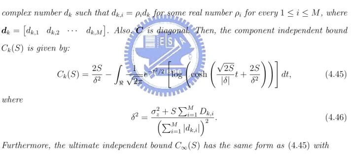
We will demonstrate in the next three figures how channel model parameters affect the independent bound of channel capacity.

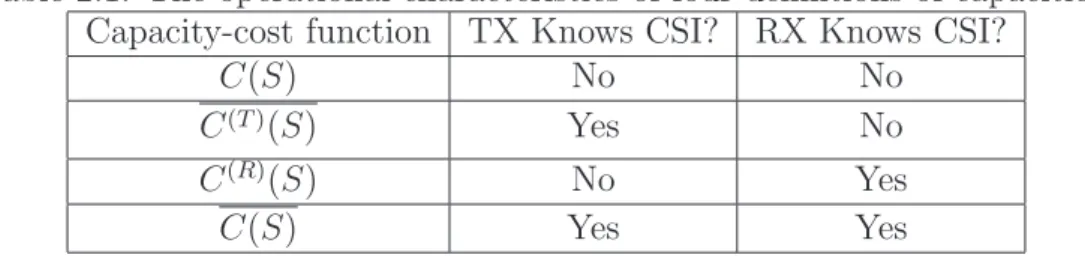
In Fig.4.1, Ck(S) is plotted for different initial channel coefficients h0. Obviously, h0

affects Ck(S) only at small k. As k grows, dk will be dominated by α and d0, and Ck(S)

will converge to the same limit C∞(S).

2 4 6 8 10 12 14 16 18 20 0 0.1 0.2 0.3 0.4 0.5 0.6 k C k (S) C k(S) at C = d = 1, α = 0.7, and σz 2 _{= 10} h 0 = 0.1 h 0 = 2 h 0 = 10

Figure 4.1: Illustration of Ck(S) for different initial fading coefficients h0 = 0.1, 2 and 10.

Other parameters for Gauss-Markov channels are S = 1, C = 1, d = 1, α = 0.7 and σ2

z = 10.

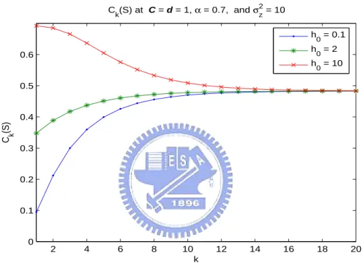
In Fig. 4.2, Ck(S) is plotted for different initial Gauss-Markov fading mean d. In principle,

the value of d determines the strength of line-of-sight (LOS) propagated signal. Figure 4.2 indicates that a stronger LOS signal can result in better capacity bound C∞(S).

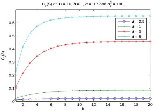
In Fig.4.3, Ck(S) is plotted for different initial fading covariance matrix C. The figure

2 4 6 8 10 12 14 16 18 20 0 0.1 0.2 0.3 0.4 0.5 0.6 k C k (S) C k(S) at C = 10, h = 1, α = 0.7 and σz 2 _{= 100.} d = 0.5 d = 1 d = 3 d = 5

Figure 4.2: Illustration of Ck(S) for different initial Gauss-Markov fading mean d = 0.5, 1, 3

and 5. Other parameters for Gauss-Markov channels are S = 1, C = 10, h0 = 1, α = 0.7

and σ2

z = 100.

An interesting observation that can be made on C∞(S) is that it is equal to zero once

d = 0. This means that the channel capacity C(S) = 0 if there exists no LOS signals in the

communications via Gauss-Markov channels.

The Gauss-Markov channel model can be reduced to the additive white Gaussian noise (AWGN) channel model by letting α = 0, d = 1 and C = 0. As a result,

CAWGN ∞ (S) = CkAWGN(S) = S σ2 z/2 − Z < 1 √ 2πe −t2_/2 log à cosh à S σ2 z/2 + t s S σ2 z/2 !! dt. (4.37)

Notably, this is no longer an upper bound, but the exact channel capacity formula for binary-input AWGN channels [3].

2 4 6 8 10 12 14 16 18 20 0 0.1 0.2 0.3 0.4 0.5 0.6 k C k (S) C k(S) at h = d = 1, α = 0.7 and σz 2 _{= 10.} C = 1 C = 10 C = 100

Figure 4.3: Illustration of Ck(S) for different initial fading covariance matrix C = 1, 10 and

100. Other parameters for Gauss-Markov channels are S = 1, h0 = 1, d = 1, α = 0.7 and

σ2

z = 10.

4.4

Independent bound for M = 2

At M = 2, Ck(S) = max {PX : (∀ i)E[Xi2]≤S} I(Xk; Yk) = max {P_Xk k−1 : E[Xk] 2_{≤S and E[X}2 k−1]≤S} I(Xk; Yk). (4.38)

It is in general hard to find Ck(S) for the case of M > 1. Hence, we made the assumption

on the channel statistics below.

Assumption 4.1 dk,1 = ρ1dk and dk,2 = ρ2dk for some real numbers ρ1 and ρ2, where

dk =

£

dk,1 dk,2

¤

. Also, C is diagonal; hence, there exists Dk,1 and Dk,2 such that

Dk= · Dk,1 0 0 Dk,2 ¸ = (1 − |α|2k)/(1 − |α|2) · C11 0 0 C22 ¸ .

Recall that f (yk|xk) , 1 π (σ2 z + xTkDkx∗k) exp à − ¯ ¯yk− ¡ xT kdk ¢¯_¯2 σ2 z + xTkDkx∗k ! = f (yk|xk, xk−1) = 1 π (σ2 z + |xk|2Dk,1+ |xk−1|2Dk,2) exp à − |yk− xkdk,1− xk−1dk,2| 2 σ2 z+ |xk|2Dk,1+ |xk−1|2Dk,2 ! = 1 π (σ2 z + s2Dk,1+ s2Dk,2) exp à − |yk/dk− (ρ1xk+ ρ2xk−1)| 2 (σ2 z + s2Dk,1+ s2Dk,2)/|dk|2 ! . (4.39)

Then, by letting ˜yk= yk/dk, we obtain:

f (˜yk|xk, xk−1) = 1 πσ2 exp à −|˜yk− (ρ1xk+ ρ2xk−1)| 2 σ2 ! , (4.40) where σ2 _{, (σ}2

z+ s2Dk,1+ s2Dk,2)/|dk|2. By following the same reasoning as in the previous

section,

I(Xk; Yk) = I(Xk; ˜Yk) = I(Xk; ˜Yk,r),

where ˜Yk = ˜Yk,r+ j ˜Yk,i. Then, we derive:

I(Xk; ˜Yk,r) = X xk−1∈X X xk∈X Z < PXk,Xk−1(xk, xk−1)f (˜yk,r|xk, xk−1) log X ¯ xk−1∈X PXk,Xk−1(xk, ¯xk−1)f (˜yk,r|xk, ¯xk−1)   X ˆ xk−1∈X PXk,Xk−1(xk, ˆxk−1)     X x0 k−1∈X X x0 k∈X PXk,Xk−1(x 0 k, x0k−1)f (˜yk,r|x0k, x0k−1)   d˜yk,r;

hence, by taking the derivative of I(Xk; ˜Yk,r) + λ

³P

xk−1∈X

P

xk∈XPXk,Xk−1(xk, xk−1) − 1

with respect to PXk,Xk−1(x 00 k, x00k−1), we obtain: ∂ h I(Xk; ˜Yk,r) + λ ³P xk−1∈X P xk∈XPXk,Xk−1(xk, xk−1) − 1 ´i ∂PXk,Xk−1(x00k, x00k−1) = Z < f (˜yk,r|x00k, x00k−1) log   X ¯ xk−1∈X PXk,Xk−1(x 00 k, ¯xk−1)f (˜yk,r|x00k, ¯xk−1)   d˜yk,r+ 1 − Z < f (˜yk,r|x00k, x00k−1) log   X ˆ xk−1∈X PXk,Xk−1(x 00 k, ˆxk−1)   d˜yk,r− 1 − Z < f (˜yk,r|x00k, x00k−1) log   X x0 k−1∈X X x0 k∈X PXk,Xk−1(x 0 k, x0k−1)f (˜yk,r|x0k, x0k−1)   − 1 + λ = I(x00_k, x00_k−1; ˜Yk,r) − 1 + λ, where I(x00_k, x00_k−1; ˜Yk,r) , Z < f (˜yk,r|x00k, x00k−1) × log X ¯ xk−1∈X PXk,Xk−1(x 00 k, ¯xk−1)f (˜yk,r|x00k, ¯xk−1)   X ˆ xk−1∈X PXk,Xk−1(x 00 k, ˆxk−1)     X x0 k−1∈X X x0 k∈X PXk,Xk−1(x 0 k, x0k−1)f (˜yk,r|x0k, x0k−1)   d˜yk,r By similar reasoning in [3], I(xk, xk−1; ˜Yk,r) ½ = Ck(S), if PXk,Xk−1(xk, xk−1) > 0 ≤ Ck(S), if PXk,Xk−1(xk, xk−1) = 0. (4.41) For notational convenience, let Ik(a, b) denote I(xk = as, xk−1 = bs; ˜Yk,r), where a, b =

±1. Also, brief PXk,Xk−1(xk, xk−1) and f (˜yk,r|xk, xk−1) by pa,b and f (˜yk,r|a, b), respectively.

Then, Ik(a, b) , Z < f (˜yk,r|a, b) log X ¯b=±1 p_a,¯bf (˜yk,r|a, ¯b)  X ˆb=±1 p_a,ˆb   Ã X a0_=±1 X b0_=±1 pa0_,b0f (˜y_k,r|a0, b0) !d˜yk,r

where hk(a, b) , − Z < f (˜yk,r|a, b) log à X a0_=±1 X b0_=±1 pa0_,b0f (˜y_k,r|a0, b0) ! d˜yk,r = Z < f (˜yk,r|a, b) · 1 2log(πσ 2_{) +} y˜k,r2 + s2ρ21+ s2ρ22 σ2 − log µ p1,1e 2s(ρ1+ρ2)˜yk,r−2s2ρ1ρ2 σ2 + p_1,−1e 2s(ρ1−ρ2)˜yk,r+2s2ρ1ρ2 σ2 +p−1,1e −2s(ρ1−ρ2)˜yk,r+2s2ρ1ρ2 σ2 +p_−1,−1e −2s(ρ1+ρ2)˜yk,r−2s2ρ1ρ2 σ2 ¶¸ d˜yk,r = 1 2log(πeσ 2_{) +} s2ρ21+ s2ρ22+ s2(aρ1+ bρ2)2 σ2 − Z < f (˜yk,r|a, b) · log µ p1,1e 2s(ρ1+ρ2)˜yk,r−2s2ρ1ρ2 σ2 + p_1,−1e 2s(ρ1−ρ2)˜yk,r+2s2ρ1ρ2 σ2 +p−1,1e −2s(ρ1−ρ2)˜yk,r+2s2ρ1ρ2 σ2 +p_−1,−1e −2s(ρ1+ρ2)˜yk,r−2s2ρ1ρ2 σ2 ¶¸ d˜yk,r, and hk(a, b|a) , − Z < f (˜yk,r|a, b) log X ¯b=±1 p_a,¯bf (˜yk,r|a, ¯b)  X ˆb=±1 p_a,ˆb   d˜yk,r = Z < f (˜yk,r|a, b) · 1 2log(πσ 2_{) +} y˜k,r2 + s2ρ21+ s2ρ22 σ2 − log µ pa,1e

2s(aρ1+ρ2)˜yk,r−2s2ρ1ρ2a

σ2 +p_a,−1e

2s(aρ1−ρ2)˜yk,r+2s2ρ1ρ2a σ2

¶¸

d˜yk,r+ log (pa,1+ pa,−1)

= log (pa,1+ pa,−1) +

1 2log(πeσ 2_{) +} s2ρ21+ s2ρ22+ s2(aρ1+ bρ2)2 σ2 − Z < f (˜yk,r|a, b) log µ pa,1e

2s(aρ1+ρ2)˜yk,r−2s2ρ1ρ2a

σ2 +p_a,−1e

2s(aρ1−ρ2)˜yk,r+2s2ρ1ρ2a σ2

¶

Accordingly,

Ik(a, b) = log (pa,1+ pa,−1)

+ Z < f (˜yk,r|a, b) log µ pa,1e

2s(aρ1+ρ2)˜yk,r−2s2ρ1ρ2a

σ2 +p_a,−1e

2s(aρ1−ρ2)˜yk,r+2s2ρ1ρ2a σ2 ¶ d˜yk,r − Z < f (˜yk,r|a, b) · log µ p1,1e 2s(ρ1+ρ2)˜yk,r−2s2ρ1ρ2 σ2 + p_1,−1e 2s(ρ1−ρ2)˜yk,r+2s2ρ1ρ2 σ2 +p−1,1e −2s(ρ1−ρ2)˜yk,r+2s2ρ1ρ2 σ2 +p_−1,−1e −2s(ρ1+ρ2)˜yk,r−2s2ρ1ρ2 σ2 ¶¸ d˜yk,r

= log (pa,1+ pa,−1)

+ Z < 1 √ 2πe −u2_/2 log µ pa,1e √ 2sσ(aρ1+ρ2)u+2s2(ρ21+bρ22+abρ1ρ2) σ2 +pa,−1e √ 2sσ(aρ1−ρ2)u+2s2(ρ21−bρ22+abρ1ρ2) σ2 ¶ du − Z < 1 √ 2πe −u2_/2 · log µ p1,1e √

2sσ(ρ1+ρ2)u+2s2[aρ21+bρ22+(a+b−1)ρ1ρ2] σ2

+p1,−1e √

2sσ(ρ1−ρ2)u+2s2[aρ21−bρ22−(a−b−1)ρ1ρ2]

σ2 + p_−1,1e

−√_{2sσ(ρ1−ρ2)u−2s}2[aρ2_1−bρ2_{2−(a−b+1)ρ1ρ2]} σ2

+p−1,−1e

−√_{2sσ(ρ1+ρ2)u−2s}2[aρ2_1+bρ2_{2+(a+b+1)ρ1ρ2]} σ2 ¶¸ du, where u , √2 σ (˜yk,r− s(aρ1+ bρ2)). As a result, Ik(1, 1) = log (p1,1+ p1,−1) + Z < 1 √ 2πe −u2_/2 log µ p1,1e √ 2sσ(ρ1+ρ2)u+2s2(ρ21+ρ22+ρ1ρ2) σ2 +p1,−1e √ 2sσ(ρ1−ρ2)u+2s2(ρ21−ρ22+ρ1ρ2) σ2 ¶ du − Z < 1 √ 2πe −u2_/2 · log µ p1,1e √ 2sσ(ρ1+ρ2)u+2s2[ρ21+ρ22+ρ1ρ2] σ2 +p1,−1e √ 2sσ(ρ1−ρ2)u+2s2[ρ21−ρ22+ρ1ρ2] σ2 + p_−1,1e −√_{2sσ(ρ1−ρ2)u−2s}2[ρ2_1−ρ2_2−ρ1ρ2] σ2 +p−1,−1e −√_{2sσ(ρ1+ρ2)u−2s}2[ρ2_1+ρ2_2+3ρ1ρ2] σ2 ¶¸ du

Ik(1, −1) = log (p1,1+ p1,−1) + Z < 1 √ 2πe −u2_/2 log µ p1,1e √ 2sσ(ρ1+ρ2)u+2s2(ρ21−ρ22−ρ1ρ2) σ2 +p1,−1e √ 2sσ(ρ1−ρ2)u+2s2(ρ21+ρ22−ρ1ρ2) σ2 ¶ du − Z < 1 √ 2πe −u2_/2 · log µ p1,1e √ 2sσ(ρ1+ρ2)u+2s2[ρ21−ρ22−ρ1ρ2] σ2 +p1,−1e √ 2sσ(ρ1−ρ2)u+2s2[ρ21+ρ22−ρ1ρ2] σ2 + p_−1,1e −√_{2sσ(ρ1−ρ2)u−2s}2[ρ2_1+ρ2_2−3ρ1ρ2] σ2 +p−1,−1e −√_{2sσ(ρ1+ρ2)u−2s}2[ρ2_1−ρ2_2+ρ1ρ2] σ2 ¶¸ du

Ik(−1, 1) = log (pa,1+ pa,−1)

+ Z < 1 √ 2πe −v2_/2 log µ p−1,1e √ 2sσ(ρ1−ρ2)v+2s2(ρ21+ρ22−ρ1ρ2) σ2 +p−1,−1e √ 2sσ(ρ1+ρ2)v+2s2(ρ21−ρ22−ρ1ρ2) σ2 ¶ dv − Z < 1 √ 2πe −v2_/2 · log µ p1,1e −√_{2sσ(ρ1+ρ2)v−2s}2[ρ2_1−ρ2_2+ρ1ρ2] σ2 +p1,−1e −√_{2sσ(ρ1−ρ2)v−2s}2[ρ2_1+ρ2_2−3ρ1ρ2] σ2 + p_−1,1e √ 2sσ(ρ1−ρ2)v+2s2[ρ21+ρ22−ρ1ρ2] σ2 +p−1,−1e √ 2sσ(ρ1+ρ2)v+2s2[ρ21−ρ22−ρ1ρ2] σ2 ¶¸ dv Ik(−1, −1) = log (p−1,1+ p−1,−1) + Z < 1 √ 2πe −v2_/2 log µ p−1,1e √ 2sσ(ρ1−ρ2)v+2s2(ρ21−ρ22+ρ1ρ2) σ2 +p−1,−1e √ 2sσ(ρ1+ρ2)v+2s2(ρ21+ρ22+ρ1ρ2) σ2 ¶ dv − Z < 1 √ 2πe −v2_/2 · log µ p1,1e −√_{2sσ(ρ1+ρ2)v−2s}2[ρ2_1+ρ2_2+3ρ1ρ2] σ2 +p1,−1e −√_{2sσ(ρ1−ρ2)v−2s}2[ρ2_1−ρ2_2−ρ1ρ2] σ2 + p_−1,1e √ 2sσ(ρ1−ρ2)v+2s2[ρ21−ρ22+ρ1ρ2] σ2 +p−1,−1e √ 2sσ(ρ1+ρ2)v+2s2[ρ21+ρ22+ρ1ρ2] σ2 ¶¸ dv

Numerically evaluation of the above four terms shows that for positive ρ1 and ρ2, the

largest Ck(S) occurs at p1,1 = p−1,−1= 1/2 and p1,−1 = p−1,1 = 0, in which case

Ck(S)    = Ik(1, 1) = Ik(−1, −1) ≥ Ik(1, −1) ≥ Ik(−1, 1).

An interpretation of the result is that since all of the four possible inputs, i.e., (+s, +s), (+s, −s), (−s, +s) and (−s, −s), for (xk, xk−1) share the same power, and since f (yk|xk, xk−1)

for different (xk, xk−1) has common variance but is with aligned means (cf. Fig. 4.4), it is

advantageous to use the two inputs that are farthest to each other. When ρ1 > 0 and ρ2 > 0,

these two inputs should be (xk, xk−1) = (s, s) and (xk, xk−1) = (−s, −s). For general ρ1 and

ρ2, the two inputs become (s · sgn(ρ1), s · sgn(ρ2)) and (−s · sgn(ρ1), −s · sgn(ρ2)), where

sgn(·) represents the sign function.

In summary, for dk,1 = ρ1dk and dk,2 = ρ2dk, we can transform the original complex

channel to its equivalent real channel as f (˜yk,r|xk, xk−1) is Gaussian distributed with mean

P_M

i=1ρixk−i+1 and variance (1/2)σ2 = (σz2 + S

P_M

i=1Dk,i)/(2|dk|2). The input statistics

that places equal probability mass on (xk, xk−1) = (s · sgn(ρ1), s · sgn(ρ2)) and (xk, xk−1) =

(−s · sgn(ρ1), −s · sgn(ρ2)) then maximizes I(Xk, ˜Yk,r). Hence,

Ck(S) = I(Xk; ˜Yk,r) = X xk−1∈X X xk∈X Z < PXk,Xk−1(xk, xk−1)f (˜yk,r|xk, xk−1) log X ¯ xk−1∈X PXk,Xk−1(xk, ¯xk−1)f (˜yk,r|xk, ¯xk−1)   X ˆ xk−1∈X PXk,Xk−1(xk, ˆxk−1)     X x0 k−1∈X X x0 k∈X PXk,Xk−1(x 0 k, x0k−1)f (˜yk,r|x0k, x0k−1)   d˜yk,r

Figure 4.4: f (yk|xk, xk−1) for four different (xk, xk−1). The parameters used in this figure are s = 1, dk,1 = 5.25 + j5.25, dk,2= 1.75 + j1.75 and Dk,1+ Dk,2+ σ2z = 2. = Z < 1 2· 1 √ πσ2e −(˜yk,r−sρ) 2 σ2 log 1 √ πσ2e −(˜yk,r−sρ) 2 σ2 1 2 ·√_πσ1 2e −(˜yk,r−sρ)2_{σ2 +}1 2 · √_πσ1 2e −(˜yk,r+sρ)2_σ2 d˜yk,r + Z < 1 2 · 1 √ πσ2e −(˜yk,r+sρ) 2 σ2 log 1 √ πσ2e −(˜yk,r+sρ)_σ2 2 1 2 · √πσ1 2e −(˜yk,r−sρ)2_{σ2 +} 1 2 ·√πσ1 2e −(˜yk,r+sρ)2_σ2 d˜yk,r = 2S σ2_/ρ2 − Z < 1 √ 2πe −t2_/2 " log à cosh Ã√ 2S σ/ρ t + 2S σ2_/ρ2 !!# dt, (4.42)

where ρ = PM_i=1|ρi|; hence,

σ2 ρ2 = σ2 z+ S P_M i=1Dk,i ³P_M i=1|dk,i| ´₂ . (4.43)