Method of Fundamental Solutions for Stokes'First and Second Problems

METHOD OF FUNDAMENTAL SOLUTIONS FOR STOKES’ FIRST

AND

SECOND PROBLEMS

S. P. Hu * _{C. M. Fan} ** _{C. W. Chen} ** _{D. L. Young} ***

Department of Civil Engineering & Hydrotech Research Institute National Taiwan University

Taipei, Taiwan 10617, R.O.C.

ABSTRACT

This paper describes the applications of the method of fundamental solutions (MFS) as a mesh-free numerical method for the Stokes’ first and second problems which prevail in the semi-infinite domain with constant and oscillatory velocity at the boundary in the fluid-mechanics benchmark problems. The time-dependent fundamental solutions for the semi-infinite problems are used directly to obtain the solution as a linear combination of the unsteady fundamental solution of the diffusion operator. The proposed numerical scheme is free from the conventional Laplace transform or the finite difference scheme to deal with the time derivative term of the governing equation. By properly placing the field points and the source points at a given time level, the solution is advanced in time until steady state solutions are reached. It is not necessary to locate and specify the condition at the infinite domain such as other numerical methods. Since the present method does not need mesh discretization and nodal connectivity, the computational effort and memory storage required are minimal as compared to the domain-oriented numerical schemes. Test results obtained for the Stokes’ first and second problems show good comparisons with the analytical solutions. Thus the present numerical scheme has provided a promising mesh-free numerical tool to solve the unsteady semi-infinite problems with the space-time unification for the time-dependent fundamental solution.

Keywords : Method of fundamental solutions, Time-dependent process, Semi-infinite domain, Stokes’

first problem, Stokes’ second problem.

1. INTRODUCTION

There are many physical phenomena actually with incomplete or unrestricted boundary condition in the infinite domain. The Stokes’ first and second problems refer to such cases for the semi-infinite domain in the fluid-mechanics benchmark problems. For example, as the flow above an infinitely long flat plate is at rest initially and suddenly the plate is pulled out with a constant velocity. Such problem is called the Stokes’ first problem, which has the initial and only pulled side boundary condition in a semi-infinite domain. In parallel to the Stokes’ first problem, the Stokes’ second problem only differs in the boundary condition. The Stokes’ second problem describes the oscillatory flat plate in a semi-infinite flow domain with a specific frequency. Some domain methods such as the finite difference method (FDM), finite element method (FEM), and finite volume method (FVM) are difficult to simulate the problem in an infinite or semi-infinite domain with the unrestricted boundary condition. In the present work, the MFS based on the time-dependent fundamental solution is applied to solve the Stokes’ first and second problems. Good results

are obtained in both the Stokes’ first and second problems.

In recent years, the mesh-free or meshless or mesh reduction methods have received a considerable attention as alternative numerical schemes to the classical mesh-dependent numerical methods. The boundary element method (BEM) is one of the most commonmesh-reductionmethods. Onegreatadvantage of this method is that the dimensionality of the problem is reduced by one. Zhu [1], Zhu et al. [2], Bulgakov et al. [3], Zerroukat [4], Sutradhar et al. [5], and Bialecki et al. [6] applied the BEM to solve diffusion equations. Most of the numerical schemes based on the BEM treat the time derivative term in the diffusion equation either using the Laplace transform [1,2,5] or the finite difference scheme [3] to advance the solution in the time domain. However, the main drawback of the BEM is the determination of the singular integrals at the boundaries, which requires a great amount of computational effort due to the reduction of dimensionality. The problem posed by the BEM can be alleviated by the use of the MFS. Detailed accounts of MFS for various types of partial differential equations were summarized by Tsai [7]. The MFS

makes use of the fundamental solution to the given problem by satisfying the governing differential equation in the computational domain under consideration. By means of boundary collocation method, the boundary conditions for the problem are satisfied. This method is free from the evaluation of the singular integral as required by the BEM. If a fundamental solution exists for the given governing equation, then the method of fundamental solutions can be utilized to obtain numerical solutions of the variable at a definite number of points in the domain. Golberg [8] and Golberg & Chen [9] used the MFS to obtain numerical solution of the Poission’s equation. Fairweather & Karageorghis [10] and Poullikkas et al. [11,12] solved the harmonic and biharmonic boundary value problems by the MFS. Chen et al. [13] and Barakrishnan & Ramachandran [14] applied the MFS for diffusion equations by using the modified Helmholtz fundamental solution. An important issue of the MFS is the locations of source points, which was circumvented with the consideration of the source positions as unknown variables by Fairweather et al. [10,15]. Young et al. [16,17] applied the unsteady MFS successfully for multi- dimensional diffusion equations. The works available for the solution of diffusion equation using the MFS in general utilize either the Laplace transform or the finite difference scheme to deal with the time derivative of the governing equation. This is due to the fact that the MFS is treated always in the spatial domain with respect to the location of the source points and the field points. In this paper, the time-dependent fundamental solution of the Stokes’ first and second problems is directly used with the unsteady MFS without the need for the Laplace transform or the finite difference method to take care of the time-derivative term. The current paper presents results from the suddenly accelerated plane wall (Stokes’ first problem) and the flow near an oscillating flat plate (Stokes’ second problem).

The paper is organized as follows. In section 2 the governing equations and the boundary conditions considered are given. The numerical discretization of the unsteady MFS is discussed in Section 3. The discussions on the comparisons of the present results with the analytical solutions for the Stokes’ first and second problems are presented in Section 4. The final conclusions drawn based on the present study are given in Section 5.

2. MATHEMATICAL FORMULATION 2.1 Stokes’ First Problem

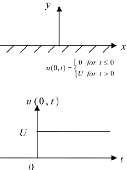
The fluid-mechanics benchmark problem which is referred to as the Stokes’ first problem is equivalent to many branches of engineering and sciences. The situation which is considered is shown in Fig. 1 in the fluid-mechanics texts. The x axis coincides with an infinite long flat plate above which a fluid exists. The

Fig. 1 Definition sketch for Stokes’ first problem (ref. [18] pp. 225)

plate and the fluid are both at rest initially. Suddenly, the plate is jolted into motion in its own plane with a constant velocity.

To simulate the problem, we consider that a semi-infinite region of stationary fluid which is fixed by a rigid plane (at y = 0) is suddenly given a constant velocity U in its own plane and then keeps at that speed. The fluid is brought into motion through the action of viscous stress at the plate. The velocity distribution is governed by the diffusion equation

2 2 u _v u t y ∂ ∂ = ∂ ∂ (1)

where u is velocity and v is kinematic viscosity.

The initial and boundary conditions are shown as below. 0 0 (0, ) 0 ( , ) for t u t U for t u y t finite ≤ ⎧ = ⎨ _> ⎩ = (2) The analytical solution of the Stokes’ first problem is

given by [18] ( , ) 1 erf 2 u y t y U vt ⎛ ⎞ = − _{⎜ ⎟} ⎝ ⎠ (3)

where erf( ) is the error function.

2.2 Stokes’ Second Problem

The Stokes’ second problem differs from the Stokes’ first problem only in the condition that the boundary condition at y = 0 is induced by linear harmonic oscillations with frequency, n, in time instead of suddenly accelerating to move. The phenomenon of the flow and the nature of the boundary condition are indicatedinFig.2. Sincethegeometryisthesame as

x

Fig. 2 Definition sketch for Stokes’ second problem (ref. [18] pp. 229)

that of the previous section and the motion is again in the plane of the boundary itself, the differential equation to be satisfied by u(y, t) will be the same. So the velocity distribution is governed by the same diffusion equation 2 2 u _v u t y ∂ ₌ ∂ ∂ ∂ (4)

The initial and boundary conditions are shown as below. 0 for 0 (0, ) cos( ) for 0 ( , ) finite t u t U nt t u y t ≤ ⎧ = ⎨ _> ⎩ = (5) The analytical solution of the Stokes’ second problem

is given by [18] ( , ) exp cos 2 2 u y t n n y nt y U v v ⎛ ⎞ ⎛ ⎞ = ⎜_⎜− ⎟_⎟ ⎜_⎜ − ⎟_⎟ ⎝ ⎠ ⎝ ⎠ (6)

where n is the oscillating frequency. From the above assumptions and definitions, the Stokes’ first and second problems can be represented by the diffusion equation. So we can apply the unsteady MFS based on the diffusion fundamental solution to simulate these phenomena, which had been proposed by Young et al. [16,17]

3. NUMERICAL METHOD

First of all, we derive the fundamental solution of the linear diffusion equation. The fundamental solution of the linear diffusion equation is governed by

G x t( , ; , ) t ∂ ξ τ ∂ r r = ∇v G x t2 ( , ; , )r ξ τ + δ − ξ δ − τr (xr r) (t ) (7)

in which xr represents the location of the field points and ξr gives the location of the source points. t and τ are the time of the field and source points respectively. By taking Fourier transform with respect to xr and Laplace transform for t and then inversing the transforms of Eq. (7), the free space Green’s function or the fundamental solution of the diffusion equation can be obtained as 2 | | 4 ( ) / 2 e ( , ; , ) ( ) [4 ( )] x v t d G x t H t v t − ξ − − τ ξ τ = − τ π − τ r r r r ₍₈₎

where d is the spatial dimension number and takes 1 in this study, and H( ) is the Heaviside step function.

Since the diffusion fundamental solution satisfies the homogeneous diffusion equation, the solution can be assumed as a linear combination of the fundamental solution of the diffusion operator. According to the method of unsteady fundamental solutions proposed by Young et al. [16,17], the numerical solutions of the diffusion equation will be of the following form.

1 ( , ) i b ( , , , ) N N j j j j u x t G x t + = =

∑

where Ni and Nb are the numbers of initial and boundary

source points and αj are the undetermined coefficients

which can be determined by the method of collocation through the satisfactions of the initial and boundary conditions. The distributions of the field points and the source points are shown in Fig. 3 for the unidirectional domain of this study. The consideration of the issue of unknown source positions can be found in references of Fairweather et al. [10,15]. In Fig. 3, the field points are placed at the boundary portion at t = (n + 1)∆t and in the interior domain at t = (n)∆t. The source points are placed in the same position but at different time levels. By collocating these field points and using Eqs. (2), (5) of the initial and boundary conditions, a linear matrix system can be formed as following

Fig. 3 Schematic diagram for the locations of source points and field points on the space-time domain t (n−0.5)∆t (n+0.5)∆t y ( )n t∆ ( 1)n+ ∆t Field Point Source Point ⎩ ⎨ ⎧ > ≤ = 0 ) cos( 0 0 ) , 0 ( for t nt U for t t u

x

t

[A_ij]{ } { }α =_j b_i (10) where 2 | | 4 ( ) 1/ 2 if [4 ( )] 0 if i j i j x v t i j i j ij i j e _{t τ} v t A t τ −ξ − −τ ⎧ ⎪ > ⎪⎪ _{π − τ} = ⎨ ⎪ ⎪ ≤ ⎪⎩ r r (11)

The matrix {bi} is the combination of initial and

boundary conditions. After inverting the matrix system, the coefficients αj can be solved and the

function values inside the time-space box can thus be obtained by Eq. (9). This procedure can be repeated until either the terminating time or steady state solution is achieved.

4. RESULTS AND DISCUSSIONS

The proposed numerical scheme based on the diffusion fundamental solution is validated by comparing the results obtained by the analytical solutions for the Stokes’ first and second problems which are the benchmarks in the realm of fluid dynamics. And the maximum absolute errors for different time increments and different numbers of node points have been analyzed. The effectiveness of the unsteady MFS is verified by solving these two Stokes’ problems and the results obtained are discussed in the following sections.

4.1 Stokes’ First Problem

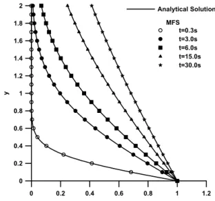
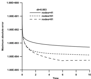
In the fluid-mechanics context the situation which is being considered is shown in Fig. 1. The comparison between the MFS based on the diffusion fundamental solution and the analytical solution of the u-distribution versus the wall distance for different times is depicted in Fig. 4 for v = 0.1. It is clearly found that the numerical results are in good agreement with the analytical solutions. The transient process can be simulated very well by comparing with the time-dependent analytical solution. The variations clearly demonstrate the physics underlying the Stokes’ first problem phenomena. In other words, the diffusion fundamental solution is a time-dependent function, which is capable to capture the transient process. The disturbance caused by the impulsive motion of the boundary diffuses into the fluid as a function of the time from the initiation of the motion progresses as expected. Moreover, Fig. 5 shows the time evolution of u at a point y = 0.5 from the wall. The value of u is asymptotically closed to 1 as the time grows. Figures 6 and 7 depict the maximum absolute errors for different time increments and different node points, respectively. The results reveal that generally the more node points and smaller time

0 0.2 0.4 0.6 0.8 1 1.2 u 0 0.2 0.4 0.6 0.8 1 1.2 1.4 1.6 1.8 2 y MFS t=0.3s t=3.0s t=6.0s t=15.0s t=30.0s Analytical Solution

Fig. 4 Comparison of u-distribution at different time levels for Stokes’ first problem

0.01 0.1 1 10 100 1000 10000 Time -0.2 0 0.2 0.4 0.6 0.8 1 u ( y= 0 .5 ) Analytical Solution MFS

Fig. 5 Comparison for Stokes’ first problem time evolution of u at y = 0.5 0 2 4 6 8 10 Time 1.00E-005 1.00E-004 1.00E-003 1.00E-002 1.00E-001 1.00E+000 M axi m u m ab so lu te err o r nodes=61 dt=0.001 dt=0.005 dt=0.01

Fig. 6 Time evolution history of maximum absolute error for different time increment

0 2 4 6 8 10 Time 1.00E-005 1.00E-004 1.00E-003 1.00E-002 1.00E-001 1.00E+000 Maxim u m absolute e rr o r dt=0.003 nodes=41 nodes=61 nodes=81

Fig. 7 Time evolution history of maximum absolute error for different numbers of points

increments are used the better results are obtained as expected, after careful checking the maximum absolute errors at each field point and different time increment.

4.2 Stokes’ Second Problem

The Stokes’ second problem differs from the Stokes’ first problem only in the boundary condition. The oscillatory nature of the flow generates depressive harmonic waves in the velocity field. The comparison of u-distribution versus the wall distance at different time levels for the Stokes’ second problem for v = 0.1 is depicted in Fig. 8. The boundary is oscillating in time, it is expected that the fluid will also oscillate in the y direction in time with the specific frequency. Since the diffusion fundamental solution is a time-dependent function, it is able to capture the transient process by this unsteady MFS technique. The salient features of velocity variations also clearly demonstrate the physics underlying the Stokes’ second problem process. The time evolutions of u at y = 0.5 and y = 1 from the oscillating wall are displayed in Figs. 9 and 10, respectively with the comparisons of analytical solutions. The amplitude is conspicuously decreased from the oscillating wall. The maximum absolute errors in the semi-infinite domain for different time increments are displayed in Fig. 11. On the other hand, Fig. 12 depicts the maximum absolute errors with different node points. The periodic cycles of the numerical errors show the reasonable and stable results for our numerical scheme. As expected, smaller time increment and more node points always give better results. Although these diffusive waves decay rapidly, the maximum absolute errors still can be controlled under very stable condition by this unsteady MFS numerical scheme.

5. CONCLUSIONS

The Stokes’ first and second problems are solved using the unsteady MFS based on the diffusion

-1.2 -0.8 -0.4 0 0.4 0.8 1.2 u 0 1 2 3 4 5 y MFS t=20s t=40s t=60s t=80s t=100s Analytical Solution

Fig. 8 Comparison of u-distribution at different time levels for Stokes’ second problem

0 20 40 60 80 100 Time -0.40 -0.20 0.00 0.20 0.40 u ( y=0 .5 ) Analytical Solution MFS

Fig. 9 Comparison for Stokes’ second problem time evolution of u at y = 0.5 0 20 40 60 80 100 Time -0.15 -0.10 -0.05 0.00 0.05 0.10 0.15 u (y =1) Analytical Solution MFS

Fig. 10 Comparison for Stokes’ second problem time evolution of u at y = 1

0 20 40 60 80 100 Time 1.00E-006 1.00E-005 1.00E-004 1.00E-003 Ma xim u m a b so lu te e rr o r nodes=41 dt=0.2 dt=0.1 dt=0.05

Fig. 11 Time evolution history of maximum absolute error for different time increment

0 20 40 60 80 100 Time 1.00E-008 1.00E-007 1.00E-006 1.00E-005 1.00E-004 1.00E-003 1.00E-002 Maxi mum absol u te e rr o r dt=0.05 nodes=21 nodes=41 nodes=61

Fig. 12 Time evolution history of maximum absolute error for different numbers of points

fundamental solution directly without using any kind of time transformation or discretization. For an unsteady and semi-infinite domain problem, the unsteady MFS is a very powerful and efficient method to deal with. The problem can be figured out precisely and quickly using this novel method. The independent variable for time was treated as one of the solution domains in the unsteady fundamental solutions. This space-time unification concept has made us possible to take the advantages of the method of unsteady fundamental solutions to obtain direct numerical solutions of diffusion equation without transformation or discretization for the time domain. By properly locating the source points and the field points at every time level, the solution is advanced in time to get results until the system reaches the steady state conditions. The excellent agreement of the present results with the analytical solutions indicates the effectiveness of the present method to directly solve the Stokes’ first and second problems by the unsteady MFS based on the diffusion fundamental solution.

ACKNOWLEDGEMENT

The National Science Council of Taiwan is gratefully acknowledged for providing financial supports to carry out the present work under the grant no. NSC 93-2611- E-002-001.

REFERENCES

1. Zhu, S. P., “Solving transient diffusion problems: time-dependent fundamental solution approaches versus LTDRM approaches,” Engng. Anal. Bound. Elem., Vol. 21, pp. 87−90 (1998).

2. Zhu, S. P., Liu, H. W., and Lu, X. P., “A combination ofLTDRMandATPSinsolvingdiffusion problems,” Engng. Anal. Bound. Elem., Vol. 21, pp. 285−289 (1998).

3. Bulgakov, V., Sarler, B., and Kuhn, G., “Iterative solution of systems of equations in the dual reciprocity boundary element method for the diffusion equation,” Int. J. Numer. Meth. Engng., Vol. 43, pp. 713−732 (1998).

4. Zerroukat, M., “A boundary element scheme for diffusion problems using compactly supported radial basis functions,” Engng. Anal. Bound. Elem., Vol. 23, pp. 201−209 (1999).

5. Sutradhar, A., Paulino, G. H., and Gray, L. J., “Transient heat conduction in homogeneous and non-homogeneous materials by the Laplace transform Galerkin boundary element method,” Engng. Anal. Bound. Elem., Vol. 26, pp. 119−132 (2002).

6. Bialecki, R. A., Jurgas, P., and Kuhn, G., “Dual reciprocity BEM without matrix inversion for transient heat conduction,” Engng. Anal. Bound. Elem., Vol. 26, pp. 227−236 (2002).

7. Tsai, C. C., “Meshless numerical methods and their engineering applications,” Ph.D. Dissertation, Department of Civil Engineering, National Taiwan University, Taipei, Taiwan (2002).

8. Golberg, M. A., “The method of fundamental solutions for Poisson’s equation,” Engng. Anal. Bound. Elem., Vol. 16, pp. 205−213 (1995).

9. Golberg, M. A. and Chen, C. S., The method of fundamental solutions for potential, Helmholtz and diffusion problems, Boundary Integral Methods: Numerical and Mathematical Aspects, Golberg, M. A., Ed., Southampton, Boston, Computational Mechanics Publications (1999).

10. Fairweather, G. and Karageorghis, A., “The method of fundamental solutions for elliptic boundary value problems,” Adv. Comput. Math., Vol. 9, pp. 69−95 (1998).

11. Poullikkas, A., Karageorghis, A., and Grorgiou, G., “Methods of fundamental solutions for harmonic and biharmonic boundary value problems,” Comput. Mech., Vol. 21, pp. 416−423 (1998).

12. Poullikkas, A., Karageorghis, A., and Grorgiou, G., “The method of fundamental solutions for inhomogeneous elliptic problems,” Comput. Mech., Vol. 22, pp. 100−107 (1998).

13. Chen, C. S., Golberg, M. A., and Hon, Y. C., “The method of fundamental solutions and quasi-Monte- Carlo method for diffusion equations,” Int. J. Numer. Meth. Engng., Vol. 43, pp. 1421−1435 (1998). 14. Balakrishnan, K. and Ramachandran, P. A., “The

methodoffundamentalsolutionsforlineardiffusion- reaction equations,” Math. Comput. Modeling, Vol. 31, No. 2-3, pp. 221−237 (2000).

15. Fairweather, G., Karageorghis, A., and Martin, P. A., “The method of fundamental solutions for scattering and radiation problems,” Engng. Anal. Bound. Elem., Vol. 27, pp. 759−769 (2003).

16. Young, D. L., Tsai, C. C., and Fan, C. M., “Direct

approach to solve nonhomogeneous diffusion problems using fundamental solutions and dual reciprocity methods,” J. Chin. Inst. Engng., Vol. 27, pp. 597−609 (2004).

17. Young,D.L.,Tsai,C.C.,Murugesan,K.,Fan,C.M., and Chen, C. W., “Time-dependent fundamental solution for homogeneous diffusion problem,” Engng. Anal. Bound. Elem., Vol. 28, pp. 1463−1473 (2004).

18. Currie, I. G., Fundamental Mechanics of Fluids, 2nd Ed., McGraw-Hill, Boston (1993).

(Manuscript received September 20, 2004, Accepted for publication January 25, 2005.)