Dynamic output feedback control of nonlinear singularly perturbed systems

~ ) Pergamon

J. Franklin Inst. Vol. 333B, No. 6, pp. 947 973, 1996 Copyright © 1996 The Franklin Institute P I h S0016-0032(96)00042-7 Published by Elsevier Science Ltd Printed in Great Britain 00164)032/96 $15.00+0.00

Dynamic Output Feedback Control of Nonlinear

Singula@ Perturbed Systems

b y S H I N G - T A I P A N

Department o f Control Engineering, National Chiao Tung University, 1001 Ta Hsueh Road, Hsinchu, Taiwan 300, R.O.C.

F E N G - H S I A G H S I A O

Department o f Electrical Engineering , Chang Guny College o f Medicine and

Technology, 259 Wen-Hwa 1st Road, Kwei-San Taoyuan Shian, Taiwan 333, R.O.C. a n d C H I N G - C H E N G T E N G

Department o f Control Engineering, National Chiao Tun9 University, 1001 Ta Hsueh Road, Hsinchu, Taiwan 300, R.O.C.

(Received 17 January 1996; acccepted 15 March 1996)

ABSTRACT : In this paper, the stabilization problem of two classes of nonlinear singularly perturbed systems via dynamic output feedback is investigated. First, we consider the nonlinear singularly perturbed systems in which the nonlinearities are continuously differentiable. The theoretical result demonstrates that, using the factorization approach, the dynamic output feedback controller designed for the reduced-order model of the linearized system is a stabilizing compensator for the original nonlinear singularly perturbed system, provided that e is sufficiently small. Second, the nonlinear singularly perturbed systems in which the nonlinearities are not necessarily continuously differentiable but satisfy the global Lipschtz condition are examined. Combining the dynamic output feedback controller that stabilizes the reduced-order model of the linear part of the nonlinear singularly perturbed system with the quasi-stability result of Persidskii, a two-step compensating scheme is proposed to stabilize the original nonlinear singularly perturbed system under con- siderationfor a sufficiently small e. Copyright © 1996 Published by Elsevier Science Ltd

L Introduction

Most physical systems contain some small parameters such as small time constants, masses, capacitances, etc. These small parameters increase the order of dynamic systems and then complicate the system analysis. Furthermore, they introduce the multi-time- scale property such that these systems simultaneously possess b o t h slow states and fast states. Coupling of these states with each other makes the system analysis m u c h more

948 S.-T. Pan et al.

complex, and hence convenient methods to check stability have long been sought. Fortunately, singularly perturbed models for these systems give us a powerful tool for order reduction and separation of time scales. This singular perturbation approach, arising from an attempt to approximate a high-order system with another one of lower order, has proven to be a successful analytical tool that exploits directly the separation of system time scales, made explicit by the small singular perturbation parameter e. When e is small enough, approximations are obtained from the reduced-order models in separate time scales (1).

Singularly perturbed systems have been studied extensively in recent years; see, for example, Kokotovic et al. (2) and references therein. This is due not only to theoretical interest, but also to the relevance of this topic to control engineering applications. Indeed, the singular perturbation approach has been proven to be an effective tool for system analysis and control design (3). A fundamental feature of such a control theory is decomposition of the feedback design problem into two design subproblems for the slow and fast dynamics. The two designs are then combined to give a design for the full-order system (4). Moreover, if the fast subsystem is already stable, the only work we need to do is to design the stabilizing feedback control in the slow subsystem (i.e. reduced-order model). The stabilizing feedback control designed for the reduced-order model can stabilize the full-order system, provided that e is sufficiently small.

The dynamic output feedback control problem of singularly perturbed systems has been addressed in many works. However, these contributions focused mainly on linear singularly perturbed systems; see, for example (5-8). In this work, the stabilization problem is investigated for two classes of nonlinear singularly perturbed systems via dynamic output feedback. First, we examine the nonlinear singularly perturbed systems in which the nonlinearities are continuously differentiable. Using the factorization approach, the dynamic output feedback controller is designed for the reduced-order model of the linearized system of the nonlinear singularly perturbed system. The theoretical result demonstrates that the above dynamic output feedback controller can stabilize the linearized system and then the original nonlinear singularly perturbed system as well, provided that e is sufficiently small. Second, the nonlinear singularly perturbed systems in which the nonlinearities are not necessarily continuously differ- entiable but satisfy the global Lipschtz condition are investigated. Combining the dynamic output feedback controller that stabilizes the reduced-order model of the linear part of the nonlinear singularly perturbed system with the quasi-stability result of Persidskii, a two-step compensating scheme is proposed to stabilize the original nonlinear singularly perturbed system under consideration, provided that e is sufficiently small.

This paper is organized as follows. In Section II, the factorization approach for designing the dynamic output feedback controllers in linear systems is introduced. In Section III, we consider a class of nonlinear singularly perturbed systems in which the nonlinearities are continuously differentiable. The factorization approach is used to design the dynamic output feedback controller for the reduced-order model of the linearized system such that the original nonlinear singularly perturbed systems is asymp- totically stable at the origin. The class of nonlinear singularly perturbed systems in which the nonlinearities are not necessarily continuously differentiable but satisfy the global Lipschtz condition is examined in Section IV. A two-step compensating scheme

Nonlinear Sinyularly Perturbed Systems 949

rp + up

--+

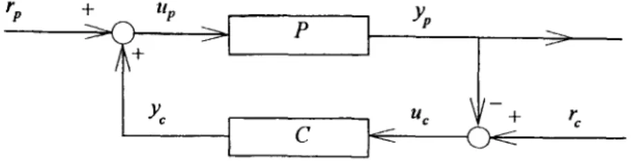
FIG. 1. One-parameter compensating scheme.

r

is proposed to stabilize the original nonlinear singularly perturbed system under con- sideration. Two illustrative examples are given in Section V. Finally, conclusions are provided in Section VI.

II. Factorization Approach

The factorization approach for designing the dynamic output feedback controllers in linear systems is reviewed in this section.

Consider the feedback system shown in Fig. 1: P represents the plant and C the compensator; rp and rc the external inputs; Up and uc the inputs to the plant and compensator, respectively; yp and Yc the output of the plant and compensator, respec- tively.

Assume P is proper and has a state-space realization:

Clearly we have

Defining

= Apx + Bpup,

yp = CpX + EpUp. O)

P(s) = Cp(sI- Ap)- l Bp + Ep.

r'lr,, I rc]

for the feedback connection o f Fig. 1, we can get

u =- H ( P , C)r,

where

= ~ (I+PC) ' - - P ( I + C P ) - I ]

H(P, C) [_C(I+PC) ' ( I + C P ) - ' ]" (2)

If the compensator C is so chosen that d e t ( I + PC) ~ 0 and H(P, C) ~ M(S(s))t, then C stabilizes P ( i n p u ~ o u t p u t stability). Assume that the pairs (Ap, Bp) and (Ap, Cp) are ~The set of matrices whose elements are proper stable rational functions in s with real coefficients.

950 S.-T. Pan et al.

stabilizable and detectable, respectively; the following theorem gives parametrization o f the set of the stabilizing compensators C for P.

Theorem I (9)

Suppose that for the system (1) P e M ( R ( s ) ) ? and (Np, Dp), (/)p, Np) are any right

coprime factorization and left coprime factorization of P, respectively. Select matrices

Up, Vp, 0p, ITp in M(S(s)) such that

UpNp + VpD~ = I (3)

NpUp + DpVp = I. (4)

Denote S(P) the set of all Cs in M ( R ( s ) ) that stabilize P, i.e. the set of all Cs in M(R(s))

such that H(P, C) ~ M(S(s)). Then

S(p) = { ( Vp - RNp) ~ (Up + R/)p): R e M(S(s)), det(Vp - RhTp) 4= 0}

= { ( O p + O p S ) ( 1 2 p - N p S ) - l : S 6 M ( S ( s ) ) , d e t ( l Y p - N p S ) ~ 0}. (5) Note that all the matrices in (3)-(4) can be calculated by the following:

No

ap

Up

V.

0.

g

in which K and F are Hurwitz.

To discuss the internal stability of the feedback system in Fig. 1, the compensator C is realized in state-space form as

:to = Acx~ + Bout,

y< = Ccx~ + E~uc (7)

with the transfer function

= C p ( s I - (Ap - - F C p ) ) - ' ( B p --FEp) +Ep, = I - C p ( s I - (Ap

--FCp)) -IF,

= ( C p - E p K ) ( s I - ( A p - B p K ) ) - ' B p + E p , = I - - K(sI-- (Ap - B p K ) ) - 'Bp, = X ( s I - (Ap - FCp))- ' F, = I + K ( s I - (Ap - FCp)) -~ (Bp - VEp), = K(sI-- (Ap -- S p K ) ) - 'F, = I + (Cp - E p K ) ( s I - (Ap - B p K ) ) - ' r , (6)

properly chosen such that both Ap--BpK and Ap--FCp are

H<(s) ~- C c ( s I - Ac)- ' Bc + E<.

The following theorem states the relationship between internal stability and input- output stability for the feedback system of Fig, 1.

Nonlinear Singularly Perturbed Systems 951

Theorem H (9)

Suppose that the two triples (Ap,

detectable and that

Bp, Cp) and (Ac, Be, Cc) are both stabilizable and

d e t ( I + / / ~ ( o o ) P ( o o ) ) = d e t ( I + EcEp) # O.

Under these conditions, the closed-loop system of Fig. 1 is asymptotically stable if

H(P, C) ~ M(S(s)). •

In the following sections, the factorization approach is applied to stabilize two different classes o f nonlinear singularly perturbed systems.

Ill. Dynamic Output Feedback Controller

Consider the following nonlinear singularly perturbed system: -*l = f l (Xl ,x2, u)

&X'2 = f2 (x,, x2, u)

y = g(x~, x2), (8)

where the nonlinear functions f~, fz and g are continuously differentiable and f~(0,0,0) = 0,f2(0, 0, 0) = 0 and g(0,0) = 0.

In this section, dynamic output feedback controllers are designed such that they can asymptotically stabilize the nonlinear singularly perturbed system (8) at the origin. Define = All X ~ , `412 = OXl [Xl=O,x2=O,u=o ~X2 xl = `421 ~ , A22 = O X l Ix I = 0 , x 2 = 0 , u = 0 ~ X 2 x I O X l Ix I = 0 , x 2 = 0

Therefore, the linearized system o f (8) reads

= 0,x 2 = 0 ,u = 0 = O,x2 = O , u = O B 1

--:0~

-fi

O U Ix I =0,X2 =0,~d=0 B2 = Of 2 ~ U XI = 0 , X 2 = 0 , [ / = 0 ' (9)

Jell = .41 lXll-{-`412X2I+ BlUl,

&~2: = A21Xll+`422X21-{-B2Ul,

Yt = ClXlt+ C2X2l. (10)

The matrix

.422

is assumed here to be nonsingular and Hurwitz. Furthermore, the reduced-order model o f system (10) can be obtained by setting e = 0 in Eq. (10), i.e.

"~ll ~----

All-~llq-Al2-~2l"k Blal,

0 = A21.~ll+A22-~21"~-B2171h

(11) (12)

952 S . - T . P a n et al.

0

-~,

u t ..~[ .~u = Ao~ u + Bo~ t

Y t

d~ ~- ~ Y-/____~

Xl___~/q-

C0

0~..._~/

g

1did

2 >

0

. . . i FIG. 2. Dynamic output feedback scheme for the reduced-order model (15).

Y l = C l X l l - ~ - C 2 X 2 l .

Since A22 is nonsingular, we can get, from (12), that

YC21 = -- A221AzlYcII-- A221B2(II.

Substituting (14) into

(1 1) and (13)

yields

x l l = A o ~ l t + Bo~t, f l = C o 2 ~ l + Eo~l, in which (13)

(14)

(15)

xta = AaXta + Basra

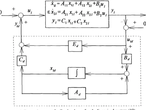
Yld = C d ' ~ l d - ~ EdUld" (17) It will be shown that the dynamic output feedback controller (17) can also stabilize the

Ao = A l l - A 1 2 A y 2 1 A 2 1 , Bo = B l - A L 2 A ~ 2 1 B 2 ,

Co = C 1 - - C 2 A 2 2 1 A 2 1 , Eo = - - C z A z 2 1 B 2 . (16) The system (15) is generally referred to as the reduced-order model o f the linearized system (1 0). Suppose that the dynamic output feedback controller, which stabilizes the reduced-order model (1 5) under the feedback interconnection as depicted in Fig. 2, can be obtained from Theorem I and is realized as

Nonlinear Singularly Perturbed Systems

953

+

Jcu=Allxu+Al2X2t+B~uj

ut

~:.I ~X~t=A~iX, t+A22x2i+B:u, Y,

)

I

I+

I Yt=qxlt+C2x2t

-I

t

~

(

( ) <

+ +

>[

I

+

///d

+

0

FIG. 3. Dynamic output feedback scheme for the linearized system (10).

linearized system (10) and then the original nonlinear singularly perturbed system (8) as well, provided that the singular perturbation parameter ~ is sufficiently small.

Lemma 1

Suppose that the two triples

(Ao, Bo, Co)

of (15) and

(Ad, Bd, Cd)

of (17) are both stabilizable and detectable and assume that

(Aa, Ba, Cu, Ed)

of (17) is a stabilizing compensator for (A0, B0, Co, E0). Let Ed be chosen such that the matrix

(I+EdEo)

exists and

B2Ed

= 0 or

EaC2

= 0. Then, for a sufficiently small e, the linearized system (10) is stabilized by the dynamic output feedback controller (17) under the feedback scheme shown in Fig. 3.

Proof'.

From Fig. 2 it can be seen that

o ro,1,

~,.J L o

B.JLat~,J

ov,,l+[oo olro, l,

Y,.J L o

CdJLX,dJ

EdJLa,d

[a~;]= [71

1l[37' 1

OJL:ta/

954

S.-T. Pan

et al.

][~_1,]

xlaJ k(-Ba+BaEo(I+EaEo)-lEa)Co

Aa-BaEo(I+EaEo)-ICaJkxlaJ"

(18) Since the two triples (Ao, Bo, Co) of (15) and

(Aa, Be, Cd)

of (17) are both stabilizable and detectable, the system (18) is, according to Theorem II, asymptotically stable. Hence the matrix

= r

Ao-Bo(I+EaEo)-'EaCo

Bo(I+EaEo)-'Ca

1 (19)

Ho - m(- Ba+ BaEo(I+ EdEo)-' Ea)Co Aa- BaEo(I+ EaEo)-'CaJ

in (18) is Hurwitz.

Moreover, the dynamic output feedback controller (17), by changing the notations of variables, is rewritten here as:

2~a = Aaxtd + Bauta,

Yta = Caxta + Eauta.

From Fig. 3 it can be seen that

[ 21t ] [AII-B1EaC1

BICa

X,a / = ]

-BaC1

Aa

8-~21J LA21 - B 2 g d C l B2Ca

A,2 Bl C21[x,, 1

A22

--B2EdC2

J [. X2/J

If the parameter Ea is chosen such that

B2Ea

= 0 or

EaC2

= 0, then (20) becomes

[A,,-B, Eacl B,c

~,a]= / -~,c,

Aa

~22t J L A 21

-- B2 EaCI

B2 Ca

A , z - B, EdC2 ][ Xl, ]

- B ~ q i x , a [ A22 [_x21J (20) (21) o r

I

AII-B1EaCI

BiCa Alz-BaEaC2

972t

8 g

xll ]

%j

(22)

Moreover, the system (21) can be rewritten in a more compact form as the following:

N1 : N2 ...

N3 !

L E ~ /

x,, 1

Xld] ,

X2l 3

(23) where

Nonlinear Singularly Perturbed Systems

= F A I I - - B ' E d C I B l C d l , V A I 2 - - B I E d C 2 1

N,

L

- B d C , A d J N2 = l - B . c : j'

N3 = [A21 -B2EuC1 BzCa], N4 = A22.

Applying the following transformation to (21) (2):

i.e.

I Xll

X2l

2 1 gPd

...

I - c L a P d

in which L d and Pd satisfy

I__ePdL d " _ e p d L d I

~.2 ] ,

xll 1

Xld ] '

X2I .J 955 (24) (25) No = NI - - N 2 N 4 IN3 = F A l l - - B I E d C l

L

- B d C I

=F

LU~o U~J

B 1 C d l _ _ [ - A I 2 - - B I E d C 2 1 l N ~ = A , , - B I E a C , - ( A I 2 - - B , EdCz)Ay21(A21-- B2EaC,), N~ = B, Cd-- (A12 --BIEdC2)A221B2Cd, B2 Cd] (28) with where N 3 -- N 4 L d + eLaN ~ - 8LdN 2 L d = 0, e(N, - N z L d ) P a - Pd(N4 + eLdN2) + N2 = 0, (26) the closed-loop system (21), or equivalently (23), can then be converted into a decoupled form as the following:

2

(27)

956 S.-T. Pan et al.

N 3 = - BaC, + BdC2A22 ~

(A2,

-- B2EaC1), N 4 = Aa+BaC2A221BzCa.

Based on (16) and the fact that

( I + M N ) - - 1 = I - M ( I + N M ) - 1N,

we have

( I + EdEo)-' = (I-- EaCaA22' B2) 1 = I + EdC2(I--Azz' BzEdC2) 1A~2' B2 = I+EdCzA22' B2 ('." B2EaC2 = 0).

After lengthy manipulations, it can be shown that No is identical to H0 (in (19)) and thus Hurwitz. Since No and N4 (i.e. A=) are both Hurwitz, the closed-loop system (27), or equivalently (21), is hence asymptotically stable for a sufficiently small e. This

completes the proof. •

R e m a r k 1

If the matrix Ed can not be properly chosen such that BzE a = 0 or EdC2 = 0, then the following conditions (2) can be used to guarantee the result of Lemma 1:

(i) The pair ( A 2 2 , B2) is weakly controllablet; (ii) The pair (C2, A22) is weakly observable%

The following theorem demonstrates that the dynamic output feedback controller, designed for the reduced-order model (15), can stabilize the original nonlinear singu- larly perturbed system (8).

Theorem I I I

Suppose that all the assumptions in L e m m a 1 are available. Then, the pair (Aa, Ba, Ca, Ea) of (17), which is designed for the reduced-order model (15), is a sta- bilizing compensator for the original nonlinear singularly perturbed system (8) under the feedback configuration of Fig. 4, provided that e is sufficiently small.

Proof'. The dynamic output feedback controller (17), by changing the notations of variables, is rewritten here as

"~d = AdXd "}- BdUd,

Yd = CdXd + EdUd. (29)

F r o m Fig. 4 we have

-~1 = f I ( X I , X 2 , U ) ,

xa = AdXd-- Bag(x1, x2),

t The weak controllability and weak observability of the fast eigenvalues (i.e. the eigenvalues of A22) mean that they will not be affected by more than O(e) through output feedback.

0

Nonlinear Singularly P e r t u r b e d S y s t e m s

+

]

~,--Y,(x,, x2..)

> r ~ u ~ l ~X2 = f 2 ( x , , x2 ,U) Y

,Ya~

+_~.

I

Y=

g(xl'x2)

-i

. . .

~"

I )

A, I

+

0

<5 . . . . I ra I I I I i i i d i i

)

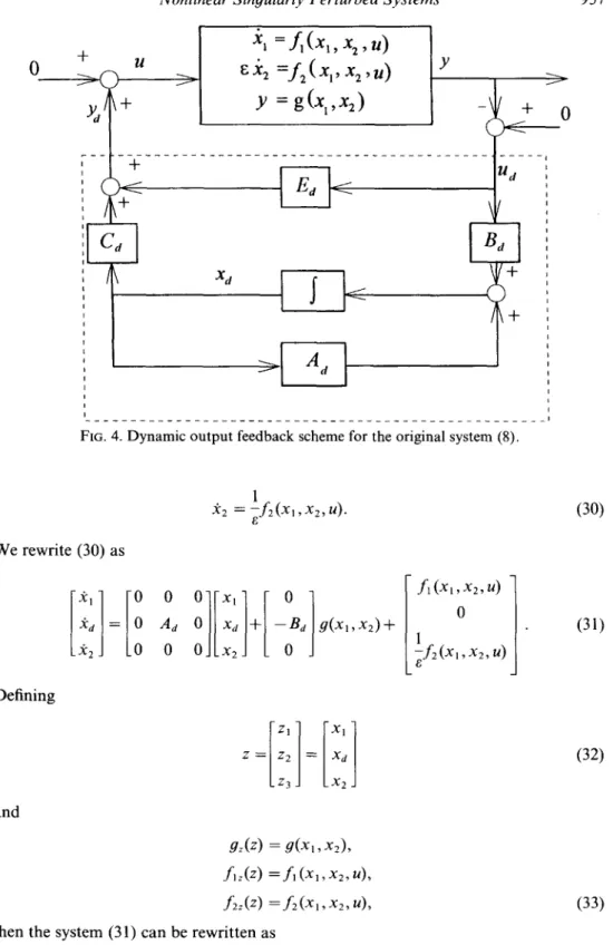
+ 957

FIG. 4. Dynamic output feedback scheme for the original system (8).

We rewrite (30) as 1

~

= -A(x,, x2, u).

₈ Defining and Xd = Aa 0 Xd + a x2 0 OJLx2J L

I A(x~,x2,u) ]

0 9 ( x l , x2) + 1 -f2 (x l, x2, u) 8

[z I i x,1

Z Z 2 ~- X d Z3 X2

gz(z) = g(xl, xO,

f,z(z) =A (x,, x2, u),

U 2 z ( Z ) = f 2 ( X l , X 2 , U ) ,

then the system (31) can be rewritten as

(30)

(31)

(32)

958 S.-T. Pan et al.

e = Z(z), (34)

where

i ,,z,l 1!o! 1o / F :z,1

(35)

In order to analyze the stability o f system (34), we calculate the Jacobian matrix of

Z(z) at z -- 0: 63Z, 63z, ~-zz ~ = o 63Z2 63z~ 63Z3 63z, 63Zj OZ, &2 &3 63Z2 OZ2 63Z 2 63Z 3 63Z3 63Z3 &2 &3 _z=O

(36) with 63Z1 z=0 _{63zl = A,l - B , E a C , , 63ZI63z2 z=0 = Bl}

_Cd,

63Z1 z=0 _{= A 1 2 - B , E a C 2 ,}

63Z2 ~= o

63Z2

63Z2 = - B a C , , = A d , = - - B a C 2 , 632, z=0 63Z2 OZ3 z=0

63Z36321 z=0 = (A21

--B2EaC,)/3

' 63Z36322 z=O --

B2Cd/3

' 63Z36323 z=O - A22/3

Obviously the matrix in (36) is identical to the system matrix o f (22). It is noted that since the closed-loop system (27), or equivalently system (22), is asymptotically stable for a sufficiently small/3, the Jacobian matrix of Z(z) at z = 0 is Hurwitz, provided that /3 is sufficiently small. Hence, we can see that if/3 is small enough, then the dynamic output feedback controller (29) can stabilize the original nonlinear singularly perturbed system (8) under the feedback configuration o f Fig. 4. This completes the proof. •

Remark 2

The special cases

~, = f , ( x , , x 2 , u ) , /3~2 = f 2 ( x , , x 2 ) ,

y = g ( x , , x 2 ) , (37)

Nonlinear Singularly Perturbed Systems 959

)¢1 = f l (Xl, X2, U), e-t2 = f z ( x l , x2, u),

y = g ( x , )

(38)

will lead to B2 = 0 or C2 = 0, respectively. Hence, the assumption B2Ea = 0 or EaC2 = 0

in L e m m a 1 is always satisfied for any Ea.

So far, we have considered the nonlinear singularly perturbed system (8) in which the nonlinearities are continuously differentiable. The class of nonlinear singularly perturbed systems in which the nonlinearities are not necessarily continuously differ- entiable but satisfy the global Lipschtz condition is examined in the next section.

IV. Two-step Compensating

Scheme

Consider the following nonlinear singularly perturbed systemt:

Jq = A1 lxl +A 12x2 +fl (xl, x2) + B I u,

/;'~2 = A21Xl -t-A22x2

-t-f2(xl,x2)~-B2u,

y = ClXl + C2x2 +9(Xl, x2) (39)

where x~e~", x z E ~ m, u ~ t " , , y ~ l " o . The functions fl: ~n X ~ " - - * ~", f2: ~ " X ~m--+

,~rn, 9: "~nX'-~m---~n°;

All, A12, A21, A22, BI, 02, C1 and C2 are the real matrices of a p p r o p r i a t e dimensions. The system (39) can be rewritten in a m o r e c o m p a c t form as the following: 2 = A x + f ( x ) +Bu y = Cx + 9x (x), (40) where

1

f(x)=[f2(x:__,x2) ], 9x(X)=g(x,,x2). (41)

The following assumptions are m a d e here:

(A1) f(0) -- 0 (i.e.fl(0, 0) = 0 andf2(0, 0) = 0) and 9x(0) = 0 (i.e. 9(0, 0) = 0); (A2) A22 is nonsingular and Hurwitz;

(A3) f and gx satisfy the global Lipschtz condition, i.e. there exist constants kj~ kg

such that

t For the purpose of simplicity, the notations of the matrices in the linear part of system (39) are chosen to be the same as those in the linearized system (10).

960 S.-T. Pan et al.

If(~)-f(q)]l ~

kjll~-~l[,

v ( ~ , o ) e ~ " x ~ m, (42) Ilgx(~)-gx(o)ll ~ kgll~-~ll, X / ( ¢ , ~ ) ~ n x N m. (43) Consider the linear part o f (39):

Xlt = A l l X l t + A12x21+ BlUt, e,22l = A 2 1 x l l + A z 2 x 2 t + B2ul,

Yt = C I X ll ~- C2X2I. (44)

The reduced-order model o f system (44) can be obtained from (15) which is repeated here for convenience:

in which

xlt = Ao~ll+Bot~l,

Yl = CoXllAv EoUl, (45)

Ao = A l l - A I 2 A 2 2 1 A 2 1 , Bo = Bl - A I 2 A 2 2 1 B 2 ,

Co = C 1 - C e A 2 2 1 A 2 1 , Eo = --CzA221B2. (46) The stabilizing controller for the reduced-order model (45), which is described in (17), is also repeated here:

xta = Aa~ta + Bahia,

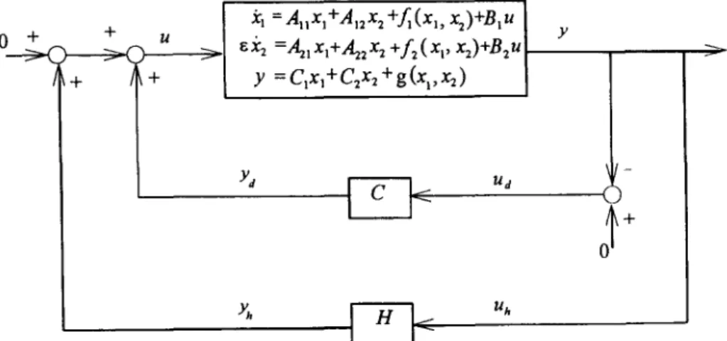
Yta = Ca~ta + Ea~la. (47) In the preceding section we saw that the stabilizing controller (47), which is the realization o f the compensator obtained from Theorem I, also stabilizes the full-order system (44) for a sufficiently small e. The theoretical result demonstrates that combining the dynamic output feedback controller designed for the reduced-order model (45) with the quasi-stability result of Persidskii, a two-step compensating scheme will stabilize the original nonlinear singularly perturbed system (39), provided that e is sufficiently small. The two-step compensating scheme for stabilizing the system (39) is shown in Fig. 5, where C and H are controllers. The controller C is designed for stabilizing the reduced-order model (45) and is realized in (47); however, the variables )zta, )~la and ata are replaced by xa, Ya and ua, respectively. The controller H will be chosen as the following form:

2h = Ahxh +

BhUh

yh = O(llxhlLk),

asllxhll

~ 0, (48)

where A~ is Hurwitz, Bh is a real matrix and k > 1. Moreover, the notation y~ = O(llxhllk), asllxhll ~ 0,

Nonlinear Singularly Perturbed Systems 961

jq =Aux,+A,~x~+f(x,,x~)+Blu :> ~ic~ =&,x,+a~2x ~ + f2( x,, xO+B~u

y = Clxl+ C2x2 + g (xl, x~)

0 + + u Y

Yh

[ " ~ < 2

Ut'

FIG. 5. Two-step compensating scheme for the original nonlinear singularly perturbed system (39).

Ilyhll ~ qllxhll k.

Prior to examination of the stability of the closed-loop system under the two-step compensating scheme, the quasi-stability concept is first introduced.

Consider the nonlinear system which is partitioned into two subsystems of the forms

Jc = X(z, x), (49)

= Z ( z , x).

(50)

Assume that the existence and uniqueness of the solutions of (49) and (50) are guaran- teed and that X(0, 0) = Z(0, 0) = 0. Thus, the origin (z, x) = (0, 0) is an equilibrium point of the complete system. Let y(t) be a continuous vector with compatible dimension and consider the associate system

Yc(t) = X ( y ( t ) , x(t)). (51)

Denote Ox, Oz as the origin (z, x) = (0, 0) of (49) and (50), respectively, and O the origin (z, x) = (0, 0) of the complete system. We say that the origin Ox is quasi-stable for (49) whenever, given any a, there exists a positive b(a) ~< a such that if Ily(0)II < 6 then any solution x(t) of (51) with ]l x(0)I[ ~< 6 has the property that in any time interval 0 ~< t ~< tl, in which Ily(t)rl ~< a, we have Ilx(t)ll < a. Contrapositively, the origin Ox is said to be quasi-unstable for (49) whenever, given any 6, a such that for any y(t) with ily(0) It < 6 and y(t) < a for t ~> 0, then for some solution x(t) of (51) with I[x(0)II ~< 6, we have IIx(t)II ~> a for some t ~> 0. The quasi-stability and quasi-instability for Oz are completely defined analogously.

The relationship between quasi-stability of the subsystems and stability of the com- plete system is stated in the following lemma established by Persidskii.

L e m m a 2 (10)

962 S.-T. Pan et al.

for the complete system. If Ox or Oz is quasi-unstable for the corresponding subsystem, O is then unstable for the complete system.

A type of quasi-stable systems is given in the following lemma.

L e m m a 3 (10) For the system

2 = A z + X ( z , x) (52) under the assumption that the existence and uniqueness of the solution are guaranteed and X(0, 0) = 0. If A is Hurwitz and

X ( z , x ) = O(llzLl+llxll~), k > 1

as IlzlL + Ilxll --' 0, i.e. there is a positive constant 6 ---, 0 and a positive constant/£ such that

IIX(z,x)ll ~</¢(llzlb+llxllk), k > 1 (53) whenever IIz[I + Ilxll <~ 6, the origin (z, x) = (0, 0) of (52) is then quasi-stable.

Theorem I V

Suppose that (A1)-(A3) are satisfied and all the assumptions in Lemma 1 hold. Then, the original nonlinear singularly perturbed system (39) is stabilized by the controllers C and H under the feedback configuration of Fig. 5 for a sufficiently small

/3.

Proof'. The dynamic output feedback controller (47), by changing the notations of variables, is rewritten here as:

.5Ca = AdXd +

BaUd,

Yd = CdXd + EdUd. (54)

Combining (39), (48) and (54) under the configuration of Fig. 5 yields

-~1 = A I I X l + A l 2 X 2 - J - f l ( X l , X e ) ~ B 1 u

= A, tx, + A , 2 x 2 + f l (xl, x2) +B~ (Yh +Ya) = A l l x 1 + A I z x 2 + f I ( x l , x 2 ) + B , y h + B I C d X d

- - BI Ed[CI x l + C 2 x 2 + g ( x l ,

x2)]

= (A 1~ - - B I E d C I ) X 1 -~-

(A12 --BIEaCz)x2 -k-B1CdXa

+ f l (x, , x2) - - B , Edy(X~ , x2) + Blyh, (55)

• Xa = A a X d + B a u d

= A d X d + B a ( - - y )

Nonlinear Singularly Perturbed Systems 963 ~ ' 2 : A21x1 +A22x2 ' b f 2 ( x l , x 2 ) + B 2 u

: A21XI q-A22x2 +f2 (Xl, x2)

+B2(yh

+Yd) = A2 lXl "]-

Azzx2

"l-f2 (Xl, X2) "bBzyh + B 2 C a x d -- B 2 E d [ C I X 1 -t- C 2 x 2 + g ( X l , x2)] : (Azl - - O 2 E a C l ) x l +A22x2 + O z C d X d + f2 (xl, x2) -- BzEdg(xj, x2) + B2yh, (57) Jch = Ahxh + Bhuh = Ahxh+Bh[ClXl +C2x2 +g(xl ,x2)] = Ahxh -'b OhCl Xl "+" B,~Czx2 q'- Bh g(x~, x2). (58) The closed-loop system (55)-(58) can be rewritten in a more compact form as the following: Define and such that AII--BIEdCI

B I C d

AI2--BIEaC2]

L

q- -- g(Xl, X2) "q- Yh, *h = A,',Xh + B h C I X I + BhC2x2 + Bh g(xl, X2). (59a) (59b)

[Xl]

Z : X d , LX2 J

Ilzll = (llXl II 2 + IIx,~ll 2 + IIx= II 2)1/2,

I4, =

AII +BIEaC1 B1Ca A12-BtEaC2-

-- BaCI Aa - BaC2

[

( A 2 , - ~ _ 2 E d C , ) ~ 2 C d A22

E /3 /3

f(x)

:Z(z)

964

S.-T. Pan

et al. where

N(z, Xh) =

A

(x, o, x~)

f2(x~,x~)

B1

Ed

~xi,x2~+ l ~ j ~h

oo Oll x - l

t :j

1 0

[BlEd

V oll

= Lfz(Z)-

Ba [ g:(z)+

Yh,

0

Consequently, the closed-loop system (59) can be rewritten as

2 = Hlz + N(z, xh),

(60a)

-¢h = AhXh+[BhC1 0 BhC2]z+Bhgz(Z ). (60b)

S i n c e / / l is identical to the system matrix (22), by the same reason as that in the p r o o f of Theorem III, Ht is Hurwitz for a sufficiently small e.

Denote Oz as (z, xh) = (0, 0) for the subsystem (60a). Then,

Oz

is an equilibrium point of (60a). Analogously, denote Oh as (z, xh) = (0, 0) for the subsystem (60b). Then, Oh is an equilibrium point o f (60b). Also O is denoted as (z, xh) = (0, 0) for the complete system (60), then O is an equilibrium point for the complete system. The equilibrium point O is proven to be stable in the following.

First, it is shown that the subsystem (60a) is quasi-stable. F r o m the definition o f

LL(z)-

N(z, xh),

we clearly have

II

N(z, x~)II

=

[ B, Ed

Bd

"-2

[ol

Nonlinear Singularly Perturbed Systems

965

where

I B~Ea]

Let K" = max(K,

b2q),

then

i.e.

BlEd]

Bd ] gx(X)-q-

= LAx)- ~-~-

~< Iltll II/(x)ll + b , IIgx(x)ll +b211yhll

<<. kfllLII

Ilxll

+bxkgllxll +b211Yhll

= KHxll

+b2qllxhlf

~< KIIzll

+ b2qIIxhll k,

[

o'1

_Yh

(61)

b 2

ol

and K = ksllZll

+blkg.

IIN(z, xh)ll ~

/~([Izll + IIx~llk), (62)

IIN(z, x~)/I

: O(llzll + Ilxh Ilk). (63)

Hence, according to L e m m a 3, the subsystem (60a) is quasi-stable for a sufficiently small e. Subsequently, the subsystem (60b) is also proven to be quasi-stable in the following. F r o m (60b), we have

;o

xh(t) = exp(Aht)Xh(O)+

exp(Ah(t-s))([BhC~

0 Bh C2]z(s) + Bh gz(z(s) ) ) ds.

(64) Since Ah is Hurwitz, there exists a positive constant r,

r ~< m i n ( - R e ( r / ) )

where r~ are the eigenvalues of Ah, and a positive constant b ~> 1 such that Ilexp(Aht) II ~< b e x p ( -

rt).

Therefore, II xh (t) II ~< b e x p ( -

rt)

II xh (0) II

j"

+b

exp(-r(t-s))(ll[BhC~

0

(65)

966 S.-T. Pan et al.

~< b exp ( - rt) II x~ (0) II

j"

+ b exp(--r(t--s))((llBhC~ II + IIBhC2tl)lLz(s)ll +kgllBhl[ IIz(s)ll) as

0

<~ b e x p ( - rt)II xh (0)It

- b(ll nh C, II + II n~ C2 I[ + k~

II nh II)

fl exp(--

r ( t - s))IIz(s)II

as.

(66)

Consequently, it is clear that for LIz(t)ll < a, there is a 6(a) > 0 such that if Ilxh(0) I] < 6 then Ilxh(t)ll < ~r. This proves the quasi-stability of the system (60b). According to Lemma 2, the equilibrium point O of the complete system (60) is stable for a sufficiently

small ~. This completes the proof. •

R e m a r k 3

According to the proof of Theorem IV, we have that if the dynamic output feedback controller (47) can asymptotically stabilize the linear part of the original nonlinear singularly perturbed system (39), i.e. system (44), for a sufficiently small e, then the original system (39) can be stabilized by the two-step compensating scheme depicted in Fig. 5. Therefore, the merit of the design methodology proposed in this section is that the stability bound of a can be deduced from the system (44) and hence is independent of the nonlinear part of the original system (39). The stability bound of of linear singularly perturbed systems has been extensively discussed in the literature (ll-14).

V. Examples

Example 1

Consider the nonlinear singularly perturbed system:

:csl = O. lx~l + xszx:+ sin(xs2 + u),

:Cs2 = 2 sin(xsl ) + O. l x~ xf-- 2xf-- 5u,

e~: = 5xs~ + 0.2x22 -- 5 sin(x:) + u,

y = x~lxs2 +2xsl.

By comparing (67) with (8) we have

X l = - , X 2 = X f ,

L.X,~21

xs~ (0) = 0.085, x,2(0) = - 0 . I , x2(0) = 0.055,

f l ( x l Xz,U) = [ 0'lxs21 + xszx:+sin(xs2 +U) ],

' 2 sin(x,1 ) + 0.1 x2~ x f - 2 x : - 5uJ (67)

f 2 ( x l , x 2 , u ) = 5x~1 +0.2X2sz--5sin(x:)+u, g ( x l , x 2 ) = x21xs2+2Xsl. (68)

Nonlinear Singularly Perturbed Systems 967 fz(0, 0, 0) = 0 and 9(0, 0) = 0. The matrices defined in (9) can be calculated as follows:

=[o

[o 1

All

0Xl x,=0.x2=o.u=o 2 ' ~ X : =O.x2=0,.=0 2 '

Az, Of 2 = [5 0], A22 0f2 x,=o.x2=o.u=0 = OX 1 x~=O,x2=O,u=O = ~ X 2 ~- - - 5 ,

0U Xl =0,X2~0,U= 0 5 ' 0U IX ' =0,X2=0,U= 0

09 ~, = 0. (69)

09 = [ 2 0], C2 = ~ x 2 =o.~2=o

C l ~- ~ x 1 x~ =O,x2=O

Therefore, the linearized system of (67) is written as

e)~21 = [5 O ] X l l - - 5 X z l " ~ U l ,

Yt = [2 0]xll. (70)

It is noted that A22 = --5 is nonsingular and Hurwitz. Then, from (15) and (16), the reduced-order model of (70) is obtained as

xlt = Ao~lt+Bot~/, Yl = Co~t+ Eoftl, in which Ao = A l l - A , 2 A z 2 1 A 2 1 = [ O 0 1 2 ] , Co = Cl -C2Az21A21 = [2 0], Eo = --C2A221B2 = O. (71)

E

[O '°

']

A o - - B o K = --108 --110 2

are both Hurwitz, respectively. Replacing Ap, Bp, Cp and E e in (6) with Ao, Bo, Co and Eo, respectively, the matrices Vp and Up are then calculated as

It is obvious that the pairs (Ao, Bo) and (Ao, Co) are stabilizable and detectable, respec- tively. Hence, we proceed to design the dynamic output feedback controller for the reduced-order model (71) such that it can asymptotically stabilize the system (67).

968 S.-T. P a n et al.

S 2 -~- 100S+ 1168

Up = K ( s I - - (Ao -- F C o ) ) - ' F =

s 2 + 12s+ 20

- 100s-- 200

Vp = I + K ( s I - (Ao -- F C o ) ) ~ (Bo -- FEo) - (72) s 2 + 1 2 s + 2 0 "

Hence, if we set R = 0 in (5), then the stabilizing c o m p e n s a t o r for the reduced-order model (71) becomes

- 1 0 0 s - 200

S ( p ) = V p 1 Up - (73) s 2 + 12s+ 20

which can be realized as

I

~d']= A~[Xdl]+ B~ud

Xd2A

LXa2J

~x~l ] + Edua, Ya = CaLxa2 (74) where

[0 ,]

= Ba = Ca = [ - 200 - 100] and Ect = 0. Ad --1168 --100 '

Therefore, we can see that ( I - E d E o ) 1 = L B2Ea = EaC2 = 0 and the pairs (Aa, B,t),

(Aa, Ca) are stabilizable and detectable, respectively. Hence, all the assumptions in L e m m a 1 are satisfied. Consequently, according to T h e o r e m III, the dynamic output feedback controller (74) stabilizes the original nonlinear singularly perturbed system (67) for a sufficiently small e. The simulation of the closed-loop system (67) and (74) under the feedback interconnection as depicted in Fig. 4 is shown in Fig. 6. It is obvious that the closed-loop system is asymptotically stable at the origin.

E x a m p l e 2

Consider the nonlinear singularly perturbed system: ~ = 7 X s + [ 6 - 2 ] F x s l ~ - 6 [ x ~ l - 2 u ,

LXa J

- 3JLXlzJ ] - 8 sin(xr,) ] y = 5x~+[6

61[x"l+x:.

Nonlinear Singularly Perturbed Systems 969 M a g n i t u d e

-0" I

0

5

10

15

Time (sec) M a g n i t u d e 0.06 20 0.04 0.02 -0.02 -0.04 Xd2 I I i

-0.060

5

10

15

Time (sec) 20

FIG. 6. The dynamics of the closed-loop system (67) and (74) with ~ = 0.02 and initial condition [x~(O) x,2(O) xa~(O) xt(O) xj2(O)] T = [0.085 --0.1 0.055 0.0055 0.05] 7.

970 S . - T . P a n et al. A comparison of system (75) with system (39) reveals

x , = x , x 2 = [ xs~], A , , = 7 , LX~ l A,2 = [ 6 --12], r l ] f , ( x , , x 2 ) = - 6 [ x s l , f 2 ( x , , x 2 ) = [ _ --51Xr1[8 sin(x/, )1

]

6],

2 (76) and g ( x l , x2) = x,.

Obviously A22

is nonsingular and Hurwitz. It is easy to check that the functions f,, f2 and g withf~ (0, 0) = 0,f2(0, 0) = 0 and g(0, 0) = 0 satisfy the global Lipschtz condition. Therefore, the assumptions (A1)-(A3) (in Section IV) are satisfied. The two-step compensating scheme for the system (75) can next be designed.

First, the corresponding matrices in (46) can be calculated as

Ao = A I , - A 1 2 A z z ' A z l = 1, Bo = B I - A , 2 A 2 2 ' B 2 = 2 ,

CO = Cl -C2A22' A2, = - 1 , Eo = - C 2 A 2 2 ' B2 = 9. (77) It can be seen that the pairs (Ao, Bo) and (Ao, Co) are stabilizable and detectable, respectively. Therefore, we choose K = 10 and F = - 10 such that

A o - B o K = - 1 9 and A o - F C o = - - 9

are both Hurwitz. Replacing

mp, Op, Cp

and Ep in (6) with Ao, B0, Co and E0, respectively, we have Np = Co ( s I - (A o - F C o ) ) ' (Bo -- F E o ) + Eo - - - 15p = I - C o ( s I - ( A o - - F C o ) ) ' F - s--1 s + 9 ' Np = ( C o - E o K ) ( s I - ( A o - B o K ) ) ' Bo + Eo - Dp = I - - K ( s I - - ( A o - - B o K ) ) ~Bo - s--1 s + 1 9 ' Up = K ( s I - - (Ao -- F C o ) ) - 1F - - - 1 0 0 s + 9 ' 9s-- 11 s + 9 ' 9 s - - l l s + 1 9 ' s + 9 2 9 m , V r = I + K ( s l - - (Ao -- F C o ) ) - ' (Bo -- F E o ) - s + 9

Nonl&ear Singularly Perturbed S y s t e m s 971 - 100 Up = K ( s I - - (Ao -- B o K ) ) - ~ r = - - s + 1 9 ' s + 9 2 9 17p = I + ( C o - - E o K ) ( s I - ( A o - - B o K ) ) ' F s + 1 9 "

Hence, if we set R = 1/(s+ 10) in (5), then the stabilizing compensator for the reduced- order model (45) becomes

: / ' s + 9 2 9 1 9 s - l l ' ] - ' ( - - l O 0 1 s - l ) --99s--1001 S(p) \ s + 9 s + l O ~ + 9 J \ s + 9 + s + l ~ s + 9 - s 2 + 9 3 0 s + 9 3 0 1

which can be realized as

~ 2 J kX~ 3 (78) (79) where [ 0 Aa = --9301 --930 ' B d = C d = [ - - l O 0 1 --99] and E a = O . It can be shown that all the assumptions in Lemma 1 are satisfied. Furthermore, the stable linear compensator H can be chosen, according to (48), as the following:

Xh = -- 5Xh + Uh,

yh = x~. (80)

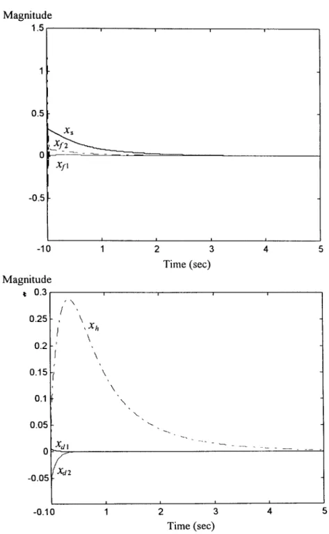
The dynamics of the closed-loop system (75), (79) and (80) under the interconnection shown in Fig. 5 are illustrated in Fig. 7. These figures clearly indicate that the closed- loop system is asymptotically stable at the origin.

VI. Conclusions

In this paper, the stabilization problem of two classes of nonlinear singularly per- turbed systems is discussed. In the first class of systems, the nonlinear functions describing the system dynamics need to be continuously differentiable. While this condition is not necessarily needed in the second class of systems, instead it is assumed that the nonlinear functions describing the system dynamics only satisfy the global Lipschtz condition. The set S(p) of all linear stabilizing compensators given in Theorem 1 plays an important role in our control synthesis, since it can stabilize the reduced- order model of the linearized (or linear) part of the two classes of nonlinear singularly perturbed systems under consideration. We have proved that this can guarantee the stabilization of the first class of systems for a sufficiently small e. However, this is not

972 S . - T . P a n et al. Magnitude 1.5 0.5 -10 -0.5 Magnitude 0.3 , \

/

0.25 ,

/

0.2 0.15 0.1 0.05 xal -0.05

xll

I I I I 1 2 3 4 Time (sec) \ , Xh \ \ \ \ 4 . - - ' 4 I I I I -0.10 1 2 3 4 5 Time (sec)

FIG. 7. The dynamics o f the c l o s e d - l o o p (75), (79) and (80) with e = 0.02 and initial c o n d i t i o n s

Nonlinear Singularly P e r t u r b e d S y s t e m s 973 the case for the other class of systems. The quasi-stability result by Persidskii is then introduced to combine the set S ( p ) obtained from the factorization theory to establish a two-step compensating scheme for stabilizing this class of nonlinear singularly per- turbed systems, provided that e is sufficiently small. The theoretical result demonstrates that, under this two-step compensating scheme, the closed-loop system is asymptotically stable.

R e f e r e n c e s

(1) V. R. Saksena, J. O'Reilly and P. V. Kokotovic, "Singular perturbations and time-scale methods in control theory: survey 1976-1983", Automatica, Vol. 20, pp. 273-293, 1984. (2) P.V. Kokotovic, H. K. Khalil and J. O'Reilly, "Singular Perturbation Methods in Control:

Analysis and Design", Academic Press, New York, 1986.

(3) M. Corless and L. Glielmo, "Robustness of output feedback for a class of singularly perturbed nonlinear systems", in "Proc. 30th IEEE Conf. on Decision and Control", pp. 1066-1071, 1991.

(4) H. K. Khalil, "Feedback control of nonstandard singularly perturbed systems", IEEE

Trans. Automatic" Control, Vol. 34, pp. 1052-1060, 1989.

(5) B. Porter, "Singular perturbation methods in the design of state feedback controllers for multivariable linear systems", Int. J. Control, Vol. 26, pp. 583-587, 1977.

(6) J. O'Reilly, "Dynamical feedback control for a class of singularly perturbed linear systems using a full-order observer", Int. J. Control, Vol. 31, pp. 1-10, 1980.

(7) H. K. Khalil, "On the robustness of output feedback control methods to modeling errors",

IEEE Trans. Automatic Control, Vol. 26, pp. 524-526, 1981.

(8) Z. Gajic and M. T. Lira, "A new filtering method for linear singularly perturbed systems",

IEEE Trans. Automatic Control, Vol. 39, pp. 1952-1955, 1994.

(9) M. Vidyasagar, "Control System Synthesis: A Factorization Approach", MIT Press, Cam- bridge MA, 1985.

(10) S. Lefschetz, "Differential Equations: Geometric Theory", Dover, New York, 1977. (11) B. S. Chen and C. L. Lin, "On the stability bounds of singularly perturbed systems", 1EEE

Trans. Automatic Control, Vol. AC-35, pp. 1265-1270, 1990.

(12) C. L. Lin and B. S. Chen, "On the design of stabilizing controllers for singularly perturbed systems", IEEE Trans. Automatic Control, Vol. 37, pp. 1828-1834, 1992.

(13) S. Sen and K. B. Datta, "Stability bounds of singularly perturbed systems", IEEE Trans.

Automatic Control, Vol. 38, pp. 302-304, 1993.

(14) Z. H. Shao and M. E. Sawan, "Robust stability of singularly perturbed systems", Int. J.