Information Flow between Price Change and
Trading Volume in Gold Futures Contracts
Ramaprasad Bhar*
School of Banking and Finance, University of New South Wales, Australia Shigeyuki Hamori∗∗
Graduate School of Economics, Kobe University, Japan
Abstract
This article examines the pattern of information flow between the percentage price change and the trading volume in gold futures contracts using daily data over a ten-year pe-riod. We employ the robust two-step procedure proposed by Cheung and Ng (1996) to detect the causality in variance. We find evidence of strong contemporaneous causality that is in-dicative of the mixture of distribution hypothesis of information flow. We also detect, al-though not as strong, lagged causality running from percentage price change to trading vol-ume. This indicates mild support for sequential information flow as well directed from price change to trading volume. This is contrary to the documented behavior in agricultural futures and crude oil futures, where bi-directional causality has been reported. We hypothesize that this is probably due to the special nature of gold as a commodity and the fact that the gold market takes on added importance when the equity market underperforms.
Key words: price-volume dynamics; spillover; causality; GARCH model JEL classification: G12; G13
1. Introduction
The volume of contracts traded is an often-quoted statistic for most futures contracts reported by exchanges. The volume data indicates growth or decline of a particular contract. It can also measure shifts in the composition of futures markets as can be illustrated by the enormous growth of financial futures compared to agri-cultural futures. Together with the volume data the price change is also a closely monitored statistic by market participants.
Received June 28, 2004, accepted July 21, 2004.
*We would like to thank an anonymous referee and the editor for many helpful comments and suggestions.
This research was partly supported by a grant-in-aid from the Japan Society for the Promotion of Science. ∗∗Correspondence to: School of Banking and Finance, University of New South Wales, Sydney 2052, Australia. E-mail: R.Bhar@unsw.edu.au.
It is widely believed that arrival of new information induces trading activity in the financial market. Therefore, the trading volume may be thought to carry infor-mation about the aggregate change in expectations about the assets. In addition, any strong relationship between price and trading volume may help devise profitable technical trading rules. Finally, the ability to forecast better price movement in the futures market may improve hedging strategies. Some of the recent studies focusing on these issues are Fujihara and Mougoue (1997), Moosa and Silvapulle (2000), and Kocagil and Shachmurove (1998).
Although most futures contracts have been studied by various researchers, the examination of gold futures contracts and its relationship with price change has not received adequate attention in the published literature. There are some special char-acteristics of this commodity that make it somehow different from other futures con-tracts. Gold can be stored forever and it is not affected by weather conditions. Its ownership change is managed by change in record rather than by physical move-ment. Its supply is not subject to wide swings and in fact the stock of gold is much larger than the annual production. Bertus and Stanhouse (2001) suggest that these characteristics support a better physical/futures pricing relationship for gold com-pared to other futures contracts.
With this background, this paper explores the relationship between price change and trading volume in gold futures contracts using a relatively recent meth-odology based on the cross-correlation function. The aim is to establish evidence of the type of information flow hypothesis the data supports. The gold futures market is also interesting from another perspective. The trading in gold is expected to be in-fluenced by what happens in, say, the equity market. If the equity market underper-forms, then speculative trading in the gold market is likely to rise. At the same time, due to limitations on short sales in the physical market, activities in the futures mar-ket will increase due to relative ease with which short positions can be taken. The combined effect could be different patterns of information flow between percentage price change and trading volume in gold futures as opposed to other commodity futures contracts mentioned before.
2. Brief Literature Survey
The main econometric framework adopted by various researchers is based upon a VAR specification of either the price changes or absolute price changes and trading volume. The Granger causality test then detects the possible direction of the rela-tionship. However, Hiemstra and Jones (1994), Fujihara and Mougoue (1997), and Abhyankar (1998) adopt nonlinear causality tests. These studies claim that the rela-tionship between economic and financial time series is mainly nonlinear.
The published literature suggests two competing hypotheses to explain infor-mation arrival in the market. The mixture of distribution hypothesis suggests that information dissemination is contemporaneous. Some researchers, such as Clark (1973), Karpoff (1987), Tauchen and Pitts (1983), and Andersen (1996), claim that the mixture of distribution hypothesis is consistent with the empirical distribution of
price changes. In this model a positive contemporaneous causality from volume to absolute price changes is implied. Other researchers, such as Copeland (1976) and Jennings et al. (1981), propose sequential arrival of information. In this model, lagged trading volume is expected to imply current absolute price changes and lagged absolute price changes imply current volume.
It is worthwhile to keep in mind some important differences between the physical asset markets and the futures markets that might lead to differences in price volume interaction. In the physical asset market taking short positions is costly whereas in the futures market it is relatively cheap to take short positions. This will eventually lead traders to develop various trading strategies in the futures market which will have complex interaction in the joint distribution of price change and trading volume.
The empirical evidence regarding the price-volume relationship is at best mixed. While many articles provide evidence of bi-directional causality indicating sequen-tial nature of information arrival, some evidence in support of mixture of distribu-tion hypothesis has also been reported. McCarthy and Najand (1993) support the sequential information hypothesis in the currency futures market. Malliaris and Ur-rutia (1998) offer evidence of bi-directional causality in the agricultural futures market. Concerning nonlinear causality, Hiemstra and Jones (1994) find evidence of bi-directional causality in the U.S. stock market, Moosa and Silvapulle (2000) report bi-directional causality in crude oil futures although Fujihara and Mougoue (1997) find only unidirectional causality from volume to price in the case of crude oil.
Also, in several recent empirical studies emphasis has been placed on informa-tion flow between asset markets. Although typically such studies examine causality in mean, there is a growing literature on the interaction between the conditional variances of the assets. This is important since changes in variances reflect the formation arrival in the market and its assimilation by market participants. The in-teraction between the conditional variances indicates the information transmission mechanism between the markets. Gallant et al. (1992), among others, apply a semi-nonparametric method to investigate the price and volume co-movements us-ing daily New York Stock Exchange data. They find four interestus-ing results: (i) a positive correlation between conditional volatility and volume, (ii) that large price movements are followed by high volume, (iii) that conditioning on lagged volume substantially attenuates the “leverage” effect, and (iv) that after conditioning on lagged volume there is a positive risk-return relation. In addition, Ross (1989) uses a no-arbitrage model to explain that the volatility of price changes is the main deter-minant of information transmission. Engle et al. (1990) offer an interpretation that relates the information processing time to variance changes.
It is, therefore, clear that an understanding of the interaction between the condi-tional variances is important to define the information dependency between the two economic variables concerned. Also, the causal pattern in variances provides a use-ful insight into the joint dynamics of the economic variables. Such understanding may lead to better econometric models to characterize these variables.
3. Data and Methodology
Daily data on the gold future price and trading volume from January 3, 1990, to December 27, 2000, are used in this article. The continuous series of futures data are obtained from Datastream and represent NYMEX daily settlement prices. The rate of return is calculated as yt=((P Pt− t-1) /Pt−1) 100× , where Pt is the future price
at time t. Thus the percentage price change is obtained for the period between Janu-ary 4, 1990, and December 27, 2000.
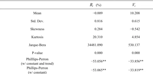
Table 1. Summary Statistics t R (%) Vt Mean −0.009 10.208 Std. Dev. 0.816 0.615 Skewness 0.284 −0.542 Kurtosis 20.310 4.854 Jarque-Bera 34481.090 530.137 P-value 0.000 0.000 Philllips-Perron
(w/ constant and trend) −53.056** −33.856** Phillips-Perron
(w/ constant) −53.065** −33.819** Notes: Rt=((Pt−Pt−1) /Pt−1) 100× and Vt=log(Volume). ** suggests that the null hypothesis of a unit root is rejected at the 1% significance level. P-value is the probability value associated with the Jar-que-Bera test statistic. Phillips-Perron (w/ constant and trend) shows that the auxiliary regression includes a constant and time trend as deterministic terms. Phillips-Perron (w/ constant) shows that the auxiliary regression includes a constant as a deterministic term.
Table 1 shows the summary statistics of the percentage price change and the log of the trading volume. It is clear from the Jarque-Bera test statistic and its corre-sponding p-value that the null hypothesis of a normal distribution is rejected at the 1% significance level for both variables. The existence of a unit root is examined using the Phillips-Perron test (Phillips and Perron, 1988). The empirical results in-dicate that the test statistic is large enough to reject the null hypothesis of including a unit root for both variables.
A two-step procedure proposed by Cheung and Ng (1996) is employed to de-termine mean and variance causal relationships. Their test procedure is based on the residual cross-correlation function (CCF) and is robust to distributional assumptions. In addition, it has a well-defined asymptotic distribution. The great feature of this CCF based method is that it does not depend upon simultaneous modeling of both intra- and inter-variables dynamics. This makes it fairly straightforward to imple-ment in practice. The first stage involves the estimation of appropriate univariate time-series models that allow for time variation in both conditional means and con-ditional variances. In the second stage, the standardized residuals and the squared
standardized residuals are analyzed using the cross-correlation functions to reveal causal pattern in the mean and the variances, respectively. Cheung and Ng (1996) also show that such causal relationships may be utilized to reconstruct the time se-ries models by adding the relevant and significant exogenous variables (i.e., the volume variable for the price change equation and the price change variable for the volume equation). These augmented models may then be estimated and analyzed further to detect the pattern of information flow.
4. Results of the AR-GARCH Model
In this section, we model the dynamics of the percentage price change and trading volume using the AR-GARCH process as follows. The use of the AR struc-ture in the mean equation is justified for the single time series due to its simplicity. The GARCH effect in the variance process is well known for most futures contracts, particularly given the daily frequency. The model is:
1 2 0 p1 , | 1 (0, ) t i i t i t t t t y =a +∑= a y− +ε ε − ∼N σ , (1) 2 3 2 2 2 1 1 1 p p t i i t i i t i σ = +ω ∑=α ε− +∑=β σ − , (2)
where yt is percentage price change or trading volume. Equation (1) shows the
conditional mean dynamics and is specified as a AR(p1) model. Here, ε is the t
heteroskedastic error term with its conditional variance 2
t
σ . Equation (2) shows the conditional variance dynamics and is specified as a GARCH(p2,p3) model. Here,
2
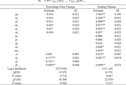
p is the number of ARCH terms and p3 is the number of GARCH terms. The results of fitting AR-GARCH model to the percentage price change and the trading volume are reported in Table 2. Schwarz Bayesian information criteria (SBIC) and diagnostic statistics are used to choose the final models from various possible AR-GARCH specifications. The maximum likelihood estimates confirm that the percentage price change and the trading volume exhibit significant condi-tional heteroskedasticity. The lag order of the AR part in the mean equation (1) is chosen to be 5 for price data and 10 for trading volume data. The GARCH(2,1) model is chosen for the percentage price change, whereas the GARCH(1,1) model is chosen for the trading volume. For price data, the coefficient of the GARCH term is 0.966 and the corresponding standard error is 0.009, indicating substantial persis-tence. For trading volume data, the coefficient of the GARCH term is relatively small, 0.908, and its corresponding standard error is 0.035, indicating less persis-tence compared to the price data. The Ljung-Box statistics (Ljung and Box, 1979)
Q(20) and Q2(20), which are calculated from the first 20 autocorrelation coefficients of the standardized residuals and their squares, indicate that the null hypothesis of no autocorrelation is accepted for both price and trading volume. This suggests that the selected specifications explain the data quite well.
Next, we report causality test results based on the Cheung and Ng (1996) pro-cedure. The test procedure is based on the standardized residuals and their squares estimated from individual AR-GARCH models and is the test for causal
relation-ships in the mean and in the variance. Using the notation in equations (1) and (2), the standardized residual is defined by εt ht . Causality in mean is tested using
cross correlation coefficients between the standardized residuals, whereas causality in variance is investigated using the squares of standardized residuals. It can be shown that, under the no-causality hypothesis, the cross correlations at different lags are independently and normally distributed in large samples. There is no evidence of causality in mean (variance) when all the cross-correlation coefficients calculated from (squares of) standardized residuals, at all possible leads and lags, are not sig-nificantly different from zero. The causality pattern is indicated by significant cross correlation.
Table 2. AR-GARCH Model for Percentage Price Change and Trading Volume
1 2 0 p1 , | 1 (0, ) t i i t i t t t t y =a +∑= a y− +ε ε − ∼N σ 2 3 2 2 2 1 1 1 p p t i i t i i t i σ = +ω ∑=α ε− +∑= β σ−
Percentage Price Change Trading Volume
Estimate SE Estimate SE 0 a −0.016 0.012 3.069** 0.296 1 a −0.033 0.025 0.368** 0.021 2 a −0.013 0.021 0.090** 0.020 3 a −0.045 0.024 0.077** 0.022 4 a 0.017 0.024 0.065** 0.023 5 a 0.034 0.021 0.037 0.022 6 a −0.006 0.021 7 a −0.006 0.020 8 a −0.016 0.020 9 a 0.046* 0.021 10 a 0.043* 0.021 ω 0.001 0.001 0.014* 0.007 1 a 0.177** 0.062 0.041** 0.014 2 a −0.141* 0.060 1 β 0.966** 0.009 0.908** 0.035 Log-Likelihood −2974.926 −2111.105 Q(20) 15.978 16.791 P-value 0.718 0.667 Q2(20) 18.300 22.070 P-value 0.568 0.337
Notes: * indicates significance at the 5% level and ** indicates significance at the 1% level. Boller-slev-Woodridge (1992) robust standard errors are used to calculate the t-value. Q(20) and Q2(20) are the
Ljung-Box statistics with 20 lags for the standardized residuals and their squares.
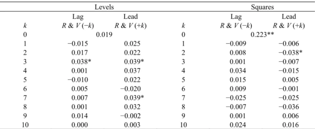
Cross correlations computed from the standardized residuals of the AR-GARCH models of Table 2 are given in Table 3. The “Lag” refers to the number of days that the trading volume data lags behind the percentage price change data. The “Lead” refers to the number of days that the percentage price change data lags behind the trading volume data. Significance of a statistic in the “Lag” column im-plies that the trading volume causes the percentage price change. Similarly, signifi-cance of a statistic in the “Lead” column implies that the percentage price change causes the trading volume. Cross-correlation statistics under “Levels” are based on
standardized residuals themselves and are used to test for causality in mean. Cross-correlation statistics under “Squares” are based on the squares of standardized residuals and are used to test for causality in variance.
Table 3. Cross Correlation Analysis for the Levels and Squares of the Standardized Residuals
Levels Squares
Lag Lead Lag Lead
k R & V (−k) R & V (+k) k R & V (−k) R & V (+k)
0 0.019 0 0.223** 1 −0.015 0.025 1 −0.009 −0.006 2 0.017 0.022 2 0.008 −0.038* 3 0.038* 0.039* 3 0.001 −0.007 4 0.001 0.037 4 0.034 −0.015 5 −0.010 0.022 5 0.015 0.005 6 0.005 −0.020 6 0.009 −0.001 7 0.007 0.039* 7 −0.025 −0.025 8 0.001 0.032 8 −0.007 −0.036 9 0.014 −0.002 9 0.001 0.006 10 0.000 0.003 10 0.024 0.016
Notes: * indicates significance at the 5% level and ** indicates significance at the 1% level.
The empirical results of cross correlations in Table 3 reveal a complex and dy-namic causation pattern between the percentage price change and the trading volume. For instance, the feedback effects in the means involve a high-order lag structure. Trading volume causes the mean percentage price change at lag 3 at the 5% signifi-cance level. The percentage price change causes the mean of the trading volume at lags 3 and 7 at the 5% significance level. Further, there is evidence of strong con-temporaneous causality in variance and mild lagged causality in variance going from the percentage price change to the trading volume but not vice versa. The percentage price change causes the variance of the trading volume at lag 2 at the 5% signifi-cance level. These results show that a proper account of conditional heteroskedastic-ity can have significant implications for the study of price change and trading vol-ume spillovers. The information flows between the price change and trading volvol-ume affect not only their mean movements but also volatility movements in this market. Our main focus here is, however, on the information linkage, as captured by the variance changes, between the trading volume and the percentage price change in gold futures and to examine whether it is different from the documented evidence for other commodity futures contracts. In this context we next move to refining the models in line with the suggestions from Cheung and Ng (1996).
5. Results of the Augmented AR-GARCH Model
Cheung and Ng (1996) illustrate that the cross-correlation statistics offer some useful information on the interaction between time series. Such information can be exploited to build a better model to describe the time-series dynamics of the data. Using the information in Table 3, we estimate an augmented AR-GARCH model for each variable by incorporating the relevant lagged (and squared) data of the other
series to its original AR-GARCH model reported in Table 2.
Based on the previous analysis, we propose the following augmented model for the percentage price change data:
2 5 0 1 3 3 , | 1 (0, ) t i i t i t Rt Rt t Rt R =a +∑= a R− +b V− +ε ε − ∼N σ , (3) 2 2 2 2 1 1 1 Rt i i Rt Rt i σ = +ω ∑=α ε − +β σ − . (4)
Equation (3) shows the mean dynamic for the percentage price change (Rt), where Rt
ε is the heteroskedastic error term with its conditional variance 2
Rt
σ . Equation (3) includes not only the past value of the percentage price change but also the past value of trading volume. The past value of trading volume is included because the empirical results in Table 3 show causality in mean from trading volume to the per-centage price change at lag 3. Equation (4) similarly shows the conditional variance dynamic for the percentage price change and is specified as a GARCH(2,1) model without any augmentation term. There is no additional term in equation (4) because empirical results in Table 3 do not show the causality in variance from trading vol-ume to price change data.
Following the same line of analysis, the augmented model for the trading vol-ume data, on the other hand, is:
2 10 0 1 3 3 7 7 , | 1 (0, ) t i i t i t t Vt Vt t Vt V =a +∑= a V− +b R− +b R− +ε ε − ∼N σ , (5) 2 2 2 2 1 1 1 1 2 2 Vt Vt Vt Rt σ = +ω α ε − +β σ − +γ − . (6)
Equation (5) shows the mean dynamic for the volume (Vt), where ε is the het-Vt
eroskedastic error term with its conditional variance 2
Vt
σ . Equation (5) includes not only the past value of the trading volume but also past values of the percentage price change. The past values of the percentage price change are included because the empirical results in Table 3 show causality in mean from price change to trading volume at lags 3 and 7. Equation (6) shows the conditional variance dynamic for the volume and is specified as a GARCH(1,1) model augmented with the past value of the square of percentage price change. The lagged squared value of price change is included because empirical results in Table 3 show causality in variance from the price change to the trading volume at lag 2.
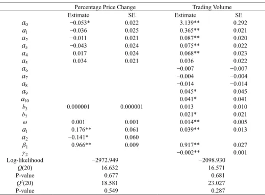
The maximum likelihood estimates are presented in Table 4. Their incremental explanatory power is manifested by changes in the maximum likelihood values. The log likelihood increases from −2974.926 (Table 2) to −2972.949 (Table 4) for the price change model and from −2111.105 (Table 2) to −2098.930 (Table 4) for the trading volume model. The results for the trading volume model indicate that there are significant feedback effects not only in mean but also in variance. The Q(20) and
Q2(20) statistics indicate that the null hypothesis of no autocorrelation is accepted for both price change and trading volume models. This suggests that the selected specifications explain the data well.
Table 4. Augmented AR-GARCH Model for Percentage Price Change and Trading Volume 2 5 0 1 3 3 , | 1 (0, ) t i i t i t Rt Rt t Rt R =a +∑= a R− +b V− +ε ε − ∼N σ 2 2 2 2 1 1 1 1 Rt i i Rt Rt σ = +ω ∑=α ε − +β σ − 2 10 0 1 3 3 7 7 , | 1 (0, ) t i i t i t t Vt Vt t Vt V =a +∑= a V− +b R− +b R− +ε ε − ∼N σ 2 2 2 2 1 1 1 1 2 2 Vt Vt Vt Rt σ = +ω α ε − +β σ − +γ −
Percentage Price Change Trading Volume
Estimate SE Estimate SE 0 a −0.053* 0.022 3.139** 0.292 1 a −0.036 0.025 0.365** 0.021 2 a −0.011 0.021 0.087** 0.020 3 a −0.043 0.024 0.075** 0.022 4 a 0.017 0.024 0.068** 0.023 5 a 0.034 0.021 0.036 0.022 6 a −0.007 −0.007 7 a −0.004 −0.004 8 a −0.014 −0.014 9 a 0.045* 0.045 10 a 0.041* 0.041 3 b 0.000001 0.000001 0.013 0.010 7 b 0.021* 0.021 ω 0.001 0.001 0.014** 0.005 1 a 0.176** 0.061 0.039** 0.013 2 a −0.141* 0.060 1 β 0.966** 0.009 0.917** 0.027 2 γ −0.002** 0.001 Log-likelihood −2972.949 −2098.930 Q(20) 16.632 16.571 P-value 0.677 0.681 Q2(20) 18.581 23.027 P-value 0.549 0.287
Notes: * indicates significance at the 10% level, ** indicates significance at the 5% level, and *** indi-cates significance at the 1% level. Bollerslev-Woodridge (1992) robust standard errors are used to calcu-late the t-value. Q(20) and Q2(20) are the Ljung-Box statistics with 20 lags for the standardized residuals and their squares.
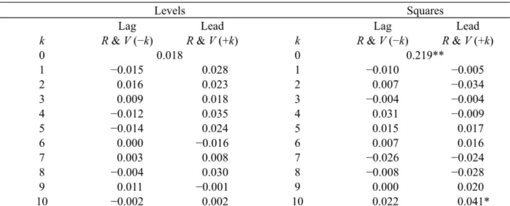
The cross-correlation statistics computed from the standardized residuals of the augmented models are presented in Table 5. Comparing the results in Table 3 and Table 5, it is found that the interaction between the percentage price change and the trading volume in the augmented AR-GARCH models is much weaker than that in the original AR-GARCH models. There is no more residual causality in mean for either equation. However, causality in variance runs from the percentage price change to the trading volume at lag 10 only, in addition to the contemporaneous causality. This is the only statistically significant case. This result suggests that the augmented AR-GARCH model provides a good description of both the percentage price change and the trading volume dynamics and the interaction between the two variables. The finding of strong contemporaneous causality in variance indicates support for the mixture of distribution hypothesis. The variance of the percentage price change has a mild causal effect on the percentage price change variance, which is indicative of the sequential information linkage. This behavior is different from
that cited earlier for agricultural futures and crude oil futures. We hypothesize that this is probably due to the special nature of the gold contracts. Investment in gold becomes attractive when other markets, in particular the equity market, underper-form. As traders take positions in gold futures to reflect their views the information from the price change tends to affect the trading volume.
Table 5. Cross Correlation Analysis for the Levels and Squares of the Standardized Residuals
Levels Squares
Lag Lead Lag Lead
k R & V (−k) R & V (+k) k R & V (−k) R & V (+k)
0 0.018 0 0.219** 1 −0.015 0.028 1 −0.010 −0.005 2 0.016 0.023 2 0.007 −0.034 3 0.009 0.018 3 −0.004 −0.004 4 −0.012 0.035 4 0.031 −0.009 5 −0.014 0.024 5 0.015 0.017 6 0.000 −0.016 6 0.007 0.016 7 0.003 0.008 7 −0.026 −0.024 8 −0.004 0.030 8 −0.008 −0.028 9 0.011 −0.001 9 0.000 0.020 10 −0.002 0.002 10 0.022 0.041* Notes: * indicates significance at the 10% level, ** indicates significance at the 5% level, and *** indi-cates significance at the 1% level.
6. Conclusion
This study examines the joint dynamics of the percentage change in gold fu-tures prices and contract volume using daily data over a ten-year period. The paper presents results from applying the robust two-step technique developed by Cheung and Ng (1996). In the first step we fit appropriate AR-GARCH models to both the price change and the volume series. The cross-correlation functions from the stan-dardized and the squared stanstan-dardized residuals indicate feedback effects between the two series of interest. The econometric model extends the traditional model used to test for causality in mean to also include tests for causality in variance.
Based upon these results we augment the models with relevant lagged variables in the mean and/or the variance equations. These models are then estimated and the marginal improvement in the explanatory power is evidenced from the increase in the likelihood functions. The standardized residuals from these augmented models are then analyzed using cross-correlation functions in order to discover the price change-volume causal pattern. We find evidence of strong contemporaneous causal-ity in variance indicating the mixture of distribution hypothesis of information flow. In addition, the evidence of mild causality in variance running from percentage price change to trading volume with a lag of 10 days indicates some support for the se-quential information flow hypothesis. This behavior of gold futures contracts is dif-ferent from those reported in the literature for agricultural futures and crude oil fu-tures. We hypothesize that this is probably due to the way investment in gold takes place, particularly when the equity market underperforms.
References
Abhyankar, A., (1998), “Linear and Nonlinear Granger Causality: Evidence from the U.K. Stock Index Futures Market,” Journal of Futures Markets, 18, 519-540. Andersen, T. G., (1996), “Return Volatility and Trading Volume: An Information
Flow Interpretation of Stochastic Volatility,” Journal of Finance, 51, 169-204. Bertus, M. and B. Stanhouse, (2001), “Rational Speculative Bubbles in the Gold
Futures Market: An Application of Dynamic Factor Analysis,” Journal of
Fu-tures Markets, 21, 79-108.
Bollerslev, T. and J. M. Wooldridge, (1992), “Quasi-Maximum Likelihood Estima-tion and Inference in Dynamic Models with Time-Varying Covariances,”
Econometric Reviews, 11, 143-172.
Cheung, Y. W. and L. K. Ng, (1996), “A Causality-in-Variance Test and Its Applica-tions to Financial Market Prices,” Journal of Econometrics, 72, 33-48.
Clark, P., (1973), “A Subordinated Stochastic Process Model with Finite Variance for Speculative Process,” Econometrica, 41, 135-155.
Copeland, T. E., (1976), “A Model of Asset Trading under the Assumption of Se-quential Information Arrival,” Journal of Finance, 31, 1149-67.
Engle, R. F., T. Ito, and K. L. Lin, (1990), “Meteor Showers or Heat Waves? Het-eroskedastic Intra-Daily Volatility in the Foreign Exchange Market,”
Econo-metrica, 58, 525-542.
Fujihara, R. A. and M. Mougoue, (1997), “An Examination of Linear and Nonlinear Causal Relationships between Price Variability and Volume in Petroleum Fu-tures Markets,” The Journal of FuFu-tures Markets, 17, 385-416.
Gallant, A. R., P. E. Rossi, and G. Tauchen, (1992), “Stock Prices and Volume,”
Re-view of Financial Studies, 5, 199-242.
Hiemstra, C. and J. D. Jones, (1994), “Testing for Linear and Non-Linear Granger Causality in the Stock Price-Volume Relation,” Journal of Finance, 49, 1639-1664.
Jennings, R. H., L. T. Starks, and J. C. Fellingham, (1981), “An Empirical Model of Asset Trading with Sequential Information Arrival,” Journal of Finance, 36, 143-161.
Karpoff, J. M., (1987), “The Relation between Price Changes and Trading Volume: A Survey,” Journal of Financial and Quantitative Analysis, 22, 109-126. Kocagil, A. E. and Y. Shachmurove, (1998), “Return-Volume Dynamics in Futures
Markets,” The Journal of Futures Markets, 18, 399-426.
Ljung, G. and G. Box, (1979), “On a Measure of Lack of Fit in Time Series Models,”
Biometrika, 66, 265-270.
Malliaris, A. G. and J. L. Urrutia, (1998), “Volume and Price Relationship: Hypothe-sis Testing for Agricultural Futures,” Journal of Futures Markets, 18, 53-72. McCarthy, J. and M. Najand, (1993), “State Space Modeling of Price and Volume
Dependence: Evidence from Currency Futures,” Journal of Futures Markets, 13, 335-344.
Moosa, I. A. and P. Silvapulle, (2000), “The Price-Volume Relationship in the Crude Oil Futures Market: Some Results Based on Linear and Nonlinear Causality
Testing,” International Review of Economics and Finance, 9, 11-30.
Najand, M., H. Rahman, and K. Yung, (1992), “Inter-Currency Transmission of Volatility in Foreign Exchange Futures,” Journal of Futures Markets, 12, 609-620.
Phillips, P. C. B. and P. Perron, (1988), “Testing for a Unit Root in Time Series Analysis,” Biometrika, 75, 335-346.
Ross, S. A., (1989), “Information and Volatility: The No-Arbitrage Martingale Ap-proach to Timing and Resolution Irrelevancy,” Journal of Finance, 44, 1-17. Tauchen, G. and M. Pitts, (1983), “The Price Variability-Volume Relationship on