Local Diagnosability under the PMC Diagnosis Model with Application to Star Graphs

全文

(1)Local Diagnosability under the PMC Diagnosis Model with Application to Star Graphs Guo-Huang Hsua, Jimmy J. M. Tanb Department of Computer Science, National Chiao Tung University, Hsinchu, Taiwan 300, R.O.C. a [email protected], b [email protected] ABSTRACT. In this paper, we introduce a new measure of diagnosability, called local diagnosability, and provide a substructure for determining if a node is locally t-diagnosable under the PMC model. We prove that the local diagnosability of the star graph at each node is equal to its degree. Then, we propose a concept called strong local diagnosability property. We show that an n-dimensional star graph Sn has this strong property, n≥3. Next, we prove that Sn keeps this strong property even if it has up to n-3 faulty edges. Besides, we propose a new diagnosis algorithm for general systems. The time complexity of our algorithm to diagnose all the faulty processors is bounded by O(N logN), where N is the total number of processors.. 1: Introduction In a multiprocessor system, processor fault identification plays an important role for reliable computing. The diagnosability of many interconnection networks have been widely studied [2], [3], [5], [11], [12]. The original diagnostic model was established by Preparata et al. [11]. This model, called PMC diagnosis model, has been extensively studied [6], [7], [8], [11]. In this model, a processor tests a subset of processors, then outputs the testing results. By analyzing the collection of all testing results, all of the faulty processors are identified. The star graph [1] is a popular network topology for multiprocessor systems. An n-dimensional star graph is denoted by Sn, and the diagnosability of Sn is shown to be n-1 under the PMC model, n ≥ 3 [9]. We observe that most previous literatures focused on the diagnosability of a system in a global sense, but ignored some local information. A system is t-diagnosable if all the faulty nodes in the system can be identified provided that the number of faulty nodes does not exceed t. However, it is possible to correctly point out all the faulty nodes in a t-diagnosable system when the number of faulty nodes is greater than t. For example, consider two systems which are m-diagnosable and n-diagnosable, respectively, and m>>n. The diagnosability of a new system which is generated by integrating these two systems with few edges in some way is upper bound by n. However, it is possible to point out all the faulty. nodes even if the number of the faulty ones is between m and n. Hence, if only considering the global faulty/fault-free status, we lose some local details of the system. In this paper, we propose a new measure of diagnosability, called local diagnosability, and study the local diagnosability of each processor instead of the whole system. We show that the diagnosability of a system can be determined by computing the local diagnosability of each node. We also provide a useful substructure to determine the local diagnosability of a processor under the PMC model. Based on the substructure, the local diagnosability of each node in a star graph is shown to be equal to its own degree. Consequently, we propose a concept called strong local diagnosability property. A system is said to have a strong local diagnosability property, if the local diagnosability of each node is equal to its degree. We show that Sn has this strong property. Then, we study the local diagnosability of an incomplete star graph. We show that Sn keeps this strong property even if it has up to (n-3) faulty edges. Finally, we propose a new diagnosis algorithm for general systems. The time complexity of our algorithm to diagnose a given processor is bounded by O(logN) and to diagnose all the faulty processors is bounded by O(N logN), where N is the total number of processors.. 2: Preliminaries and previous results For the graph definition and notation we follow [13]. A multiprocessor system can be modeled as a graph G(V,E), where the set of nodes V represents processors and the set of edges E represents communication links between processors. Let G(V,E) be a graph and v∈V(G) be a node. The degree of v is denoted by degG(v) or simply deg(v). The neighborhood NG(v) of v is the set of all nodes that are adjacent to v in G. Let G1 be a subgraph of G, we shall write the node set of G1 as V(G1). The following is a useful characterization for the distinguishability of two sets of nodes under the PMC model. The symmetric difference of two sets F1 and F2 is defined as the set F1∆F2 = (F1-F2)∪(F2-F1). The PMC model[11] is presented by Preparata, Metze and Chien. In this model, a self-diagnosable. - 159 -.

(2) system is represented by a directed graph T(V,E) in which an edge directed from node u to node v means that u (the tester) can test v (the tested node). The outcome of a test (u,v) is 1(respectively, 0) if u evaluates v as faulty (respectively, fault-free). We assume that the testing results of fault-free nodes are always reliable and the testing results of faulty nodes are unreliable. The set of all testing results is called a syndrome. Formally, a syndrome is any function σ : E → {0, 1}. The set of all faulty processors in the system is called a faulty set. This can be any subset of V(T). For a given syndrome σ, a subset of nodes F⊂V(T) is consistent with σ if the syndrome σ can be produced from the situation that all nodes in F are faulty and all nodes in V-F are fault-free. A syndrome σ is said to be consistent with a faulty set F⊂V(T) if, for a (u,v)∈E(T), such that u∈V-F, σ(u,v) = 1 if and only if v∈F. Since faulty testers can give arbitrary testing results, any syndrome consistent with a faulty set F can occur when faulty processors in the system are exactly those in F. The maximum number of faulty nodes that the system G can guarantee to identify is called the diagnosability of G, written as t(G). Let σF be the set of all syndromes which could be produced if F is the set of faulty nodes. Two distinct sets F1, F2⊂V(G) are said to be distinguishable if σF1∩σF2 = ∅; otherwise, F1, F2 are said to be indistinguishable. We say (F1, F2) is a distinguishable pair if σF1∩σF2 = ∅; otherwise, (F1, F2) is an indistinguishable pair. We need some previous results concerning the t-diagnosable systems. Lemma 1. [4] G(V,E) is t-diagnosable if and only if, for any two distinct sets F1, F2⊂V with |F1| ≤ t and |F2| ≤ t, (F1, F2) is a distinguishable pair. Lemma 2. [4] For any two distinct sets F1, F2⊂V, (F1,F2) is a distinguishable pair if and only if there exists a node u∈V-(F1∪F2) and a node v∈F1∆F2 such that (u, v)∈E. 3: Local diagnosability We observe that the traditional diagnosability discussed in most literatures describes the global status of a system. For this reason, we are motivated to study the local status of each processor instead of the whole system. Given a single node, we require only identifying the status of this particular node correctly. We now propose the following concept. Definition 1. G is locally t-diagnosable at node v if, given a syndrome σF produced by a set of faulty nodes F⊂V containing node v with |F| ≤ t, every set of faulty nodes F’ consistent with σF and |F’| ≤ t, must also contain node v. Definition 2. The local diagnosability of node v, written as tl(v), is defined to be the maximum value of t such that G is locally t-diagnosable at node v.. The following result is another point of view for checking if a node is locally t-diagnosable. Lemma 3. G is locally t-diagnosable at node v if and only if, for any two distinct sets of nodes F1, F2⊂V, |F1| ≤ t, |F2| ≤ t and v∈F1∆F2, (F1, F2) is a distinguishable pair. In the following, we study some properties of a node being locally t-diagnosable, and its relationship between a system being t-diagnosable. Proposition 1. Let G(V,E) be a graph and v∈V be a node with deg(v) = n. The local diagnosability of node v is at most n. Proposition 2. Let G(V,E) be a graph. G is t-diagnosable if and only if G is locally t-diagnosable at every node. By Definition 2 and Proposition 2, we can prove that the diagnosability of a system is equal to the minimum local diagnosability of all nodes of the system. Thus, we have the following theorem. Theorem 1. The diagnosability of G is t if and only if min{tl(v) | for every v∈V} = t. From Theorem 1, we can identify the diagnosability of a system by computing the local diagnosability of each node. Because many well-known systems are node-symmetric, the diagnosability of these system can be easily identified by this effective method. Before studying the local diagnosability of a node, we need some definitions for further discussion. Let S be a set of nodes and v be a node not in S. After deleting the nodes in S from G, we use Cv to denote the connected component which node v belongs to. Now, we propose a necessary and sufficient condition for verifying if a system is locally t-diagnosable at a given node v. Theorem 2. G is locally t-diagnosable at node v if and only if, for each set of nodes S⊂V with |S| = p, 0 ≤ p ≤ t-1 and v∉S, the connected component, which v belongs to in G - S, has at least 2(t - p)+1 nodes. Proof. To prove the necessity, we assume that G is locally t-diagnosable at node v. If the result does not hold, there exists a set of nodes S⊂V with |S| = p, 0 ≤ p ≤ t - 1, v∉S such that the connected component Cv has strictly less than 2(t - p)+1 nodes, |V(Cv)| ≤ 2(t - p). We then arbitrarily partition V(Cv) into two disjoint subsets, V(Cv)=S1∪S2 with |S1| ≤ t - p, |S2| ≤ t - p. Let F1=S1∪S and F2=S2∪S. It is clear that |F1|≤(t-p)+p=t, |F2|≤(t-p)+p=t, the node v∈F1∆F2 and there is no edge between V-(F1∪F2) and F1∆F2. By Lemma 3, (F1, F2) is an indistinguishable pair. This contradicts the assumption that G is locally t-diagnosable at node v. We now prove the sufficiency by contradiction. Suppose G is not locally t-diagnosable at node v, then, there exists an indistinguishable pair (F1, F2) with |F1|≤t,. - 160 -.

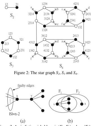
(3) |F2|≤t and v∈F1∆F2. By Lemma 2, there is no edge between V-(F1∪F2) and F1∆F2. Let S=F1∩F2 with |S|=p, 0 ≤ p ≤ t - 1 and v∉S. F1∆F2 is disconnected from other parts after removing all the nodes in S from G. We observe that |F1∆F2| ≤ 2(t - p). Thus, the connected component Cv has at most 2(t - p) nodes and |V(Cv)| ≤ 2(t - p). This contradicts the assumption that the connected component Cv has to satisfy |V(Cv)| ≤ 2(t - p) + 1. Hence, the theorem holds. We now propose a special substructure. This provides us with an efficient and simple method to identify the local diagnosability of each node of a system under the PMC diagnosis model. Definition 3. Let G(V,E) be a graph, v∈V be a node and k be an integer, k ≥ 1, a substructure H(v, k) of order k at node v is defined to be the following graph, H(v, k) = [V(v; k), E(v; k)] which is composed of 2k+1 nodes and of 2k edges as illustrated in Figure 1, where V(v; k) = {v}∪{xi, yi | 1 ≤ i ≤ k}, E(v; k) = {(v, xi), (xi, yi) |1 ≤ i ≤ k}.. 4: Strong Local Diagnosability Property We use the star graph as an example to introduce our concept of the strong local diagnosability property. An n-dimensional star graph Sn is an undirected graph consisting of n! nodes and (n-1)n!/2 edges. The set of nodes V(Sn)={u1u2…un | ui∈<n> and ui ≠ uj for i ≠ j}, where <n> is the set {1, 2, …, n}. The adjacent is defined as follows: u1u2…ui…un is adjacency to v1v2…vi…vn through an edge of dimension i with 2 ≤ i ≤ n if vj = uj for j∉{1, i} vi = ui and vi = u1. For example, in S4 containing 4! nodes, two nodes 1234 and 4231 are neighbors and joined through an edge labeled 4. In Sn, each node is connected to n-1 neighbors by n-1 edges. Each Sn can be decomposed into n subgraph Sn-1. The star graph S2, S3 and S4 are shown in Figure 2. Now we propose the following two concepts.. Figure 1: A substructure H(v; k) of order k at node v. Following Theorem 2 and Definition 3, we propose a sufficient condition for verifying if it is locally t-diagnosable at a given processor in a system.. Figure 2: The star graph S2, S3 and S4.. Theorem 3. G is locally t-diagnosable at node v if G contains a substructure H(v; t) of order t at node v Proof. We use Theorem 2 to prove this result. Assume that G contains a substructure H(v; t) at node v. Let ei=(xi, yi) be the edge for each i, 1 ≤ i ≤ t, with respect to H(v; t). The number of nodes of the connected component including node v is at least 2t + 1. Let S⊂V(G) be a set of nodes with |S| = p, 0 ≤ p ≤ t - 1 and v∉S. After deleting S from V(G), there are at least (t - p) complete ei's still remain in T1(v;t). Therefore, the number of nodes of the connected component Cv is at least 2(t-p)+1. By Theorem 2, G is locally t-diagnosable at node v. The proof is complete. By Theorem 3, we have the following result. Theorem 4. Let G(V,E) be a graph and v∈V be a node with deg(v) = n. The local diagnosability of node v is n if G contains a substructure H(v; n) of order n at node v.. Figure 3: An indistinguishable pair (F1, F2), where |F1| = |F2| = n - 1. Definition 4. A node v has the strong local diagnosability property if the local diagnosability of node v is equal to its degree. Definition 5. A graph has the strong local diagnosability property if, every node in the graph has the strong local diagnosability property. Following Definition 4 and 5, and by using a simple induction, we can prove the following theorem. Due to the page limit, we omit this routine proof. Theorem 5. Sn has the strong local diagnosability property, n ≥ 3.. - 161 -.

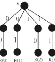
(4) We now consider a system which is not node-symmetric. Let G(V,E) be a graph and S⊂E(G) be a set of edges. Removing the edges in S from G, the degree of each node in the resulting graph G - S is called the remaining degree of v, and is denoted by degG-S(v). We consider a faulty star graph Sn with a faulty set S⊂E(Sn), n ≥ 3. We shall prove that Sn has the strong local diagnosability property even if it has up to (n - 3) faulty edges. The number (n - 3) is optimal in the sense that a faulty Sn cannot be guaranteed to have this strong property if there are (n-2) faulty edges. As shown in Figure 3, we take a node v∈V(Sn) and a node x which is an adjacent neighbor of v. Let S = {(y, x)∈E(Sn) | node y is directly adjacent to x} – {(v, x)}, then |S| = n–2 and the remaining degree of v in Sn-S is n-1. Let F1 = (NSn-S(v) - {x})∪{v} and F2 = NSn-S(v), then |F1| = |F2| = n - 1 and v∈F1∆F2. It is clear that there is no edge between V-(F1∪F2) and F1∆F2. By Lemma 2, (F1, F2) is an indistinguishable pair, hence tl(v) ≠ degSn-S(v) = n-1. Therefore, Sn-S may not have this strong property, if |S| ≥ n - 2. Again, we can use induction method to prove the following theorem. Theorem 6. Let Sn be an n-dimensional star graph with n ≥ 3, and S⊂E(Sn) be a set of edges, 0 ≤ |S| ≤ n - 3. Removing all the edges in S from Sn, the local diagnosability of each node is still equal to its remaining degree. We have the following corollary.. Figure 4: four different output states. Suppose that there is a substructure H(v; n) of order n at node v, where v has degree n. By Theorem 4, the local diagnosability of v is limited to n. Therefore, we may not be able to identify all the faulty nodes, if the number of faulty nodes in H(v; n) is n+1 or more. Hence, we assume that the number of faulty nodes is at most n. Under this assumption, we propose the following algorithm to determine whether node v is faulty or not. Theorem 7. Let v be a node with degree n in G(V,E). Suppose that there is a substructure H(v; n) of order n at node v and the number of faulty nodes is at most n. The following two conditions are satisfied: 1. the node v is fault-free if |R(0)| ≥ |R(2)|, and 2. the node v is faulty if |R(0)| < |R(2)|. Proof. Let li = (xi, yi) be an ordered double, 1 ≤ i ≤ n, with respect to H(v; n). First, we prove the condition 1 by contradiction. Assume that v is faulty, then the counting of all the other faulty nodes is as follows: For those li with result r(0), there are at least 2 faulty nodes which are xi, yi.. Corollary 1. Let Sn be an n-dimensional star graph with n ≥ 3, and S⊂E(Sn) be a set of edges, 0 ≤ |S| ≤ n - 3. Then, Sn - S has the strong local diagnosability property.. For those li with result r(1), there is at least 1 faulty node which is xi. For those li with result r(2), the number of faulty nodes is uncertain.. 5: A Diagnosis Algorithm We now introduce a diagnosis algorithm to determine if a node is faulty or not for a given syndrome under the PMC model. Given a substructure H(v; n) of order n at node v, there are communication links between v and xi, xi and yi, for all 1 ≤ i ≤ n, xi and yi can be the tester of the PMC model. After the test, each tester has a testing result denoted by 0 (1, respectively) representing the approval (disapproval, respectively). We define ri = (r1, r2), where r1 is the result of xi testing v and r2 is the result of yi testing xi. Then, ri can be in one of the four different states which are r(0) = (0, 0), r(1) = (0, 1), r(2) = (1, 0) and r(3) = (1, 1) (as illustrated in Figure 4). Let R(k) be the collection of all r(k), for all 0 ≤ k ≤ 3. Obviously, 3 | R(k ) |= n .. For those li with result r(3), there is at least 1 faulty node which is either xi or yi. Thus, the number of faulty nodes is at least 1 + 2|R(0)| + 3. |R(1)| + |R(3)| =. |R(k)| + (1 + |R(0)| - |R(2)|). By the k =0. assumption that |R(0)| ≥ |R(2)|, the number of faulty nodes is strictly more than n. This contradicts to the assumption that the number of faulty nodes is at most n. Therefore, the node v is fault-free. Next, we prove the condition 2 by contradiction again. Assume that v is fault-free, then the counting of all the other faulty nodes is as follows:. k =0. For those li with result r(0), the number of faulty nodes is uncertain. For those li with result r(1), there is at least 1 faulty node which is either xi or yi. For those li with result r(2), there are at least 2 faulty nodes which are xi and yi.. - 162 -.

(5) For those li with result r(3), there is at least 1 faulty node which is xi. Thus, the number of faulty nodes is at least |R(1)| + 3. |R(k)| + (|R(2)| - |R(0)|). By the. 2|R(2)| + |R(3)| = k =0. assumption that |R(0)| < |R(2)|, the number of faulty nodes is larger than n. This contradicts to the assumption that the number of faulty nodes is at most n. Therefore, the node v is faulty. This completes the proof.. In [10], Lai et al. introduced a measure of diagnosability called conditional diagnosability by restricting that a faulty set cannot contain all the neighbors of any node. Therefore, it is also an attractive work to develop more different measures of local diagnosability based on network reliability.. 6: References [1] S. B. Akers, “A group-theoretic model for symmetric interconnection network,” IEEE Trans. Computers, vol. 38, no. 4, pp. 555-566, 1989.. We now measure the time complexity of our algorithm to diagnose all the faulty nodes in a system. For many well-know general systems with N nodes, the degree of each node is in the order of logN. For example, the n-dimensional Hypercube Qn has N = 2n nodes and the degree of each node is n, n = logN; the n-dimensional star graph Sn has N = n! nodes and the degree of each node is n-1 = O(n) = O(logN/log n) = O(logN/log logN). We assume that a testing result of each tester is directly stored in a syndrome table. Given a substructure H(v; n) of order n at node v, assume the time for looking up the testing result of a tester in the syndrome table is constant c. Then, the time needed for determining the faulty or fault-free status of a node v is 2clogN = O(logN). Consequently, the total time to diagnose all the faulty nodes is bounded by O(N logN).. [4] A. T. Dahbura and G. M. Masson, “An O(n2.5) Faulty Identification Algorithm for Diagnosable Systems,” IEEE Trans. Computers, vol. 33, no. 6, pp. 486-492, June 1984.. 6: Conclusions. [5] A. D. Friedman and L. Simoncini, “System-Level Fault Diagnosis,” The Computer J., vol. 13, no. 3, pp. 47-53, Mar. 1980.. In this paper, we propose a new concept of local diagnosability for a system and derive a substructure for determining if a system is locally t-diagnosable at a given node. Through this concept, the diagnosability of a system can be determined by computing the local diagnosability of each node. We also introduce a concept for system diagnosis, called strong local diagnosability property. We prove that the star graph has this strong property. Then, we consider an n-dimensional faulty star graph Sn with a set of faulty edges S⊂E(Sn), 0 ≤ |S| ≤ n-3, n ≥ 3. We prove that a faulty star graph Sn-S keeps this strong property. According to Theorem 1, the global diagnosability of Sn-S is equal to the minimum local diagnosability of all nodes. Finally, we propose a new diagnosis algorithm for general systems. The time complexity of our algorithm to diagnose all the faulty processors is bounded by O(N logN), where N is the total number of processors. We use the star graph as an example to introduce the concepts of the local diagnosability, the local structure and the strong local diagnosability property. In fact, many well-known systems also have the local structure and this strong property. There are several different fault diagnosis models in the area of diagnosability. It is worth investigating, under various models, whether a system has this strong local diagnosability property after removing some edges.. [2] A. Bagchi, “A Distributed Algorithm for System-Level Diagnosis in Hypercubes,” Proc. IEEE Workshop Fault-Tolerant Parallel and Distributed Systems, pp. 106-133, July 1992. [3] A. Bagchi and S. L. Haiimi, “An Optimal Algorithm for Distributed System Level Diagnosis,” Proc. IEEE CS 21st Int'l Symp. Fault-Tolerant Computing, pp. 214-221, 1991.. [6] S. L. Hakimi and A. T. Amin, “Characterization of connection assignment of diagnosable systems,” IEEE Trans. on Computers, vol. 23, no. 1, pp. 86-88, Jan. 1974. [7] S. H. Hosseini, J. G. Kuhl and S. M. Reddy, “A Diagnosis Algorithm for Distributed Computing Systems with Dynamic Failure and Repair,” IEEE Trans. on Computers, vol. 33, no. 3, pp. 223-233, Mar. 1984. [8] S. Huang, J. Xu and T. Chen, “Characterization and Design of Sequentially t-Diagnosable Systems," Proc. IEEE CS 19th Int'l Symp. Fault Tolerant Computing, pp. 554-559, 1989. [9] A. Kavianpour, “Sequential diagnosability of star graphs,” J. Comput. Electrical Engrg., vol. 22, no. 1, pp. 37-44, 1996. [10] P. L. Lai, Jimmy J. M. Tan, C. P. Chang, and L. H. Hsu, “Conditional Diagnosability Measures for Large Multiprocessor Systems,” IEEE Trans. on Computers, vol. 54, no. 2, pp. 165-175, Feb. 2005. [11] F. P. Preparata, G. Metze and R. T. Chien, “On the Connection Assignment Problem of Diagnosis. - 163 -.

(6) Systems,” IEEE Trans. on Electronic Computers, vol. 16, no. 12, pp. 848-854, Dec. 1967. [12] A. K. Somani, V. K. Agarwal and D. Avis, “A Generalized Theory for System Level Diagnosis,” IEEE Trans. on Computers, vol. 36, no. 5, pp. 538-546, May 1987. [13] D. B.West, Introduction to Graph Theory. Prentice Hall, 2001.. - 164 -.

(7)