基於多特徵探勘的電腦遊戲個人化推薦

全文

(1) . 國立高雄大學資訊工程學系研究所碩士論文. 基於多特徵探勘的電腦遊戲個人化推薦 Personalized Recommendation of PC Games Based on Multiple Features Mining. 研究生：許聰榮撰指導教授：洪宗貝博士共同指導：藍國誠博士. 中華民國 101 年 7 月 .

(2) . 致謝首先，誠摯感謝指導教授洪宗貝教授與共同指導教授藍國誠教授。兩位教授在研究過程中給予詳細與全面性的指導，並提供許多寶貴的研究經驗、資源，讓我在研究上得以順利進行。特別感謝藍國誠教授對本論文付出之心力，從訂定研究方向、研究主題、方法與架構，到最後的論文撰寫始終在旁協助，在百忙之中撥空與學生討論及解決問題，對本論文細心審閱及不吝指教，讓整個研究工作能夠順利的進行並有所成果。同時，我要感謝我的碩士論文口試委員，林威成教授、李詠騏教授以及黃健峯教授。感謝您們撥空來參加我的碩士論文口試，並且對於我的碩士論文內容給予寶貴的建議及指導，使本論文更加完善。其次，感謝邱菊添學長在研究過程中，總是能適時地給予協助、解惑與經驗的傳承，讓我能夠在研究上能順利及快速的入門。另外，也非常感謝實驗室的學長們、同學與學弟妹們，以及曾經幫助過我的人，平時給予協助與鼓勵，也因為有你們共同努力及教學相長，使我的困惑之處因此可以獲得解答。最後，由衷感謝我的父母親與家人，給予支持，特別是我的女友玲媚，在求學這二年來，感謝有妳的陪伴、督促及照顧，才能讓我在這研究過程當中，快速的學習及成長。在此，謹以本論文表達心中對您們最誠摯的感謝。. i .

(3) . 基於多特徵探勘的電腦遊戲個人化推薦指導教授：洪宗貝博士國立高雄大學資訊工程學系共同指導：藍國誠博士國立成功大學資訊工程學系學生：許聰榮國立高雄大學資訊工程學系. 中文摘要. 近年來，隨著網際網路的發達以及遊戲開發技術的成熟，造就電腦遊戲市場的快速成長，玩家在面對琳琅滿目的電腦遊戲當中，不容易選擇適合玩家所喜好的遊戲。正因為如此，如何幫助玩家選擇適合、感興趣、相關性高的遊戲來推薦給玩家，成為一個重要的研究議題。在本篇論文中，我們提出一個有效的推薦策略，採用基於 Apriori 加權的資料探勘方法，從玩家的遊戲歷史記錄，找出不同群體玩家共通的遊戲特徵項目，作為多特徵推薦系統的基礎，並應用 CAST 分群的方法，找出玩家之間的相似度，再應用 PageRank 演算法，推算出玩家之間共同喜好的遊戲排名清單，並依據個體玩家的喜好，匹配相似的群體玩家，採用群體玩家的喜好遊戲排名清單，來協助玩家更容易找到感興趣的遊戲。本研究中所提出之推薦策略，應用於實作之遊戲推薦系統，並依實驗結果的資料分析，衡量出基於多特徵探勘的推薦結果。實驗結果顯示，所提出策略的有效性。. 關鍵字：推薦系統、資料探勘、多特徵、協同過濾、CAST、PageRank。. ii .

(4) . Personalized Recommendation of PC Games Based on Multiple Features Mining Advisor: Dr. Tzung-Pei Hong Department of Computer Science and Information Engineering National University of Kaohsiung Co-advisor: Dr. Guo-Cheng Lan Department of Computer Science and Information Engineering National Cheng Kung University Student: Tsung-Jung Hsu Department of Computer Science and Information Engineering National University of Kaohsiung. ABSTRACT With rapid in Internet and game-playing technologies, the computer games market has seen explosive growth in recent years. However, it is often not easy for a player to find a game that meets their preferences. In this paper, we propose a recommendation strategy based on a player’s game-playing history, and use the Apriori-based weighted data mining method to identify common features of games among different groups of players. The recommendation system considers multiple features and adopts the CAST clustering method to assess the similarities among players. It then modifies the PageRank algorithm to calculate the different groups of players in the game ranked list. The system then matches the game ranked list of the groups of similar players, and thus helps players to find games which they are more likely to be interested in. The recommendation strategy proposed in this thesis is also used for a real implementation of a game recommendation system, and experiments are carried out. The results show the effectiveness of the proposed strategy.. Keywords: Recommendation System, Data Mining, Multiple Feature, Collaborative Filtering, CAST, PageRank. iii .

(5) . Contents 致謝 ............................................................................................................. i 中文摘要 .................................................................................................... ii ABSTRACT ............................................................................................. iii Contents .................................................................................................... iv List of Figures .......................................................................................... vi List of Tables ........................................................................................... vii Chapter 1. Introduction ......................................................................... 1. Chapter 2. Review of Related Works ................................................... 3. 2.1. Recommendation System .......................................................................... 3. 2.2. Association-Rule Mining........................................................................... 4. 2.3. Weighted Sequential Pattern Mining ......................................................... 6. 2.4. Clustering Techniques ............................................................................... 8. 2.5. PageRank Algorithm ................................................................................. 8. Chapter 3. Problem Definition and Statement .................................. 10. Chapter 4. The Research Framework ................................................ 20. 4.1. Proposed recommendation framework .................................................... 22. 4.2. Phase 1: Data Pre-processing .................................................................. 27. 4.3. Phase 2: Multi-feature Mining................................................................. 28. 4.4. Phase 3: Player Clustering ....................................................................... 30. 4.5. Phase 4: Games Ranking ......................................................................... 31. 4.6. Games Recommendation ......................................................................... 33. Chapter 5 5.1. Experimental Evaluation.................................................. 36 Experimental Dataset............................................................................... 36 iv . .

(6) . 5.2. Chapter 6. Evaluation on a Real Dataset ................................................................... 37. Conclusions and Future Works ....................................... 43. References ............................................................................................... 45. v .

(7) . List of Figures Figure 1: The proposed recommendation system framework. .............................. 21 Figure 2: The link relationship of game items for this example. ........................... 32 Figure 3: The process of calculating the average PR value of each cluster. ......... 35 Figure 4: The classification of the game items. ....................................................... 37 Figure 5: Comparison the results with different min_supp thresholds................. 40 Figure 6: Comparison of the results with different similarity thresholds. ........... 40 Figure 7: The different clustering counts compare the recommended degree results. ..................................................................................................................................... 41 vi .

(8) . List of Tables Table 1: Some records from the original log ........................................................... 10 Table 2: The converted transaction database TDB in this example. ..................... 12 Table 3: The converted sequence database SDB in this example. ......................... 15 Table 4: The feature table for the five players in this example. ............................ 17 Table 5: The adjacency matrix for this example. .................................................... 32 Table 6: The reverse adjacency matrix for this example. ...................................... 32 Table 7: The page rank values of all game items for this example. ....................... 33 Table 8: Statistical data collected from the players’ historical records. ............... 37 Table 9: Weights of the different time Periods. ....................................................... 38 Table 10: Numbers of features and consume time along with different thresholds. ..................................................................................................................................... 38 . vii .

(9) . Chapter 1 Introduction Currently, recommendation systems from the field of artificial intelligence are being applied to a wide range of practical applications, such as music, image, and tour recommendation systems. Such recommendation models can be trained and built based on information of the users’ various preferences, and this data is then used to provide personalized recommendation for each user. Online are increasingly popular, and thus there are now a vast number of games for users to choose from. However, it is generally difficult and time-consuming for user to find a game that they are interested in, and thus there is a need for a recommendation system to help them make their decisions. Herlocker [3] et al. used player data to develop a highly automated recommendation system, which applied the views of user groups to identify items of interest to individual players according to a variety of criteria. However, the features of the players were directly acquired from the players’ current data in order to build the recommendation system, and it might be more suitable if these were drawn from the players’ historical data by using various mining techniques. It is thus necessary to develop an intelligent recommendation model that considered multiple features in an online game website environment. Chen et al. proposed a multi-criteria 1 .

(10) . game recommendation approach, based on the players’ experience [2]. In the thesis, we propose a novel intelligent system for recommending the top-k games items for players in an online game website. To consider recent popular games, the recommendation mechanism also considers the weights of different time periods, and then explores multi-feature information from the players’ historical data by using weighted itemset mining and weighted sequential pattern mining techniques. Based on the mined features, a traditional clustering algorithm, named CAST, is used to group players into several groups with high similarity values. Next, the concept of the PageRank algorithm is utilized to generate a of ranked game items for each player group. Finally, the recommendation model gives the top-k game items for one player according to the ranked list of that player’s corresponding group with highest similarity when the player logs into the online game website. The remainder of this thesis is organized as follows. Some related works are reviewed in Section 2. The problem to be solved and its definitions are stated in Section 3. The execution process of the proposed algorithm is described in Section 4. Finally , the conclusions and suggestions for future works are given in Section 5.. 2 .

(11) . Chapter 2 Review of Related Works In this section, some related studies on recommendation systems, weighted association-rule mining, and weighted sequential pattern mining are briefly reviewed.. 2.1. Recommendation System. The concept of a recommendation system, which considers the features of users to evaluate a large number of possible choices for items, was first proposed in 1997 [8]. With the help of the recommendation mechanism, the most interesting or useful information could be selected and provided the users. The existing recommendation systems can be divided into three types, content-based, collaborative filtering, and hybrid recommendation systems. Two approaches are used in content-based recommendation mechanisms, information filtering [5] and information retrieval [7]. The features required by both approaches are found from the textual information of related to items and users’ historical data, and then user preference data can be derived and obtained from these features. In general, the users’ historical data can be collected from the users’ explicit feedback behaviors, or from the implicit feedback behaviors of rating scores for the items. 3 .

(12) . For collaborative filtering mechanisms, the main assumption is that the user should give the same or similar scores to similar. Further, collaborative filtering mechanisms can be also divided into two kinds, memory-based and model-based. Since memory-based collaborative filtering approaches do not filter any of the scores recorded for each user, and thus all the records are used to calculate the prediction scores of items. Such approaches thus need considerable computational time to build their recommendation models. Model-based collaborative filtering approaches are slightly different, and are based on the assumption that similar users in a community may be interested in the same items. Although content-based and collaborative filtering recommendation systems can both obtain significant results, there are some problems with the two approaches. For example, content-based recommendation systems can not recommend items for new users, since there is historical data for them. In addition, collaborative filtering recommendation systems do not work when there is insufficient data. Accordingly, a hybrid approach can be used that combines the advantages of both methods.. 2.2. Association-Rule Mining. In the field of knowledge discovery, the main purpose of data mining is to extract useful patterns or rules from a set of data. One common type of data mining is to derive 4 .

(13) . association rules from transaction data, such that the presence of certain items in a transaction will imply the presence of some other items. In order to achieve this, Agrawal et al. proposed several mining algorithms based on the concept of large itemsets to find association rules from transaction data [6]. The Apriori algorithm for association-rule mining was the most well-known of these. The process of association-rule mining can be divided into two main phases. In the first phase, candidate itemsets are generated and counted by scanning transaction data. If the count of an itemset in the transactions is larger than or equal to a pre-defined threshold value (called the minimum support threshold), the itemset is identified as a frequent one. Itemsets containing only one item are processed first. Frequent itemsets containing only single items are then combined to form candidate itemsets with two items. The above process is then repeated until no candidate itemsets are generated. In the second phase, association rules are derived from the set of frequent itemsets found in the first phase. All possible association combinations for each frequent itemset are formed, and those with calculated confidence values larger than or equal to a predefined threshold (called the minimum confidence threshold) are output as association rules. However, an itemset in association-rule mining only considers the frequency of the itemset in the databases, and the same significance is assumed for all items in the itemset. In reality, however, the importance of items in a database may be different according to different factors, such as profit and cost. For example, LCD TVs may not 5 .

(14) . have high frequency, but are a high-profit product when compared to food or drink in a database. Therefore, some useful information may not be discovered by using traditional frequent itemset mining techniques. To handle this problem, Yun et al. proposed an approach called weighted itemset mining [11], used to find weighted frequent itemsets in transaction databases. The weights of the items in a database used for weighted itemset mining can be flexibly given by users, and the average-weight function in Yun et al. [11] was designed to evaluate the weight of an itemset in a transaction. Different from frequent itemsets that only consider the frequency, the itemsets that are found with high-weight values can be used to aid managerial decision-making.. 2.3. Weighted Sequential Pattern Mining. In general, the transaction time (or time stamp) of each transaction for real-world applications is usually recorded in a database. The transaction can then be listed as a time-series data (called sequence data) in the order that the transactions occurred. Sequential pattern mining was developed to handle such data,. and the three algorithms,. AprioriAll, AprioriSome, DynamicSome, were also proposed to find the sequential patterns in sequence data. A similar problem to that mentioned previously for items with the same 6 .

(15) . significance in weighted itemset mining exists for sequential pattern mining. To deal with this, Yun et al. thus proposed weighted sequential pattern mining [11], to find weighted sequential patterns from sequence data. In this, different weights are given to items based on various factors, such as their profits, costs, user preferences, and then the actual importance of a pattern can be more easily recognized than is possible with traditional sequential pattern mining. Different from the functions in weighted itemset mining, the time factor is used to develop a new average-weight function [11], and this can then be applied to identify the weight value of a pattern in a sequence. However, based on the function, the downward-closure property in traditional sequential pattern mining cannot be maintained with weighted sequential pattern mining. To address the problem, a new upper-bound mode, in which the maximum weight in sequence data is regarded as the upper-bound of each sequence, was directly derived from Yun et al.’s proposed model for weighted itemset mining [11]. However, a huge amount of unpromising subsequences still need to be generated by using the traditional upper-bound model [11] for mining, and thus its performance is not very good. This is one of the reasons that motivates our goal to more effectively and efficiently mining weighted sequential patterns from a set of sequences.. 7 .

(16) . 2.4. Clustering Techniques. In the field of data mining, clustering techniques is used to cluster a set of objects into a set of groups with highly similar values, based on information about their features. The techniques used to achieve this are also called unsupervised data mining. In the thesis, hierarchical-based clustering techniques are used to group players into several groups. This is because hierarchical clustering approaches can produce cluster agglomerative or divisive results by using a tree structure. The CAST algorithm, a hierarchical-based technique, was proposed by Ben-Dor et al. in 1999 [1], and it remains the most efficient of existing clustering methods. The main concept of the algorithm is that items are repeatedly linked together and then put into the hierarchical tree structure by based on the average similarity among them. When all the items in a set are put into the hierarchical tree structure, the minimum similarity threshold is then used to divide the tree into several groups. That is, the similarity of the items in the groups has to satisfy a minimum similarity threshold. The detailed process of the CAST algorithm is given in Ben-Dor et al. [1].. 2.5. PageRank Algorithm. The PageRank algorithm [4], which is a link-based analysis technique, was first proposed in 1998. The main concept of PageRank is that each page has an equivalence 8 .

(17) . vote based on its links with other pages. That is, the vote of one page is shared by its out-links to other pages, and the focal page itself can obtain votes based on its in-links relationship to other pages. Based on the in-links and out-links, we can thus know the significance of each page, and then rank the pages in descending order of this. The concept of the PageRank algorithm is applied to the game items in our study, and used to rank the game items in a player group.. 9 .

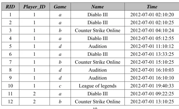
(18) . Chapter 3 Problem Definition and Statement To clearly explain the problem of building a recommendation model, assume there are five players in the original log file on the online game website, and some of the five players’ historic records is shown in Table 1 ordered by time, in which there are six attribute fields, RID (Record ID), Player_ID, Game, Category, Name, and Time. Also, assume that there are four game items in the online game list, called Diablo III, CS Online, Audition, and League of Legends. To simplify the game names, four letters, a, b, c, and d, are used hereafter. With regard to the problem discussed in this work, a set of terms related to a recommendation model is first defined, as follows.. Table 1: Some records from the original log RID. Player_ID. Game. Name. Time. 1. 1. a. Diablo III. 2012-07-01 02:10:20. 2. 1. a. Diablo III. 2012-07-01 02:10:25. 3. 1. b. Counter Strike Online. 2012-07-01 04:10:24. 4. 1. a. Diablo III. 2012-07-01 05:12:55. 5. 1. d. Audition. 2012-07-01 11:10:12. 6. 1. a. Diablo III. 2012-07-01 13:33:25. 7. 1. b. Counter Strike Online. 2012-07-01 15:10:25. 8. 1. d. Audition. 2012-07-01 16:10:03. 9. 1. d. Audition. 2012-07-01 16:10:10. 10. 1. c. League of legends. 2012-07-01 19:40:33. 11. 2. a. Diablo III. 2012-07-01 09:22:25. 12. 2. b. Counter Strike Online. 2012-07-01 13:10:25. 10 .

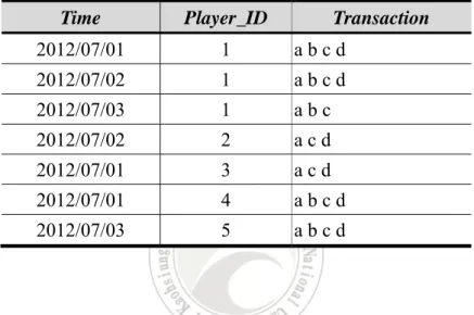
(19) . 13. 2. d. Audition. 2012-07-01 16:10:03. 14. 2. d. Audition. 2012-07-01 16:10:10. 15. 2. c. League of legends. 2012-07-01 19:20:29. Definition 1. Dplayers = {r1, r2, ..., rm} is a set of player records, where rm represents the m-th player record, and there are the values of six attribute fields, namely RID, Player_ID, Game, Category, Name, and Time. For example, in Table 1, r3 is the third record, and the corresponding values of the six fields for the record r3 are 3, 1, b, 1, “CS Online”, and “2012-07-01 04:10:24”, respectively. Definition 2. An itemset X is a subset of items, X  I. If |X| = k, the itemset X is called a k-itemset. I = {i1, i2, ..., in} is a set of game items. In this study, there are only four game items, and, as noted above, the four letters, a, b, c, and d, are used to replace these. For example, in Table 1, the item b in r3 stands for “CS Online”. To find frequent itemsets and sequential patterns from the set of player records Dplayers, the set of player records Dplayers has to be converted into the data formats required by both mining techniques. The terms related to the process of data transformation are described below. Definition 3. TDB = {Trans1, Trans2, ..., Transl} is a set of player transactions with game items in one day, where Transl in Dplayers represents the l-th transaction and consists of the unique game items in all one player’s records in time order in one day. For example, in Table 1, since the first transaction for player p1 includes the ten records 11 .

(20) . that are from the first to the tenth records, the first transaction Trans1 for the player p1 is {abcd}. In this study, assume all the player records in Table 1 have been converted into the transaction database according to the third definition, as shown in Table 2.. Table 2: The converted transaction database TDB in this example. Time. Player_ID. Transaction. 2012/07/01. 1. abcd. 2012/07/02. 1. abcd. 2012/07/03. 1. abc. 2012/07/02. 2. acd. 2012/07/01. 3. acd. 2012/07/01. 4. abcd. 2012/07/03. 5. abcd. Definition 4. T = {t1, t2, ..., tj} is a set of mutually disjoint time periods, where tj denotes the j-th time period in the whole set of periods, T. For example, in Table 2, there are four time periods, t1, t2, t3, and t4, and they represent April, May, June, and July, respectively. Definition 5. NW = {nw1, nw2, ..., nwj} is a set of normalized weight values for time periods in T, where wj denotes the weight value of the j-th time period in the whole set of periods T, and the summation of all weight values is equal to 1. Note that to find the popular rules in recent periods, the weight concept is used to achieve the same goal when all time periods in T are considered. The weight formula can then be defined as: 12 .

(21) wj . 1 , 1  (| T |  j ). where |T| and j represent the total number of time periods in T and the j-th time period. The normalized weight formula can be defined as: nw j . wj. w. . j. j. For example, in the study, T = {t1, t2, t3, t4}. Then, the weight value of t1 can be calculated as 1/(1+(4-1)), which is 25%. By using the same process, the weight values of the other three time periods are thus 33%, 50%, and 100%. After the normalization process, the normalized weight values of the four periods are 12%, 16%, 24%, and 48%, respectively. Definition 6. The weighted count WCjX of an itemset X in a time period t is the number of transactions containing the itemset X in t multiplied by the weight of t, over the number of all the transactions in t multiplied by the weight of t. For example, assume there are only seven transactions in t4 (July). In Table 2, since game item b appears in the five transactions, Trans1, Trans2, Trans3, Trans6, and Trans7, and the total number of transactions is 7, the weighted count of {b} can be calculated as 5*48%, which is about 2.4. Definition 7. The weighted support WSX of an itemset X in a transaction database TDB is the sum of weighted counts of the itemset X over the sum of weighted transactions in the whole period of T, and can be defined as: 13 .

(22) . WC  WC. jX. WS X. j. , j. j. where WCj is the number of all transactions multiplied by the weight of tj in the j-th time period tj, and WCjX is the number of all transactions including the itemset X multiplied by the weight of tj in the j-th time period tj. For example, in Table 2, since there are only seven transactions in TDB, and all the transactions are in t4, weighted support of the itemset {b} can be calculated as (5*48%) / (7*48%), which is about 71.43%. Definition 8. Let  be a pre-defined minimum support threshold for weighted itemset mining. An itemset is called a weighted frequent one if WSX ≧ . For example, in Table 2, if  = 50%, the itemset {b} is a weighted frequent one, since WS{b} = 71.43% ≧ .. Definition 9. SDB = {Seq1, Seq2, ..., Seqw} is a set of player sequences with game items in one day, where Seqw in Dplayers represents the w-th sequence and consists of game items in all one player’s records in time order in one day. Note that the continuous same items are simplified as one item, since our main goal is to find the order relationship among different game items. For example, in Table 1, the first sequence Seq1 for the player p1 in one day can be represented as {aabadabddc}. However, since the first and the second game items are continuous and the same, as are the eighth and the ninth game items, the final sequence is {abadabdc}. 14 .

(23) . In this study, assume all the player records in Table 1 have been converted into the sequence database according to the ninth definition, as shown in Table 3.. Table 3: The converted sequence database SDB in this example. Time. Player_ID. Sequence. 2012/07/01. 1. <a b a d a b d c>. 2012/07/02. 1. <a d a c a b>. 2012/07/03. 1. . 2012/07/02. 2. <c a c d a>. 2012/07/01. 3. <a c d a c>. 2012/07/01. 4. <d a d c b a>. 2012/07/03. 5. <a b c d>. Definition 10. A subsequence S is a subset of game items, S  I. If |S| = k, the subsequence S is called a k-subsequence. For example, the subsequence <aba> is the subsequence of the first sequence <abadabdc>. Definition 11. The weighted count WCjS of a pattern S in a time period t is the number of sequences containing the subsequence S in t multiplied by the weight of t, over the number of all the sequences in t multiplied by the weight of t. For example, assume there are only seven sequences in t4 (July). In Table 3, since game item b appears in the five sequences, Seq1, Seq2, Seq3, Seq6, and Seq7, and the total number of sequences is 7, the weighted count WCt4, of can be calculated as 5*48%, which is about 2.4. Definition 12. The weighted support WSS of a subsequence S in a sequence 15 .

(24) . database SDB is the sum of the weighted counts of the subsequence S over the sum of the weighted transactions in the whole period of T, and can be defined as:. WC  WC. jS. WSS. j. , j. j. where WCj is the number of all sequences multiplied by the weight of tj in the j-th time period tj, and WCjS is the number of all sequences including the subsequence S multiplied by the weight of tj in the j-th time period tj. For example, in Table 2, since there are only seven sequences in SDB, and all the sequences are in t4, the weighted support of the subsequence can be calculated as (5*48%) / (7*48%), which is about 71.43%. Definition 13. Let  be a pre-defined minimum support threshold for weighted sequential pattern mining. A subsequence is called a weighted sequential pattern if WSS. ≧ . For example, in Table 3, if  = 50%, the subsequence is a weighted sequential pattern, since WS = 71.43% ≧ . In this study, the patterns discovered by both mining techniques can be regarded as the players’ features, and thus used to distinguish the similarity between two individuals. A set of terms related to the clustering are then described as follows. Definition 14. F = {f1, f2, …, fz} is a set of features, where fz is the z-th feature, and the set of features are collected from the two sets of weighted frequent itemsets and weighted sequential patterns. For example, in Table 4, the set F consists of the two sets 16 .

(25) . of itemsets and patterns. For the set of itemset features, moreover, the transactions of one player are used to identify whether the feature X exists. If it does, the corresponding field value is set at 1; otherwise, it is set at 0. Similarly, for the set of pattern features, the sequences of one player are used to identify whether the feature S exists. If it does, the corresponding field value is set at 1; otherwise, it is set at 0. For example, in Table 4, since the second player P2 has the pattern feature S1, the corresponding field value of S1 is 1.. Table 4: The feature table for the five players in this example. X1. X2. X3. …. S1. S2. S3. …. P1. 1. 1. 1. …. 1. 1. 1. …. P2. 1. 0. 1. …. 1. 0. 1. …. P3. 1. 0. 1. …. 1. 0. 1. …. P4. 1. 0. 1. …. 1. 0. 1. …. P5. 1. 1. 1. …. 1. 1. 1. …. After the feature table is built for all the players, we adopt the traditional similarity approach, namely Euclidean Distance, to calculate the similarity value between any two players based on their features in the table. Definition 15. The normalized similarity simxy between two players px and py can be defined as: 1. sim xy  1. n.  ( x fi  y fi ) 2 i 1. 17 . ,.

(26) . where xfi is the i-th feature of the player px in the feature table. For instance, assume there are six features in the feature table for two players, P1 and P2. The values of the six features for the player P1 are all 1, and the six feature values for P2 are 1, 0, 1, 1, 0, and 1.The similarity value of the two players can then be calculated as 1/(1+√((1-1)2 + (1-0)2 + (1-1)2 + (1-1)2 + (1-0)2 + (1-1)2)), which is 0.4142. Definition 16. Let α be a pre-defined minimum similarity threshold. Two players can be grouped into the same group if simxy ≧α. Continuing the example in definition 15, if α = 40%, the two players, P1 and P2, can be grouped into the same group, since simP1,P2 = 41.42% ≧α. With the similarity approach, all players can be grouped into several groups by their similar features, and then the list of recommended games in a group can be evaluated and built based on all the players’ records in the group. To effectively evaluate a list of recommendations in a group, the concept of the PageRank algorithm is extended to rank the list for all games. A set of terms related to the ranking approach is described as follows. Definition 17. The rank value of the i-th game gi can be defined as: PageRankgi . PRg j 1 d d  , N jIng j | Out g j |. where the five parameters, N, d, PR, Ingj, and Outgj, are the number of games, the damping factor ranging 0 to 1 (its default value is 0.85), the page rank value of the game, 18 .

(27) . the number of in-links for the j-th game gj, and the number of out-links for the j-th game gj, respectively. Based on the concept of the PageRank algorithm, all games in a layer group can be ranked by the players’ records in that group, and then they are listed in descending order of their ranking values for the player group. Definition 18. Let k be a pre-defined top-k retrieving threshold. The top-k games for a ranked list of games can be output as a ranked list with the top-k games for the corresponding game group.. 19 .

(28) . Chapter 4 The Research Framework Based on the definitions in Section 3, the problem to be solved in the study is to rank a list of games from a given set of players’ historical records, and then these players may be able to obtain a list of other games they may be interested in playing. Therefore, a new multi-feature-based system framework for game recommendation is designed and developed in this work. The proposed framework can be divided into two parts, offline and online. Moreover, the framework also consists of five phases, namely pre-processing, multi-feature mining, clustering, ranking, and recommending. using the proposed system with game ranking sets, a list of games obtained from the online part can then be recommended for each player. The proposed framework is shown in Figure 1, and this is explained in more detail below.. 20 .

(29) . Figure 1: The proposed recommendation system framework.. 21 .

(30) . 4.1. Proposed recommendation framework. INPUT: A set of players’ historical records DPlayers, minimum support threshold, MinSupFI for frequent itemsets, a minimum support threshold MinSupFP for frequent patterns, and a minimum similarity threshold MinSim for clustering. OUTPUT: A recommendation model, which is based on the set of player groups and their ranked lists for all games.. Phase 1: Data Pre-processing STEP 1: For each player p in DPlayers, do the following substeps. (a) Find all the player’s historical records, and define the records as dp. (b) Check the game items in each record ry of dp to see whether they continuously appear or not. If yes, only keep the first one of the continuous game items and its appearance time; otherwise, omit the game items. (c) Check each game item in each record ry of dp, to see whether its duration is greater than or equal to the minimum duration threshold or not. If yes, keep the game item in the record ry; otherwise, remove the game item from ry. (d) Find the player’s average time according to all his/her historical records as follows:. 22 .

(31) . avg _ timeP . . ry  d P. pt y. |dp |. ,. where pty and |dP| are the playing game time of the y-th record ry for player p, and the number of the player’s records, respectively. (e) Check whether the playing time for each record ry is larger than or equal to the average time avg_timep or not. If yes, keep the record ry in dP; otherwise, remove the record ry from dP. (f) Put each record ry in dP into a set of transactions, TDB. (g) List all records in dP as a time series in time order of the records, and put the time series sp into a set of sequences, SDB.. Phase 2: Multi-feature Mining STEP 2: For the TDB and the SDB, do the following substeps. (a) Apply the weighted frequent itemset mining algorithm to discover the required frequent itemsets, WFI, which satisfy the minimum support threshold MinSupT, from the set of transactions, TDB. (b) Apply the weighted sequential pattern mining algorithm to discover the required sequential patterns, WSP, which satisfy the minimum support threshold MinSupS, from the set of sequences, SDB.. Phase 3: Player Clustering STEP 3: Initialize the multi-feature table (MFT) as a zero table, in which the row 23 .

(32) . number is the player ID, each column field represents a feature (an itemset or a sequential pattern), and each entry in the table is set at 0. STEP 4: For each player p in Dplayers, do the following substeps. (a) Use each itemset in the set of WFI to identify whether the player has the feature or not based on his/her historic records. If yes, set the corresponding field value of the feature at 1 for the player; otherwise, omit the feature. (b) Use each pattern in the set of WSP to identify whether or not the player has the feature by his/her sequences. If yes, set the corresponding field value of the feature at 1 for the player; otherwise, set the corresponding field value at 0. STEP 5: Apply the CAST algorithm to cluster player groups by their similarity values with each other in the MFT table. That is, if the similarity value between two players is larger than or equal to the minimum similarity threshold, then group them into one group.. Phase 4: Games Ranking STEP 6: For each the j-th group gj, do the following substeps. (a) Initialize the adjacency matrix table (AMT) as a zero table, in which the row number and the column number are all game item identification numbers, and each entry in the table is set at 0. 24 .

(33) . (b) Check items for each record in the set of TDB to see whether the items have a neighboring relationship or not. If yes, put the value of 1 into the suitable field value for the items in the AMT table; otherwise, omit the relationship. (c) Invert the AMT table, and then apply the PageRank algorithm to get a ranked list of all games rlj for the j-th group pj. STEP 7: Output a recommendation model, which is based on the set of player groups with their ranked lists for all games.. After STEP 7, the recommendation model for games can then be built. In the fifth phase, a ranked list of the top-k games can be recommended for one player by using the Recommending-Games. procedure. of. the. built. recommendation. model.. The. Recommending-Games procedure is stated as follows.. The Recommending-Games Procedure: Input: A recommendation model for the games, a set of player groups with their ranked lists, a list of preferred game items for the player, and a number, k,of recommended games for the player. Output: A recommended list of the top-k games for the player.. Phase 4: Games Recommendation 25 .

(34) . STEP 1:. Check whether the player is a new player or not according to the his/her account. If yes, then go to STEP 2; otherwise, go to STEP 4.. STEP 2:. For each player group pgj, do the following substeps.. (a) Find the significance value of each item in the set of player’s set of preferred games ppg in the ranked list of games for the group. (b) Calculate the average significance value avgs_svj of the all the preferred games. That is,. avgs _ sv j . . sv jI. I  ppg P  I  pg j. | ppg |. ,. (c) where svjI and |ppg| are the significance values of the player’s preferred game I in the ranked list of the player group and the number of preferred games, respectively. STEP 3:. Find the maximum average significance value for all the calculated average significance values of all the player groups, and then get the ranked list of the top-k highest from the ranked list of games for the player group with the maximum average significance value.. STEP 4:. Find the player’s corresponding player group, which the player belongs to, from the sets of player groups, and then get the top-k games from the ranked list of games for the player group.. STEP 5:. Output a ranked list of the top-k games for the player. 26 . .

(35) . 4.2. Phase 1: Data Pre-processing. In this section, the proposed recommendation mechanism is based on a real online game application, and thus each player’s click data is recorded and saved into the log file on the website. In addition, each record in the log file includes the five fields, RID, Player_ID, Game, Category, Name, and Time, as shown in Table 1. The whole procedure of data pre-processing for the players’ historical data is described below. In our study, since we want to analyze the relationship of game items and the players’ game behaviors, the input data of the proposed recommendation mechanism include two kinds of datasets, a transaction database (TDB) and a sequence database (SDB). However, since it is difficult to determine whether players’ online states are unexpectedly broken by some events or not, such as an unstable network environment or power failure, a player’s historical data could be divided into many daily transactions. Take the first player’s historical data in Table 1 as an example. In Table 1, since the player for records 1 to 10 is the same person, player 1, and the ten records are all for July 1, they are transformed into a daily transaction {abcd} by definition 3. The transaction is then put into the set of transactions. The other records in Table 1 can be processed in the same way. After this process, the transaction data can be obtained. On the other hand, the sequence database (SDB) can be derived from the transaction database (TDB). That is, when all the player’s daily transactions are obtained, the player’s transactions are listed as a time-series in time order. After that, the 27 .

(36) . time-series is regarded as a sequence, and is put into the sequence database, SDB. Note that the continuous same game items in a sequence will only keep the first one of the same game items. For example, in Table 1, the first player’s original sequence is {aabadabddc}. However, since the first and second game items in that sequence are both a, and the eighth and the ninth items are both d, only the first item of the continuous items for items a and d are kept in that sequence. Therefore, the final result of the first player’s sequence {aabadabddc} is then {abadabdc}. After this process, the results for the transaction database and the sequence database can be obtained, as shown in Tables 2 and 3, respectively.. 4.3. Phase 2: Multi-feature Mining. In this phase, a feature table is built to group similar players as a cluster according to the their common features in the table. In addition, the weight concept for time intervals is considered to avoid losing recent popular games. To achieve this, two kinds of mining techniques, weighted itemset mining and weighted sequential pattern mining, are applied to find weighted frequent itemsets and weighted sequential patterns in the transaction database (TDB) and the sequence database (SDB), respectively. The process for building the feature table is as follows.. First, the weights of the time periods for. the two databases, TDB and SDB, are found. For example, assume the players’ historical records are collected from April to July. Here each month is regarded as a time interval, 28 .

(37) . and thus there are four time periods in the data. Next, the weights of the four time periods could be obtained according to definition 5. That is, the original weight value of the first time period can be calculated as 1/(1+(4-1)), which is 25%. The same process can be carried out for the other three time periods, and thus the results for the original weights of the three time periods are 33%, 50%, and 100%. After the normalization process, the normalized weight values of the four periods are then 12%, 16%, 24%, and 48%, respectively. Next, the weighted supports for itemsets and patterns in each time period are found. Continuing the above example, there are four time periods in the database, and the weights of these are 12%, 16%, 24%, and 48%. In addition, assume there are seven transactions in each time period, and item b appears in five transactions within each time period. The weighted support of item b in the database can be calculated as (5*12% + 5*16% + 5*24% + 5*48%) / (7*12% + 7*16% + 7*24% + 7*48%), which is 0.7143 . The same process can be carried out for the other itemsets. In this study, a variant of the Apriori-based algorithm is used to find weighted frequent itemsets in the transaction database. In addition, another Apriori-based algorithm is used to find weighted sequential patterns in the sequence database. In a feature table, the row and the column numbers represent the player and feature numbers, and each entry in the table is set at 0.. Each of the two sets of weighted. frequent itemsets and weighted sequential patterns is regarded as a feature, and then 29 .

(38) . these are used to identify whether or not there are any specific features in each player’s corresponding transaction or sequence. If yes, the corresponding field value is fit into the value of 1; otherwise, fit into the value of 0. For example, in Table 4, since the second player P2 has the pattern feature S1, the corresponding field value of S1 is 1. Note that X1 and S1 represent the first weighted itemset and the first weighted sequential pattern in Table 4, respectively.. 4.4. Phase 3: Player Clustering. In this section, players with similar features are grouped as a cluster according to their feature information, as shown in the feature table. As in definition 15, the traditional similarity function, Euclidean Distance, is applied to calculate the similarity between any two players. For instance, assume there are six features in Table 4 for two players, P1 and P2. The values of the six features for the player P1 are all 1, and the six features values for P2 are 1, 0, 1, 1, 0, and 1.The similarity value of the two players can then be calculated as 1/(1+√((1-1)2 + (1-0)2 + (1-1)2 + (1-1)2 + (1-0)2 + (1-1)2)), which is 0.4142. After the similarity table is built, the novel clustering algorithm, CAST, is used to group the similar players into a player cluster based on their similarity values in the feature table. The minimum similarity threshold in the CAST algorithm is used to identify whether two players are similar or not. If the similarity value between two 30 .

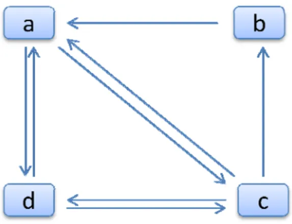
(39) . players is larger than or equal to the minimum similarity threshold, the two players can be grouped into a cluster; otherwise, they are not grouped. After this phase, all players could be grouped into several clusters based on their similarities in the feature table.. 4.5. Phase 4: Games Ranking. In our study, the voting concept of the novel PageRank algorithm is applied to rank all game items in a player group. The main idea is that links and pages in the voting concept can be mapped to players and game items, respectively. For example, assume a click sequence is <abc>, which represents that game item b is clicked after game item a has been clicked, and game item c is clicked after game item b has been clicked. In this study, the relationship of the continuous two items in a sequence is regarded as a link. There are thus two links in the sequence, ab and bc. For now, assume a player group includes three players, player 2, player 3, and player 4, and their click sequences are <cacda>, <acdac>, and <dadcba>. By using the above process, the seven links, ad, ac, ba, ca, cd, da, and dc, can be found from the three sequences, and the link relationship of game items can be represented as Figure 2 by the seven links.. 31 .

(40) . Figure 2: The link relationship of game items for this example.. Based on Figure 2, the adjacency matrix can be built that is shown in Table 5.. Table 5: The adjacency matrix for this example. a. b. c. d. a. 0. 0. 1. 1. b. 1. 0. 0. 0. c. 1. 1. 0. 1. d. 1. 0. 1. 0. To calculate the ranking value, the reverse adjacency matrix is then obtained, as shown in Table 6.. Table 6: The reverse adjacency matrix for this example. a. b. c. d. a. 0. 1. 1/3. 1/2. b. 0. 0. 1/3. 0. c. 1/2. 0. 0. 1/2. d. 1/2. 0. 1/3. 0. 32 .

(41) . In this way, we can get the vote number of links between game items. By using the PageRank algorithm, the page rank (PR) value of each game item can be found. Here, the initial damping factor is 0.85. As definition 17 shows, the page rank (PR) value of item a can then be calculated as (1-0.85) + PR (b) + PR (c) / 3 + PR (d) / 2, which is 0.331436. All the other game items in the cluster can be similarly processed in the same way. After this process, all the game items in the player cluster are listed in descending order of the calculated PR values of the items, as shown in Table 7. This process can be carried out for the other player clusters to obtain their ranking lists.. Table 7: The page rank values of all game items for this example.. 4.6. Game Item. PR Value. a. 0.331436. c. 0.288959. d. 0.260232. b. 0.119372. Games Recommendation. In the offline part, an effective recommendation strategy is designed to provide the top-k game items for players based on the ranking lists and clusters. The strategy that is adopted depends on whether the player the player is new or not. If they are new, then there is no playing game items information for the player in the website log file, and thus it is not easy to know which cluster is the player should be in. For this reason, 33 .

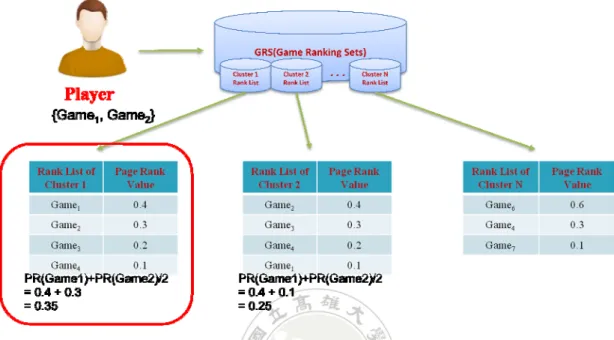
(42) . when a player originally registers a new account on the online game website they need to complete a questionnaire about their game item preferences. Based on the result of this, the new player’s preferred game items can be used to find the ranking list with the largest average PR value for all clusters, and then the top-k game items in the list with the largest average PR value are selected and provided for the new player. On the other hand, if the player is an experience one, then the top-k game items in the list for the cluster in which he or she belongs to are selected and provided to him or her. For example, in Figure 3, assume one new player’s preferred game items include two game items, Game 1 and Game 2, and there are N player clusters and their corresponding ranking lists. Take the first cluster as an example. The ranking list of the first cluster includes four game items, Game 1, Game 2, Game 3, and Game 4, and the PR values of these are 0.4, 0.3, 0.2, and 0.1, respectively. Next, the new player’s preferred game items are Game 1 and Game 2, and the PR values of these in the first cluster are 0.4 and 0.3. The average PR value of the first cluster for the new player can then be calculated as (0.4 + 0.3) / 2, which is 0.35. The above process is carried out for the other player clusters in Figure 3. Finally, the ranking list for the cluster with the largest average PR value is selected, and the top-k game items in the selected list are provided for the new player. On the other hand, assume the player is an experience one, and the player belongs to the second player cluster. As Figure 3 shows, the ranking list for the second cluster 34 .

(43) . includes four game items, Game 2, Game 3, Game 4, and Game 1, and then the top-k game items in the ranking list are selected and provided to this player.. Figure 3: The process of calculating the average PR value of each cluster.. 35 .

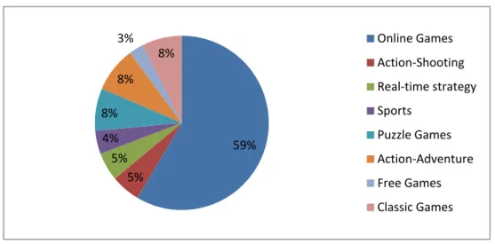
(44) . Chapter 5 Experimental Evaluation A series of experiments were conducted to compare the different recommendation lists obtained from multi-feature mining and clustering mining with different parameter values. Both processes were implemented in Delphi XE and executed on a PC with 2.4 GHz CPU and 4 GB memory.. 5.1. Experimental Dataset. In order to show practical results of the recommendation list system, a real dataset from an online game system is used in the experiment. Based on the goal and scope of this work, we included PC games data from 2011 to 2012, giving a total of 533 game items. These were then divided into eight kinds of games, with online games being the majority, with a total of 312, followed by the action-adventure category, with a total of 45. Details of this are shown in Figure 4.. 36 .

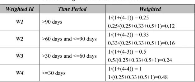
(45) 3%. Online Games 8%. Action‐Shooting. 8%. Real‐time strategy Sports. 8% 4% 5% 5%. Puzzle Games. 59%. Action‐Adventure Free Games Classic Games. Figure 4: The classification of the game items.. The system then collected a variety of statistics from the players’ historical record, as shown in Table 8.. Table 8: Statistical data collected from the players’ historical records. Items. Count. Number of players Total number of games. 2,882 554. 5.2 Evaluation on a Real Dataset The main goal of the experimental analysis was to verify the effectiveness of the system using a real dataset. The forecast results to measure a player's level of interest were used to set the optimal cluster size. First, we set a weight table in the feature mining phase, and distinguished between the different time periods in order to produce the relative weights, as shown in Table 9, based on the method described in definition 5.. 37 .

(46) . Table 9: Weights of the different time Periods. Weighted Id. Time Period. Weighted. W1. >90 days. 1/(1+(4-1)) = 0.25 0.25/(0.25+0.33+0.5+1)=0.12. W2. >60 days and <=90 days. 1/(1+(4-2)) = 0.33 0.33/(0.25+0.33+0.5+1)=0.16. W3. >30 days and <=60 days. 1/(1+(4-3)) = 0.5 0.5/(0.25+0.33+0.5+1)=0.24. W4. <=30 days. 1/(1+(4-4)) = 1 1/(0.25+0.33+0.5+1)=0.48. Next, Table 10 showed the number of features in the two kinds of databases, transaction and sequence, and the execution time of finding the two kinds of patterns in databases under different minimum support thresholds. Note that the FTDB and FSDB represented the numbers of features in a transaction database and a sequence database, respectively. Table 10: Numbers of features and consume time along with different thresholds. Min_Supp. FTDB. FSDB. Total. Execution Time (Sec.). 0.0600. 0. 0. 0. 5.689. 0.0400. 0. 0. 0. 5.680. 0.0200. 2. 2. 4. 5.717. 0.0100. 8. 8. 16. 6.321. 0.0080. 10. 11. 21. 6.773. 0.0060. 16. 17. 33. 8.262. 0.0040. 26. 28. 54. 11.148. 0.0039. 26. 28. 54. 12.158. 0.0038. 26. 28. 54. 13.116. 0.0037. 30. 30. 60. 13.427. 0.0036. 31. 33. 64. 14.079. 0.0035. 31. 33. 64. 14.257. 38 .

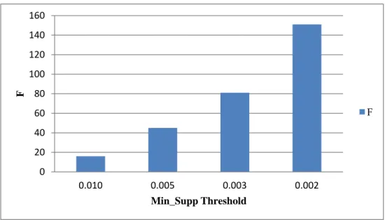
(47) . 0.0034. 31. 34. 65. 14.293. 0.0033. 33. 37. 70. 15.186. 0.0032. 36. 39. 75. 17.490. 0.0031. 38. 42. 80. 18.005. 0.0030. 38. 43. 81. 19.869. 0.0029. 40. 46. 86. 20.995. 0.0028. 40. 49. 89. 21.014. 0.0027. 44. 54. 98. 23.318. 0.0026. 47. 56. 103. 24.695. 0.0025. 47. 56. 103. 24.705. 0.0024. 52. 62. 114. 29.617. 0.0023. 58. 68. 126. 34.560. 0.0022. 62. 77. 139. 37.263. 0.0021. 65. 84. 149. 40.118. 0.0020. 66. 85. 151. 43.006. From Table 10, it could be observed that the number of features increased, and the consume time also increased when the minimum support threshold decreased. In the later experiment, the four minimum support threshold values, 0.01, 0.005, 0.003 and 0.002 were selected to evaluate the difference degree of recommended games in comparison with the baseline list that was consists of a set of popular games. The reason for this is that it had obviously gaps in the numbers of the features for the four threshold values, as shown in Figure 5. Note that the variable, F, represented the summation of frequent itemsets and sequential patterns. . 39 .

(48) 160 140 120. F. 100 80 F. 60 40 20 0 0.010. 0.005 0.003 Min_Supp Threshold. 0.002. Figure 5: Comparison the results with different min_supp thresholds. Next, Figure 6 evaluated the number of groups under different minimum similarity threshold values, such as 20%, 30%, 40%, 50% and 75%. As shown in Figure 6, when the threshold is set at 40%, the maximum group value of 66 could be obtained, and when the threshold is set at 20%, the minimum group value of 1 was obtained. Hence, the three minimum similarity threshold values, 20%, 30% and 40%, were selected to evaluate difference in top-k recommended games between the list of recommended. Clustering Count. games generated by our mechanism and the other list consisting of popular games.. 70 60 50 40 30 20 10 0. Clustering Count(min_supp=0.010) Clustering Count(min_supp=0.005) Clustering Count(min_supp=0.003) 20% 30% 40% 50% 75% Minimum Similarity Threshold. Clustering Count(min_supp=0.002). Figure 6: Comparison of the results with different similarity thresholds. 40 .

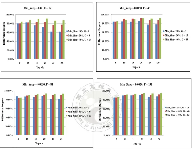
(49) . Finally, Figure 7 showed the differences in top-k recommended games between the list of recommended games generated by our mechanism and the other list consisting of popular games under different minimum support threshold values. Min_Supp = 0.0050, F = 45. Min_Supp = 0.01, F = 16 100.00%. 80.00% Min_Sim= 20%, G = 1. 60.00%. Min_Sim = 30%, G = 3 Min_Sim = 40%, G = 13. 40.00%. Difference Degree. Difference Degree. 100.00%. 80.00% Min_Sim= 20%, G = 2. 60.00%. Min_Sim = 30%, G = 13 Min_Sim = 40%, G = 43. 40.00%. 20.00%. 20.00%. 0.00%. 0.00% 5. 10. 15. 20. 25. 5. 30. 10. Min_Supp = 0.0030, F = 81. 20. 25. 30. Min_Supp = 0.0020, F = 151. 100.00%. 100.00%. 80.00% Min_Sim= 20%, G = 3. 60.00%. Min_Sim = 30%, G = 37 Min_Sim = 40%, G = 66. 40.00%. Difference Degree. Difference Degree. 15. Top - k. Top - k. 20.00%. 80.00% Min_Sim= 20%, G = 13 Min_Sim = 30%, G = 48 Min_Sim = 40%, G = 63. 60.00%. 40.00%. 20.00%. 0.00%. 0.00% 5. 10. 15. 20. 25. 30. 5. Top - k. 10. 15. 20. 25. 30. Top - k. Figure 7: The different clustering counts compare the recommended degree results.. As the figures showed, it could be observed that the difference between two lists was obviously different when the number of features increased. The reason for this is that the proposed mechanism could effectively distinguish difference between players according to their playing game features. Based on our proposed mechanism, more. 41 .

(50) . potential popular games in a game platform could be provided players in comparison with the intuition method, the list of popular games. In addition, the results showed the difference of the two lists was the largest under the top-20 recommended games. Thus, the suitable k value on our collected dataset might be set at 20. Overall, our proposed mechanism could generate a list of potential games by players’ features information in comparison with the list of intuition popular games.. 42 .

(51) . Chapter 6 Conclusions and Future Works General recommendation methods first need to set up the evaluation criteria, and then users give scores to items based on these. Based on these, the users are then put into several groups. However, the criteria that should be used are often not intuitive to users. In this thesis we thus develop a recommendation mechanism which does not need the users to carry out any rating actions, and instead is based on extracting various features from the users’ historical data. In particular, the Apriori-based weighted data mining method is used to identify common features of the game items in different groups of players. In addition, the CAST clustering method is adopted to put players into several groups. The PageRank algorithm is also applied to the game items, and thus those in the same group can be ranked in descending order of their ranking values. In this way, the system matches the ranked game lists of groups of similar players, and thus can help players to find games that they are more likely to be interested in. Experiments were carried out in this work to measure the performance of the system with regard to the use of multi-feature mining, and the results show that it can achieve good results. In future work, we will gather more data to find more features information, and. 43 .

(52) . continue to apply the concepts of different technologies to the game recommendation system, such as fuzzy or ontology approaches. In addition, we will also undertake a more complete experimental study, including adjusting the weighted parameters of different time periods, and then comparing the accuracy comparison of the resulting recommended results.. 44 .

(53) . References [1] A. Ben-Dor and Z. Yakhini, "Clustering gene expression patterns," Journal of Computational Biology, Vol. 6, 1999, pp. 281-297 [2] C. Ting-Kuang, "A multi-criteria Game Recommendation System Based on User Experience," National Taiwan University, 2008. [3] J. L. Herlocker, J. A. Konstan and L. G. Terveen, "Evaluating collaborative filtering recommender systems," ACM Transactions on Information Systems, Vol. 22(1), pp.5-53, 2004. [4] L. Page, S. Brin, R. Motwani, and T. Winograd, "The PageRank citation ranking: bringing order to the web," Technical Report, Stanford Digital Libraries Technologies Project, 1998. [5] N. Belkin and B. Croft, "Information filtering and information retrieval," Comm. ACM, vol. 35, no. 12, pp. 29-37, 1992. [6] R. Agrawal, T. Imielinski, and A. Swami, "Mining association rules between sets of items in large databases," In proc. of the ACM SIGMOD Conference on Management of Data, 1993, pp. 207-216. [7] R.. Baeza-Yates. and. B.. Ribeiro-Neto,. "Modern. information. retrieval,". Addison-Wesley, 1999. [8] R. Paul and R. V. Hal, "Recommender systems," Communication of ACM, vol. 40, 45 .

(54) . no. 3, pp. 56-58, 1997. [9] T.P.Hong, H.Y.Lee and G.C.Lan, “An efficient upper-bound model for mining weighted sequenctial patterns,” The 23rd International Conference on Information Management, pp. 197-198, 2012. [10] U. Yun, “On pushing weight constraints deeply into frequent itemset mining,” Intelligent Data Analysis, Vol. 13, No. 3, pp. 359-383, 2009. [11] U. Yun and J.J. Leggett, “WSpan: weighted sequential pattern mining in large sequence databases,” The 3rd International IEEE Conference on Intelligent Systems, pp. 512-517, 2006.. 46 .

(55)