An Adaptive Concentric Clustering Scheme for
Energy Efficient Routing in Wireless Sensor
Networks
Yih-Chuan LinDepartment of Computer Science and Information Engineering, National Formosa University, Yunlin, Taiwan
63201. [email protected]
Kai-Wei Jiang
Institute of Electro-Optical and Materials Science, National Formosa University, Yunlin, Taiwan 63201.
Abstract―This paper presents an adaptive
concentric clustering scheme to construct a routing topology which can reduce the transmission distance between nodes in a wireless sensor network for gathering sensory data from a base station. Depending on the current location of base station, the proposed algorithm can divide the set of network nodes into several concentric clusters and establish individual routing chain within each cluster such that the transmission distance between neighboring nodes on the chain is reduced. In addition, the proposed algorithm can automatically select appropriate cluster heads for the concentric clusters according to the number of sensor nodes remained so far in each cluster, which can also shorten the transmission distance between neighboring cluster heads. By computer simulation, the results show that the proposed algorithm performs better than other similar protocols in terms of energy save and lifetime increase capabilities for wireless sensor networks with random deployment of sensor nodes.
Index Terms― wireless sensor networks;
PEGASIS; concentric clustering; energy saving.
I. Introduction
Recent advances in wireless communications and micro-electro-mechanical systems (MEMS) have enabled the drastic progress of sensor networks technologies. By these small and low-cost sensory devices, which are equipped with sensing, computation and wireless communication capabilities, it becomes easier to construct a wireless sensor network (WSN) over physical spaces for monitoring environments, vehicles or
buildings etc. Most applications in wireless sensor network are targeting for gathering sensory data in real-time from some habitat environments, military battlefields, and humans for data managements and decision making for physical phenomena. Unlike other types of network, wireless sensor network has the capabilities of self-organization and automatic data collection of environment information. There are different developments on sensor networks in literature, such as the design of energy efficiency routing algorithm, sensor network coverage, internet security, object tracking and hardware architecture design. Interested readers can refer to [2][6] for more in-depth information.
Due to the natures of small size and simple design, these sensor nodes are constrained to have limited battery power, memory storage and computing power. Besides, replenishment of battery power resource should be a difficult job for a network composed of a large number of sensor nodes spread over a wide physical space. Energy-efficient routing protocol design is one of the most important problems in the networks of battery-powered wireless sensor nodes [11].
Intuitively, the amount of energy consumption does bear directly on radio transmission distance between sensor nodes. Many energy-efficient routing algorithms in literature for WSNs, such as Low Energy Adaptive Clustering Hierarchy (LEACH) [12], Power-Efficient GAthering in Sensor Information Systems (PEGASIS) [9] and Enhanced PEGASIS (EP) [4], have used the principle of shortening radio transmission distance
during the discovery of routes for data forwards. In LEACH, the network uses random-clustering scheme to divide itself into a set of sub-networks (called clusters) and collect sensory data locally within each cluster. It can decrease both the frequency and distance that sensor nodes need to transmit to base station directly. But it has a critical problem that the clusters may possess significantly different number of nodes. The different cluster size problem will lead to some nodes spend more energy than the nodes in other clusters. Under such unbalance energy consumption situation, it will shorten the network lifetime. Moreover, it may also cause that no cluster head was selected due to the usage of random probability to determine the cluster head [3][8][12].
In PEGASIS, the network acts as a large cluster and all nodes in the network are formed into a form of chain for transmission. The transmission distance between neighboring nodes on the chain is much reduced and only one head-node is required to transmit data to the base station. For these reasons, PEGASIS can save more energy than LEACH. However, PEGASIS has the redundant data transmission problem, which would waste extra energy consumption for delivery in the circuitous routing chain to the base station [4]. Besides PEGASIS uses a greedy algorithm to construct the routing chain that would result in relative large transmission distance between some neighboring nodes on the chain. This situation would make these nodes died faster than other nodes and then shorten the network lifetime. Furthermore, the long transmission delay with which the data travels to the base station via the chain routing topology is another problem in PEGASIS [3][4][9].
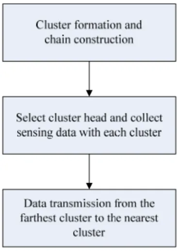
Afterward, EP uses concentric clustering scheme to mitigate the redundant energy consumption of PEGASIS. From the base station, EP uses concentric clustering scheme to evenly divide the network nodes into several clusters with identical cluster size. Next, EP performs similar work as PEGASIS to construct chain in each cluster. The data transmission across clusters is performed in the order from the farthest cluster to the nearest cluster, and finally to the base station. With this mechanism of data transmission, EP [4] can
decrease redundant data transmission. However, EP has the same problem that transmission distance between nodes is too long whether in between cluster heads or general nodes within single cluster. One of the reasons is that the starting node in the chain construction and the selection rule of cluster heads are not suited for the network topology. EP uses greedy algorithm to perform chain construction, which starts at the farthest node from the base station in each cluster and progressively connects the remaining nodes one at a time using the greedy policy of shortest distance. Owing to the fixed selection rule, the starting node selected is not always at a good start point for chain construction within a cluster. Therefore, it may still result in relatively long transmission distances between neighboring nodes and redundant transmission phenomenon and thus makes these nodes dead rapidly.
In this paper, the main design concept is focused on the time-driven model [3][5][10]. We propose an algorithm “Boundary First PEGASIS” that can adapt the construction of routing topology by taking into account the position of base station and the current number of active nodes in each cluster. The approaches for the adaptability are to use vector projection approach which considering the location of base station, for constructing the network topology, and to design cluster head selection rule, which depend on the number of active nodes in the WSN, to construct the inter-head nodes data routes.
The system model on which the proposed algorithm is based can be represented as shown in Figure 1. When the sensor nodes have been deployed, the base station starts to broadcast an initial message to collect the individual status information of all nodes, and then all nodes reply responses respectively. Next the base station performs the cluster and chain formation and broadcasts the result to the network. Further, all nodes that receive the information from the base station can proceed their own initial setting to establish the initial routing topology, such as obtaining its cluster number and its order number on the chain for constructing communication path. After a certain period of time, the base station starts to broadcast the “data collect” command, and then
all nodes start to collect sensing data for the base station. This process can be regard as a round (fixed time period) and the base station has to issue the data collect command every round of time. Once some nodes are died (the data collection process is failure), the base station can become aware of this situation through time out and then to broadcast Maintenance message. All nodes start to check whether its neighbor died or not and reconstruction the communication path. After that, all nodes proceed with data forwarding.
The remainder of this paper is organized as follows: Section 2 is devoted to the proposed algorithm. Section 3 provides the simulations results and evaluates the proposed algorithm. Finally, concludes are given in Section 4.
Figure 1 System operation process of BFP.
II. The Proposed Algorithm
The proposed algorithm has following assumptions:
y Sensor nodes know their own positions in the monitoring field.
y Sensor nodes can adjust its radio power level to communicate with other nodes or base station. y The lower communication protocols of the WSN
considered have no automatic acknowledge scheme. Reliable data transmission can be performed by the routing protocol itself if
require.
Figure 2 shows the flowchart of the proposed algorithm. It is named after PEGASIS to be Boundary First PEGASIS (BFP) due to its natures like PEGASIS. In this section, we describe the complete works that are needed to achieve the target requirements.
For the ease of explanation, Table 1 defines the notations that are used in this paper.
Let us first discuss that how the position of base station affects the routing topology to be constructed.
Table 1 Definition of notations Notation Definition
i
s Sensor nodes in the network,
1, 2,...,
i= n
S Node set; S={ ,s s1 2,...,sn}
BS Base station
( ,i )
d s BS The distance between node si and
BS ( )i C s Cluster number of s , i max ( )i 1, 2,..., C s = c c CS Cluster set; max { ( ) }; 1, 2,..., c CS = ∈s S C s =c c= c
Li(r) Cluster head in cluster i at the r-th
round; the corresponding order number on the chain would be cluster head ( )
i
T r Total number of nodes in cluster i at the r-th round
A(r) Total number of nodes in the network at the r-th round
( )
PN r Total number of clusters in the network at the r-th round
(xM,yM) The location of center point (M) of the sensor field
(xB,yB) The location of Base station
( , )
i i
s s
x y The location of node s i ( )
i
O s Order number of nodes on the chain in the cluster i; s∈CSc
A. Impact of the Location of Base station and Data Routing
t
Figure 2 Flowchart of BFP.
the lifespan of the WSN can be maximized has ever been addressed and proved to be a NP-complete problem under some pre-specified conditions [1]. Researchers have used integer programming, computational geometry, local search and greedy heuristics to find sub-optimal solution [7].
The base station can be regarded as a member in the network, because all nodes have to transmit data to the base station. Apparently the energy consumption of nodes has indirect bearing on the location of base station; in other words the location of base station has impact on the data routing. We randomly deploy nodes to simulate EP and use different markers/colors to denote different clusters as show in Figure 3. To examine the network topology in cluster 2 (blue marker) in Figure 3 (a) and (b), we can see that under the same node distribution, once the location of base station is moved to a new place, the shape of cluster formation or network topology is changed correspondently. These variations can affect the performance of a routing algorithm. From the viewpoint of routing design, only uses concentric clustering is not enough. Our purpose is to construct a good network topology that can adapt with different locations of base station, as the example shown in Figure 4.
Specifically, for the example in Figure 5, we let all nodes in a cluster to project their position vectorssv onto a principal vector (i vv ). For each cluster of nodes, the principal vector is defined as follows,
Figure 3 Illustration of the influence the location of base station on data routing
Figure 4 A Good network topology when confront with different environments.
⎪ ⎪ ⎩ ⎪⎪ ⎨ ⎧ − = = = otherwise y x y if y x if x v M M a M a M ) , 1 ( 0 ) , 0 ( 0 ) 0 , ( v (1)
where xa and ya represent the x- and y-components
of another vector av that points to the base station from the position (xM, yM), i.e.,
av=(xB −xM,yB−yM) (2)
vv vv
av
i sv
Figure 5 Using projection approach to construct the chain.
To construct the chain of nodes, the order of nodes on the chain is arranged in consistent with the order of the corresponding projective values on the vector vv as shown in Figure 5 (b). Apparently, the chain construction process would changes with the positions of the base station; the network topology can be controlled to adapt to the different location of base station problem and can avoid the irregular topology.
B. The Cluster Head Selection Rule
Because cluster heads have to spend more energy than general nodes, therefore all nodes are taking turns to be cluster head and consume energy equally. A simple cluster head selection rule in EP which can achieve the purpose is
) ( mod ) (r r T r Li = i (3) It would perform well when the number of active nodes is same in each cluster, as shown in Figure 6. However, when nodes become inactive due to drained out of battery energy or other reasons, the cluster sizes among the clusters would become different and cause the different cluster size problem, which lead to a irregular forwarding path and thus more energy dissipation. The maximal transmission distance can be the length/width of the network field in the extreme case. Apparently it is serious energy consumption.
Figure 6 Illustration of the different cluster size problem.
Therefore, we propose a selection rule for cluster heads that can adapt to the different number of active nodes in clusters. This rule is called average-cluster-size based rule (ACSB for short) and (4) and (5) define its operation. In order to keep the rotation feature and maintain the
transmission consistently, we let the average of the cluster size over all the clusters to control the behavior of the selection rule. The purposes of ACSB are to reduce the transmission distance between cluster heads and let all nodes have chance to be cluster head. ) ) ( ) ( ( mod ⎥⎦ ⎥ ⎢⎣ ⎢ = r PN r A r L (4) ) ( 1 ) ( ) ( ) ( ⎩ ⎨ ⎧ ≥ − < = r T L r T r T L L r L i i i i (5)
Eq. (5) is used to see if the number of node in the cluster is less than the order number of the next cluster head. In this case, the order number of cluster head Li(r) is set to Ti(r)-1. Let us see
an example in Figure 7, in the (r+1)-th round (Figure 7 (b)), cluster 2 can not select a suitable node to be cluster head because of the fewer number of nodes than the average cluster size. At this time, nodes can use equation (5) to select the last sensor node in the cluster as the cluster head in this round.
⎣27/5⎦=5
⎣27/5⎦=5 ⎣27/5⎦=5
Figure 7 Illustration of the operation in ACSB.
C. BFP: Boundary First PEGASIS
Our WSN model requires doing the following tasks of BFP for constructing a routing topology. y Cluster and chain formation
In this phase, the tasks about cluster and chain formation are computed by the base station. After the base station collects the individual status information of all nodes deployed in the monitoring space, the base station needs to do the clusters and chains construction task below:
Algorithm 1: Cluster formation
Input: Nodes s1,s2,...,sn and cmax
Output:C(si); i=1,2,...,n
1. Use the Euclidean distance formula to calculate: ) , ( ),..., , ( ), , ( 1 2 2 1 d s BS d d s BS d d s BS d = = n = n
and store them in a distance table.
2. Sort the distance table and classify it into cmaxcluster
sets which each cluster has ⎥ ⎥ ⎤ ⎢ ⎢ ⎡ max c n nodes.
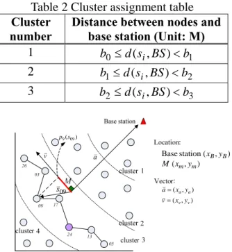
3. For each cluster i, the base station needs to determine a pair of cluster boundary distance value: bi−1and bi. Hence for all cluster sets together, there exists a sequence:{ , ,..., , } max 1 max 1 0 b bc bc b − .
These results can be tabulated as a cluster assignment table as like Table 2. Through base station to broadcast the cluster assignment table and the location information of the base station, each receiving node can realize its cluster number. Further, according to the location information of nodes, the base station can construct the relative localization and center point of the sensor field, as shown in Figure 8.
Table 2 Cluster assignment table Cluster
number
Distance between nodes and base station (Unit: M) 1 b0 ≤d(si,BS)<b1 2 b1≤d(si,BS)<b2 3 b2 ≤d(si,BS)<b3 vv av Basestation (xB,yB) ) , (xm ym M ) , (xaya av= ) , (xv yv vv= 09 sv ) (09 9s p
Figure 8 Illustration of projection approach to construct the chain.
For each cluster set CSc where
} ) ( {s SC s c
CSc = ∈ = , We can use vector
projection approach to perform chain construction in each cluster which can avoid the problem in EP and shorten the transmission between nodes. The chain construction is also performed by the base station and does following steps through algorithm 2:
Algorithm 2: Chain construction
Input: All cluster sets CSc; c=1,2,...,cmax.
Output:Oc(s),s∈CSc,c=0,1,2...,cmax.
1. Calculate a spatial vector av which connect the center point M with the base station and calculate the vertical vector vv which perpendicular to vector av.
2. For each node in CSc, the base station calculates a vector svi which connects the center point M to node
i
s . Next, uses equation (6) to calculate the pi(si)which
indicates the projection of svi onto vv. v v s s pi i iv v v ⋅ = ) ( (6) 3. For the cluster set CSc, collect all the projection values in the cluster as a projection set
)} ( ),..., ( ), ( { 1 1 2 2 c c CS CS c p s p s p s P = .
4. Sort Pc and for each node in CSc, assign an appropriate integer from {0,1,2,...,CSc −1} to Oc(s),
c CS s∈ such that Oc(si)<Oc(sj) if ) ( ) (si p sj
p < for any pair of different nodes j i c j i s CS s s s, ∈ ; ≠ .
For example, as shown in Figure 8, let us look at node 09 in cluster 3: the base station calculates vector sv09and )p(s09 to indicate the projection length (red line) of sv onto 09 vv . Other nodes in the cluster are treated with the same operation. All results of operation can be tabulated as a table. Next, sort the table with column P as like shown in Table 3. The order c of nodes in the Table 3 is the result about the order of nodes on the chain, as shown in Figure 8.
After these steps, the base station broadcasts the
results about the sequence:
} , ,..., , { max 1 max 1 0 b bc bc b
− and the sorted P to c
each cluster sequentially. When a node receives these information, it can set related parameters for constructing routing. These parameters are
needed to maintain by each node, as tabulated in Table 4. For each receiving node s in the i cluster c uses Algorithm 3 to set related parameters.
Table 3 Sort the projection length record with columnP 3 i s ( , ) i i s s y x P 3 05 (100,34) -46.7 13 (94,50) -31.1 24 (87,56) -21.9 17 (61,68) 4.9 09 (51,85) 24.0 03 (41,85) 31.1 26 (46,107) 43.1 Table 4 Maintain parameters for a node Variables Definition
num
C Cluster number
num
O Order number on the chain
L
neighbor _ Left-sided neighbor which its order number is Onum−1
R
neighbor _ Right-sided neighbor which its order number is Onum +1
CZ Cluster size of itself; initial
value is Pc
TN Total number of nodes in the
network; initial value is n
TC Total number of clusters in the
network; initial value is Cmax
Li(r) Cluster head in cluster i at the
r-th round; the corresponding order number on the chain would be cluster head. The first time to receive “data collect” command, Li(r) = 1
Algorithm 3: Set related parameters for constructing routing Input: { , ,..., , } max 1 max 1 0 b bc bc b
− , sorted Pc and the location
of base station
Output: Each node have to set parameters such as num
C , Onum, neighbor _L,neighbor _R, and CZ.
1. Sets its cluster number. If bk−1 ≤d(si,BS)<bk, then sets Cnum =k.
2. Sets Onum according to the index from
} 1 ,..., 2 , 1 , 0
{ Pc − in the Pc. Then sets CZ = Pc . 3. Constructs/Sets communication route and collect the location information of neighbor nodes:
Switch (Onum)
Case 0: with the right-side neighbor node (order
number = Onum+1). Sets neighbor _R.
Case CZ-1: with the left-side neighbor node (order
number = Onum−1). Sets neighbor _L.
Default: with the two-sided neighbor nodes (order
number = Onum+1 and Onum−1 ). Sets
R
neighbor _ and neighbor _L.
This information has aids for maintaining an accuracy data transmission routes. In addition, each node can adjust a suitable power level while transmitting sensing data according to the location information of its neighbor nodes. y Data forwarding
After base station broadcasts the “data collect” command which includes values in variables TN, TC and r. The data collection process is performed first by all clusters concurrently, and then cluster heads transmit their own data orderly from the farthest cluster to the nearest cluster, which is similar to EP. For the ease of discussion, the data forwarding can be divided into two parts: the process of data transmission only happened within the cluster, called intra communication, whereas the data transmission among clusters is called inter communication. The intra communication for each cluster performs Algorithm 4:
Algorithm 4: Intra communication
Input: Data collect command,TN ,TCand r.
Output: Aggregation data
1. Update Ti(r)=CZ;A(r)=TN;PN(r)=TC
2. For each node in the c-th cluster, to use the cluster selection rule to calculate Lc(r) in each round. 3. For each cluster i,
If Lc(r)≠Onum
Performs general node data collect procedure, as shown in Figure 9.
else
Performs cluster head data collect procedure, as shown in Figure 10.
Switch (Onum)
Case 0:
Initiates a counter: counterinter =0. 1
inter inter= counter +
counter .
Transmits counterinter and sensing data to
R
neighbor _ .
Case CZ−1:
Initiates a counter: counterinter=0. 1
inter inter= counter +
counter .
Transmits counterinter and sensing data to
L
neighbor _ .
Default: If Lc(r)>Onum
Waits to receives counterinter and sensing
data from neighbor _L.
1
inter
inter = counter +
counter .
Then to perform data fusion and transmits
inter
counter and data to neighbor _R.
else
Waits to receives counterinter and sensing data
from neighbor _R.
1
inter inter= counter +
counter .
Then to perform data fusion and transmits
inter
counter and data to neighbor _ . L
End if
Figure 9 General node-data collect procedure.
1. Switch (Onum) Case 0 :
Receives counterinter and sensing data from R
neighbor _ , and then to perform data fusion. 1
_temp= counterinter+ CZ
Case CZ−1:
Receives counterinter and sensing data from L
neighbor _ , and then to perform data fusion. 1
_temp= counterinter+ CZ
Default:
Receives counterinter and sensing data from R
neighbor _ .
inter _temp counter
CZ =
Receives counterinter and sensing data from L
neighbor _
inter _
_temp CZ temp counter
CZ = +
Then performs data fusion. 2. If CZ≠CZ_temp
temp CZ
CZ= _
Transmits CZ to its two-side neighbors End if
When a node receives CZ , it has to update CZ and transmits it to its neighbor. Therefore, each node can maintain accurate CZ sequentially.
Figure 10 Cluster head-data collect procedure. Through these steps, the cluster head can collect all sensing data in its cluster.
By Algorithm 5, cluster heads can relay all sensing data in the network to the base station and finish this round accordingly. Next all nodes wait to receive the data collect command and perform data collection. When the data collection process is failed (by timer expiration
in BS), it means the network has some nodes died. The base station can broadcast a Maintenance message to let all nodes to check whether its neighbor died or not and re-establish the broken link if necessary. For each receiving node in the c-th cluster, Algorithm 6 (shown on the next page) describes the process that need to be done for the case.
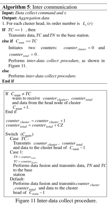
Algorithm 5: Inter communication
Input: Data collect command and r. Output: Aggregation data
1. For each cluster head, its order number is Lc(r)
If TC==1 , then
Transmits data,TCandTN to the base station.
else if Cnum ==TC
Initiates two counters: countercluster =0 and
0 =
total
counter .
Performs inter-data collect procedure, as shown in Figure 11.
else
Performs inter-data collect procedure.
End if
If Cnum≠TC
waits to receive countercluster, countertotal and data from the head node of cluster
1 + num C . End if 1 + = cluster cluster counter counter CZ counter
countertotal= total+
Switch (Cnum) Case TC :
Transmits countercluster, countertotal and data to the cluster head of Cnum−1 Case 1: total counter TN= cluster counter TC=
Performs data fusion and transmits data, TN and TC to the base
station Default:
Performs data fusion and transmitscountercluster
,countertotal and data to the cluster head of Cnum−1
Figure 11 Inter-data collect procedure. In Algorithm 6, the cluster number is needed to update for accurate data forwarding. Next the same principle of Step 2 in Cluster head-data collect procedure is used to inform other nodes in the cluster about the current cluster number. Afterward, the base station can collect data correctly until all
nodes died.
Algorithm 6: Topology maintenance
Input: Maintenance message.
Output: Update a accurate order number, neighbor _R
and neighbor _L.
1. To check its neighbor died or not.
Switch (Onum)
Case 0:
Performs intra communication (Algorithm 4) and inter communication (Algorithm 5).
Case CZ-1:
Performs maintain information procedure, as shown in Figure 12.
Sets neighbor _L.
Performs intra communication and inter communication.
Default:
Performs maintain information procedure Sets neighbor _L.
Sets a message: INFO_value = x and then transmits it to inform its right neighbor. Through this step, a node can realize itself is the boundary node (right side) or not. Therefore, if the cluster head in this round isLc(r)= CZ−1, the new boundary node has to replace to be the cluster head.
Performs intra communication and inter communication.
2. When a node receiving the inform message, to update its order number = Onum−INFO_value.
If its neighbor died, existing x death nodes which their order number<Onum , then its order number is reconstructed as Onum−x.
Constructs communication route and collects the location information of neighbor node with order number =Onum−1.
Figure 12 Maintain information procedure.
III. Simulation Result
In our simulation, the formal radio mode: first order radio model [4][9][12] is used to evaluate the performance. We simulated in a 120m x 120m sensor field and randomly deployed 144 nodes (in the EP and BFP, we divided the network into six clusters which each cluster had 24 nodes). The initial energy for each node is 0.5 J and 50 nJ for the energy consumption of transmitter/receiver unit; 100 pJ for the energy consumption of transmitter amplifier. The packet length is fixed at 2000 bits and needs 5 nJ for the energy consumption of data aggregation. In each simulated algorithm, we
perform 1000 times and average the results of the outcomes. If the base station is located at the fixed position (60,200), the simulation results are shown in Figures 13, 14 and 15.
Figure 13 shows the total residual energy in each round, we can see that BFP has the best performance in this environment and it performs better than EP and PEGASIS. Besides, we can see that when BFP uses the ACSB rule, it can obtain more energy conservation than the one that uses the original rule.
Figure 14 shows the average transmission distance of each node. Because the head node in PEGASIS transmits data to base station directly, therefore the average transmission distance of nodes at each round to routing data to the base station is shorter than BFP and EP. On the contrary in BFP, cluster heads transmits data to base station through multi-hop manner. For this reason, it can preserve more energy as shown in Figure 13.
Furthermore, Figure 14 also shows that the average transmission distance in EP is longer than BFP; it means the intra communication in EP is longer than BFP. Besides the amplitude of range in EP is higher than BFP; this implies the inter communication in EP is longer than BFP. Moreover, in this figure we can see that the curve of ACSB is smooth than the original rule. Apparently ACSB can adapt to the active nodes to shorten the transmission distance between cluster heads. Therefore ACSB can preserve more energy.
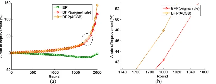
To compare with PEGASIS, we use equation (7) to examine the improvement rate of BFP and EP in each round. 100 ) ( ) ( ) ( ) ( = / − × r resd r resd r resd r rate P P E B (7)
where resdB/E(r) represents the total residual
energy in BFP/EP at r-th round; resdP(r)
represents the total residual energy in PEGASIS at r-th round. Figure 15 shows the result. As we see the improvement rate in BFP has about 43% in 1800 round; ACSB has about 48% in 1800 round. These simulation results have verified the facts that BFP can solve the problem in EP and that ACSB cluster head selection rules can outperform the selection rule in PEGASIS.
(a) (b)
Figure 13 Total residual energy of each node. We magnify partial (a) to (b).
(a) (b)
Figure 14 Average transmission distance of each node. We magnify partial (a) to (b).
(a) (b)
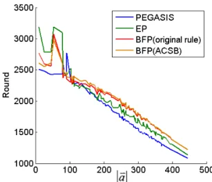
Next, we randomly test 100 different positions of base station in the considered space to gather sensory data for a fixed deployment of 144 sensor nodes and measure the network lifetimes (in terms of round). As like shown in Figure 16, these positions are restricted within in the red-square area. In such simulation environment, Figure 17 and 18 shows the first node die and all nodes die respectively, the horizontal coordinate represents the distance between different positions of base station and the center point of sensor filed. In the most cases, the performance of the proposed algorithm can perform better than EP and PEGASIS. However, according to our observation, the performance of the proposed algorithm decreases when the position is located within the sensor field. 1 B 1 av 2 B 2 av 3 av 3 B
Figure 16 Illustration of random deploy different position of base station.
Figure 17 The network lifetime when the first node die. The curves of the proposed algorithm are overlapped. Therefore, only three curves are displayed in this figure.
Figure 18 The network lifetime when the all nodes die. In order to display a clear result, so the improvement on the ACSB cluster head selection rule is not obvious (the curve of width is thick).
IV. Conclusion
In this paper, we propose schemes that can adapt the construction of WSN routing topology to the positions of base station and consumes energy conservatively when aggregating sensory data orderly within each cluster and across cluster heads. For different base station’s positions, the proposed algorithm can shorten the distance and control the network topology through the vector projection approach. When the numbers of active nodes among the clusters are different, the proposed head-node selection rule can adapt to this dynamic phenomenon and further prevent the extended crisscross transmission phenomenon. By simulation, the proposed schemes can be energy-efficient and be adaptive when confront with different position of base station.
Unavoidably, the transmission mechanism of concentric clustering scheme has a common problem, that is, nodes which are within the nearest cluster to the base station would exhausted more quickly due to their heavy multi-hop relays. A simple way to solve this problem is to change the location of base station periodically. In such situation, the proposed algorithm can be used adaptively for different base station placements.
REFERENCE
[1] A. Efrat, S. Har-Peled and J.S.B. Mitchell, “Approximation algorithms for two optimal
location problems in sensor networks,” 2005 2nd International Conference on Broadband Networks, vol. 1, pp.714-723, October 2005 [2] I.F. Akyildiz, W. Su, Y. Sankarasubramaniam
and E. Cayirci, “A Survey on Sensor Networks,” IEEE Communications Magazine, vol. 40 no. 8, pp.102-114, August 2002.
[3] J. N. Al-Karaki, A. E. Kamal, “Routing Techniques in Wireless Sensor Networks: A Survey,” IEEE Wireless Communications, vol. 11 no. 6, pp.6-28, December 2004.
[4] S. M. Jung, Y. J. Han and T. M. Chung, “The Concentric Clustering Scheme for Efficient Energy Consumption in the PEGASIS,” The ninth International Conference on Advanced Communication Technology, vol. 1, pp.260-265, February 2007.
[5] K. Holger, A. Willig, Protocols and Architectures for Wireless Sensor Networks, Chichester, England: Wiley, 2005.
[6] K. Romer, F. Mattern, “The Design Space of Wireless Sensor Networks,” IEEE Wireless Communication, vol. 11 no. 6, pp.54-61, December 2004.
[7] K. Akkaya, M. Younis, and M. Youssef, “Positioning of Base Stations in Wireless Sensor Networks,” IEEE Communications Magazine, vol. 45, pp.96-102, April .2007.
[8] C. M. Liu, C. H. Lee and L. C. Wang, “Distributed Clustering Algorithms for Data-gathering in Wireless Mobile Sensor Networks,” Journal of Parallel and Distributed Computing, vol. 67 no. 11, pp.1187-1120, November 2007.
[9] S. Lindsey and C. S. Raghavendra, “PEGASIS: Power-Efficient GAthering in Sensor Information Systems,” IEEE Aerospace Conference Proceedings 2002, vol. 3, pp.1125-1130, 2002.
[10] S. Tilak, Nael B. Abu-Ghazaleh and W. Heinzelman, “A Taxonomy of Wireless Micro-sensor Network Models,” ACM SIGMOBILE Mobile Computing and Communications Review, vol. 6 no. 2, pp.28-36, April 2002.
[11] S. Mahfoudh and P. Minet, “Survey of Energy Efficient Strategies in Wireless Ad Hoc and Sensor Networks,” IEEE Seventh International Conference on Networking, pp.1-7, April 2008.
[12] W. R. Heinzelman, A. Chandrakasan and H.
Balakrishnan, “Energy-efficient Communication Protocol for Wireless
Microsensor Networks,” IEEE Proceedings of the Annual Hawaii International Conference on System Sciences, pp.1-10, January 2000.