Fast Direct Solver for Poisson Equation in a 2D
Elliptical Domain
Ming-Chih Lai
Department of Applied Mathematics National Chiao Tung University 1001, Ta Hsueh Road, Hsinchu 30050 Taiwan
Received 14 October 2002; accepted 20 May 2003 DOI 10.1002/num.10080
In this article, we extend our previous work (M.-C. Lai and W.-C. Wang, Numer Methods Partial Differential Eq 18:56 – 68, 2002) for developing some fast Poisson solvers on 2D polar and spherical geometries to an elliptical domain. Instead of solving the equation in an irregular Cartesian geometry, we formulate the equation in elliptical coordinates. The solver relies on representing the solution as a truncated Fourier series, then solving the differential equations of Fourier coefficients by finite difference discreti-zations. Using a grid by shifting half mesh away from the pole and incorporating the derived numerical boundary value, the difficulty of coordinate singularity can be elevated easily. Unlike the case of 2D disk domain, the present difference equation for each Fourier mode is coupled with its conjugate mode through the numerical boundary value near the pole; thus, those two modes are solved simultaneously. Both second- and fourth-order accurate schemes for Dirichlet and Neumann problems are presented. In particular, the fourth-order accuracy can be achieved by a three-point compact stencil which is in contrast to a five-point long stencil for the disk case. ©2003 Wiley Periodicals, Inc. Numer Methods Partial Differential Eq 20: 72– 81, 2004
Keywords: fast Poisson solver; elliptical coordinates; compact scheme; symmetry condition
I. INTRODUCTION
Many physical problems involve solving the Poisson equation in two- or three-dimensional domains. For example, the projection method for the numerical solution of the incompressible Navier-Stokes equations requires solving the pressure Poisson equation. Very often, the problem we are interested in is no longer in a rectangular domain. For instance, many applications in the areas of meteorology, geophysics, and astrophysics involve solving a Poisson equation on a spherical geometry. Another example is for the micro-magnetics simulations. The dynamics of the magnetization distribution in the ferromagnetic material involves solving the Landau-Lifshitz equation. In [1], E and Wang have developed a simple projection method for the damping term, which requires to solve the heat equation with zero Neumann boundary
Correspondence to: M.-C. Lai (e-mail: [email protected])
Contract grant sponsor: National Science Council of Taiwan; contract grant number: NSC-90-2115-M-194-018
condition. If the ferromagnetic material has the shape of 2D or 3D elliptical geometries such as the one considered in [2], then an efficient Poisson-type solver on those domains is needed. This is exactly the motivation of our present work.
In [3], the author and his collaborators have developed a class of FFT-based fast direct solvers for Poisson equation in 2D polar and spherical domains. The methods have three major features, namely, the coordinate singularities can be treated easily, the resulting linear equations can be solved efficiently by existing fast algorithms, and the different boundary conditions can be handled without substantial differences. Besides, the method is easy to implement. In this article, we apply the similar idea to develop an efficient Poisson solver in a 2D elliptical region. Instead of solving the equation in an irregular Cartesian domain, we write the equation in elliptical coordinates. Our method relies on representing the solution as a truncated Fourier series, then solving the differential equations of Fourier coefficients by second- and fourth-order finite difference discretizations. Using a grid by shifting half mesh away from the pole and incorporating the derived numerical boundary value, the main difficulty of coordinate singu-larity can be elevated easily.
Although the present approach used in elliptical domain is similar to [3], the scheme for solving the reduced Fourier mode equation is completely different from the one used in polar domain [3]. For example, in the present formulation, the difference equation of the nth Fourier mode uˆ is coupled with its conjugate mode un ˆ through the inner numerical boundary value (the⫺n
numerical boundary value near the pole); thus, we need to solve those two modes altogether. This is in contrast to the polar coordinates case which the Fourier modes are fully decoupled thus can be solved independently. Another difference is that the present stencil for the fourth-order scheme is a three-point compact type, while the one used in [3] is a five-point long stencil. We will discuss those significant differences at appropriate places in the following sections.
II. POISSON EQUATION IN ELLIPTICAL COORDINATES
We consider the boundary value problem of Poisson equation in a 2D elliptical domain⍀ as ⭸2 u ⭸x2⫹ ⭸2 u ⭸y2⫽ f in⍀, (2.1) u⫽ g, or⭸u ⭸n ⫽g on⭸⍀, (2.2)
where the domain⍀ is described by ⍀ ⫽
再
共x, y兲冏
x2
共a cosh b兲2⫹
y2
共a sinh b兲2ⱕ 1
冎
. (2.3)The boundary of⍀, denoted by ⭸⍀, is an ellipse whose length of the major axis is 2a cosh b, the minor axis 2a sinh b, and the distance from the center to a focus is a. In order to solve the problem in the domain ⍀, we first transform the rectangular coordinates into the convenient elliptical coordinates and then rewrite the governing equations (2.1)–(2.2) in those new coor-dinates.
The Cartesian-Elliptical coordinates transformations are given by
x⫽ a cosh cos , y⫽ a sinh sin , (2.4)
so that the domain⍀ can be represented by 0 ⬍ ⱕ b, 0 ⱕ ⬍ 2. The coordinate curve ⫽ b generates the ellipse that is also the boundary of ⍀. Applying those coordinates to Eqs. (2.1)–(2.2), we have 1 h2
冉
⭸2 u ⭸2⫹ ⭸2 u ⭸2冊
⫽ f, 0⬍ ⱕ b, 0ⱕ ⬍ 2, (2.5) u共b,兲 ⫽ g共兲, or 1 h ⭸u ⭸ 共b,兲 ⫽ g共兲, (2.6)where the factor h2⫽ a2(sinh2 ⫹ sin2) is the Jacobian of the coordinates transformation (2.4). It is interesting to note that the Poisson equation (2.5) in elliptical coordinates seems to have a simpler form than the equation in polar coordinates [3]. The latter has an extra first-order derivative term for the Laplacian.
The equations (2.5)–(2.6) now become the boundary value problem in (, ) rectangular domain. The periodic boundary condition is imposed in direction and the value at ⫽ b is determined either by the Dirichlet or Neumann data. The remaining difficulty for solving the problem is lack of boundary value along the axis ⫽ 0; thus, some treatment must be taken in order to elevate this difficulty. This is the similar situation occurring in polar coordinates when the pole singularity is present at the origin. In the next section, we will extend the idea used for polar coordinates [3] to the elliptical coordinates. We first represent the solution as a truncated Fourier series and then solve the differential equations of Fourier coefficients by finite difference discretizations.
III. REDUCED FOURIER MODE EQUATION
Because the solution u is periodic in, we can approximate it by the truncated Fourier series as u共, 兲 ⫽
冘
n⫽⫺N/2 N/2⫺1 un ˆ共兲ein , (3.1)where uˆn共兲 is the complex Fourier coefficient given by
un ˆ共兲 ⫽1 N
冘
j⫽0 N⫺1 u共, j兲e⫺inj, (3.2)andj⫽ 2j/N, and N is the number of grid points along an ellipse. The above transformation between the physical space and Fourier space can be efficiently performed using the fast Fourier transform (FFT) with O(N log2N ) arithmetic operations.
Substituting the expansions of (3.1) into the equation obtained by multiplying h2on both
sides of (2.5), we derive the Fourier coefficients uˆn共兲, ⫺N/2 ⱕ n ⱕ N/2 ⫺ 1, satisfying the ordinary differential equation
d2 un ˆ d2 ⫺ n 2 un ˆ⫽ fˆ,n 0⬍ ⱕ b, (3.3) un ˆ共b兲 ⫽ gˆ ,n or uˆ⬘n共b兲 ⫽ gˆ.n (3.4) Here, fˆ() is the corresponding Fourier coefficient of the function hn 2f, and gˆ is the Fouriern coefficient of the function g (Dirichlet case) or hg (Neumann case). Those coefficients are defined in the same manner as Eqs. (3.1)–(3.2). Therefore, the problem of solving Poisson equation (2.5)–(2.6) now reduces to solving a set of Fourier mode equations (3.3)–(3.4).
In the following, we will develop the second-order centered difference and the fourth-order compact difference methods for the solution of Eqs. (3.3)–(3.4). Throughout this article, we adapt a grid similar to the polar coordinates case [3] as
i⫽ 共i ⫺ 1/2兲⌬, i⫽ 0, 1, 2, . . . , M, M ⫹ 1 (3.5) with the mesh width⌬ ⫽ 2b/(2M ⫹ 1). By the choice of ⌬, we have M⫹1⫽ b. We denote the discrete unknowns Ui ⬇ uˆn共i兲 and the values Fi ⬇ fˆ共n i兲. The second-order centered difference operators␦0and␦
2
to the first and second derivatives are defined by
␦0Ui⫽ Ui⫹1⫺ Ui⫺1 2⌬ , ␦ 2 Ui⫽ Ui⫹1⫺ 2Ui⫹ Ui⫺1 共⌬兲2 . (3.6) A. Second-order Scheme
Applying the centered difference operator ␦2to Eq. (3.3) directly, we obtain a second-order
scheme as
␦2
Ui⫺ n
2
Ui⫽ Fi, 1ⱕ i ⱕ M. (3.7)
In order to close the linear system of equations, two numerical boundary values U0
⬇ uˆn共⫺⌬/2兲 and UM⫹1 ⬇ uˆn共b兲 must be provided. The numerical boundary value UM⫹1is just
given by gˆ for the Dirichlet case. (In this and next subsections, we postpone the derivation ofn the inner numerical boundary value U0 to the last subsection.) For the Neumann problem,
however, the boundary value UM⫹1is not known; thus, the index of the unknowns must include
i⫽ M ⫹ 1. The Neumann data gives the condition UM⫹2⫺ UM
2⌬ ⫽ gˆ ,n (3.8)
so the outer numerical boundary value UM⫹2 can be approximated by UM⫹2 ⫽ UM ⫹ 2⌬gˆ. Incorporating the numerical boundary values into the right-hand side vector Fn i, the
resulting linear equations of (3.7) is just a tridiagonal system which can be solved by O(M ) operations.
B. Fourth-order Compact Scheme
Next, we will derive a compact fourth-order accurate scheme for Eqs. (3.3)–(3.4). We first write down the fourth-order difference formulas [4] for the first and second derivatives as
␦0Ui⫽
冉
1⫹ 共⌬兲2 6 d2 d2冊
dUi d ⫹O共共⌬兲 4兲, (3.9) ␦2 Ui⫽冉
1⫹ 共⌬兲2 12 d2 d2冊
d2 Ui d2 ⫹ O共共⌬兲 4兲. (3.10)Applying the above difference formula (3.10) to Eq. (3.3), we obtain a fourth-order scheme
␦2 Ui⫽
冉
1⫹ 共⌬兲2 12 ␦ 2冊
共n2 Ui⫹ Fi兲. (3.11)Notice that, the difference equation for each Ui, 1ⱕ i ⱕ M only involves a three-point compact stencil so that a tridiagonal system needs to be solved. In this way, we simply make the method to be fourth-order accurate without much extra work.
Again, for the Dirichlet problem, the numerical boundary value UM⫹1is simply given by the
Dirichlet data gˆ. For the Neumann problem, however, the boundary value Un M⫹1is not known;
thus, the index of the unknowns must include i ⫽ M ⫹ 1. Instead of imposing (3.11), the difference equation at i ⫽ M ⫹ 1 is replaced by
␦2 UM⫹1⫽
冉
1⫹ 共⌬兲2 12 ␦ 2冊
共n2 UM⫹1兲 ⫹冉
1⫹ 共⌬兲2 12 ␦˜ 2冊
FM⫹1, (3.12)where␦˜2is the second-order one-sided difference approximation to the second derivative [5] defined as
␦˜2
FM⫹1⫽
2FM⫹1⫺ 5FM⫹ 4FM⫺1⫺ FM⫺2
共⌬兲2 . (3.13)
Here, we do not hesitate to use a one-sided approximation to the derivative of F at the boundary because there is no information on how to obtain the numerical boundary value FM⫹2. However,
from the truncation error analysis, we can easily see that the fourth-order accuracy is still preserved in (3.12).
The three-point discretization of (3.12) involves finding the numerical boundary value UM⫹2.
In order to preserve the fourth-order accuracy, a comparably accurate approximation of UM⫹2
must be provided. This can be derived as follows. Applying the difference formula (3.9) at i⫽ M ⫹ 1, we obtain ␦0UM⫹1⫽
冉
1⫹ 共⌬兲2 6 d2 d2冊
dUM⫹1 d 共by 共3.9兲兲⫽dUM⫹1 d ⫹ 共⌬兲2 6 d d 共n 2 UM⫹1⫹ FM⫹1兲 共by Eq. 共3.3兲兲 ⫽
冉
1⫹n 2共⌬兲2 6冊
gˆn⫹ 共⌬兲26 ␦˜0FM⫹1, 共by the Neumann data兲
where ␦˜0 is the second-order one-sided difference approximation to the first derivative [5]
defined as
␦˜0FM⫹1⫽
3FM⫹1⫺ 4FM⫹ FM⫺1
2⌬ . (3.14)
Again, from the truncation error analysis, we can easily see that the approximation of␦0UM⫹1
is fourth-order accurate. Thus, we obtain the fourth-order numerical boundary approximation to UM⫹2by UM⫹2⫽ UM⫹ 2⌬
冉
1⫹ n2共⌬兲2 6冊
gˆn⫹ 共⌬兲2 6 共3FM⫹1⫺ 4FM⫹ FM⫺1兲. (3.15)Incorporating the numerical boundary values into the right hand side vector Fi, we again solve a tridiagonal linear system of Uifor 1ⱕ i ⱕ M ⫹ 1.
We should mention that solving the problem in polar coordinates does not have such succinct compact scheme as (3.11). This is because an extra first derivative term in the Fourier mode equation causes some difficulty on developing compact fourth-order scheme. In fact, the authors used a five-point long stencil to make the scheme fourth-order accurate in [3].
C. Numerical Boundary Value near the Coordinate Singularity
In order to close the linear system of (3.7) or (3.11), the inner numerical boundary value U0must
also be provided. In the following, we will derive the approximation to U0 ⬇ uˆn共⫺⌬/2兲 using the symmetry condition of Fourier coefficients.
In the Cartesian-Elliptical coordinates transformation (2.4), if we replace by ⫺, and by 2 ⫺ , the Cartesian coordinates of a point remains the same. That is, any scalar function u(, ) satisfies u(⫺, ) ⫽ u(, 2 ⫺ ). Using this equality, we have
u共⫺, 兲 ⫽
冘
n⫽⫺⬁ ⬁ un ˆ共⫺兲ein⫽ u共, 2 ⫺ 兲 ⫽冘
n⫽⫺⬁ ⬁ un ˆ共兲ein共2⫺兲⫽冘
n⫽⫺⬁ ⬁ un ˆ共兲e⫺in⫽冘
n⫽⫺⬁ ⬁ u⫺n ˆ共兲ein. (3.16)Thus, when the domain of a function is extended to a negative value of, the Fourier coefficient of this function satisfies the symmetry constraint as
u0
This has the consequence that the difference equation for the Fourier mode uˆ is coupled withn its conjugate mode uˆ through the numerical boundary value near the coordinate singularity.⫺n
This condition is completely different from the one obtained in polar coordinates [3] which has the simpler form uˆn共⫺r兲 ⫽ 共⫺1兲
n
un
ˆ共r兲.
To explain how we incorporate the condition (3.17) with our numerical scheme, we consider two different cases of n⫽ 0 and n ⫽ 0. For the zeroth mode equation (n ⫽ 0), the numerical boundary value U0is simply given by
U0⬇ uˆ0共0兲 ⫽ uˆ0共⫺⌬/2兲 ⫽ uˆ0共⌬/2兲 ⫽ U1. (3.18)
So we solve a tridiagonal linear system of unknowns Uiwith dimension M (Dirichlet) or M⫹ 1 (Neumann). For the nonzero modes uˆ, nn ⫽ 0, we denote the discrete value of its conjugate mode uˆ by V⫺n i ⬇ uˆ⫺n共i兲. Then the numerical boundary value U0can be obtained by
U0⬇ uˆn共0兲 ⫽ uˆn共⫺⌬/2兲 ⫽ uˆ⫺n共⌬/2兲 ⫽ uˆ⫺n共1兲 ⬇ V1. (3.19)
Similarly, we have the numerical boundary value V0⬇ U1. Because the discrete values Uiand
Viare coupled by the inner boundary values, it is natural to solve an augmented equations of Ui and Vitogether. For the Dirichlet problem, we can order the unknown vector as
共VM, VM⫺1, . . . , V1, U1, U2, . . . , UM兲 (3.20) and solve a tridiagonal system of dimension 2M. For the Neumann boundary case, the above unknown vector should be augmented by adding VM⫹1in the beginning and UM⫹1in the end and then solve the corresponding tridiagonal equations. The advantage is that not only we solve two Fourier modes together, but also we provide the numerical boundary values for each other. Let us close the section by summarizing the algorithm and the operation counts in the following three steps:
1. Compute the Fourier coefficients for the right-hand side function as in (3.2) by FFT, which requires O(MN log2N ) arithmetic operations.
2. Solve the tridiagonal linear system resulting from (3.7) or (3.11) for each positive integer mode. This requires O(MN ) operations.
3. Convert the Fourier coefficients as in (3.1) by FFT to obtain the solution, which requires O(MN log2N ) operations. The overall operation count is thus O(MN log2N ) for M⫻ N
grid points.
IV. NUMERICAL RESULTS
In this section, we perform three numerical tests for the accuracy of our fast direct solvers described in previous sections. All numerical runs were carried out on a PC workstation with 512 RAM using double precision arithmetics. Our code was written in Fortran and can be available for public usage upon request.
E⬁⫽储u ⫺ U储⬁
储u储⬁ , (4.1)
where u and U represent the exact and computed solutions, respectively. The order of accuracy (or rate of convergence) is calculated by the ratio of two consecutive errors. The following problems are simply described by the solution u in Cartesian coordinates so that the right-hand side function f and the boundary conditions g can be easily obtained from u. The domain parameters a and b are chosen by a⫽ 1 and b ⫽ 0.5 for all test problems.
Example 1. The solution of the first problem is given by
u共x, y兲 ⫽e
x⫹ ey
1⫹ xy. (4.2)
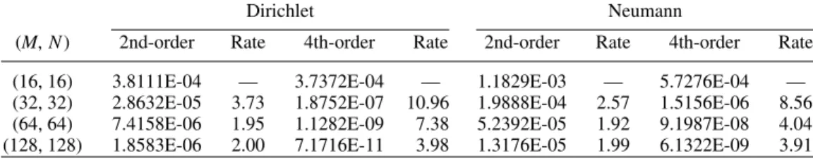
This example was first designed in [6] for the problem inside the ellipse centered at (0, 0) with major and minor axes of 2 and 1. The authors used this problem as a test of their collocation scheme for Poisson equation on a curved domain. (They did not solve the problem in the elliptical coordinates.) An interesting property is that the solution is symmetric for all four quadrants. The relative errors for the second- and fourth-order methods and their rates of convergence can be found in Table I. One can see that the magnitude of the error for the fourth-order scheme is significantly smaller than the error for the second-order scheme when the number of grid points M and N are greater than 32. Besides, the ratios for second- and fourth-order methods approach 2 and 4, respectively. This indicates that our schemes are convergent as the rates we expect for both Dirichlet and Neumann problems.
Example 2. The second solution [7] of the problem is
u共x, y兲 ⫽ x3
ex共y ⫹ 1兲cos共x ⫹ y3兲.
(4.3)
TABLE II. The numerical results obtained by the second-order and compact fourth-order Poisson solvers in an ellipse for Example 2.
(M, N )
Dirichlet Neumann
2nd-order Rate 4th-order Rate 2nd-order Rate 4th-order Rate (16, 16) 7.4693E-04 — 7.3726E-04 — 2.0005E-03 — 9.8690E-04 — (32, 32) 1.8849E-05 5.31 2.3627E-08 14.93 2.8634E-04 2.80 3.5194E-06 8.13 (64, 64) 4.8655E-06 1.95 1.5113E-09 3.97 7.2724E-05 1.98 2.4390E-07 3.85 (128, 128) 1.2212E-06 1.99 9.5420E-11 3.99 1.8371E-05 1.99 1.6045E-08 3.93 TABLE I. The numerical results obtained by the second-order and compact fourth-order Poisson solvers in an ellipse for Example 1.
(M, N )
Dirichlet Neumann
2nd-order Rate 4th-order Rate 2nd-order Rate 4th-order Rate (16, 16) 3.8111E-04 — 3.7372E-04 — 1.1829E-03 — 5.7276E-04 — (32, 32) 2.8632E-05 3.73 1.8752E-07 10.96 1.9888E-04 2.57 1.5156E-06 8.56 (64, 64) 7.4158E-06 1.95 1.1282E-09 7.38 5.2392E-05 1.92 9.1987E-08 4.04 (128, 128) 1.8583E-06 2.00 7.1716E-11 3.98 1.3176E-05 1.99 6.1322E-09 3.91
In contrast to Example 1, the solution now has no symmetry. Table II shows the relative errors and the rates of convergence for different number of grid points M and N. Again, the desired accuracy of our methods for both Dirichlet and Neumann problems has been achieved.
Example 3. The last example is given by
u共x, y兲 ⫽ 共共x ⫹␣兲5/2⫺ 共x ⫹␣兲兲共y ⫹ 兲5/2⫹ 共共x ⫹␣兲 ⫺ 共x ⫹ ␣兲5/2兲共y ⫹兲,
(4.4)
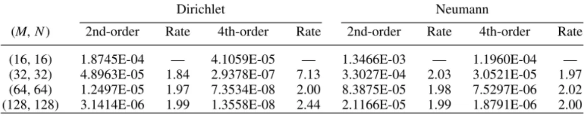
where␣ ⫽ a cosh b and  ⫽ a sinh b. Notice that, the solution has a discontinuity in the “2.5” derivative. This non-smooth property causes the rate of convergence to be at most second-order. However, one can see the errors of fourth-order scheme are again smaller than the ones obtained by the second-order scheme, see Table III in detail.
V. CONCLUSIONS
We present a simple and efficient fast direct solver for the Poisson equation inside a 2D ellipse. We first formulate the equation using the elliptical coordinates and then use the truncated Fourier series expansion to derive a set of ordinary differential equations. Those Fourier mode equations are then solved by finite difference discretizations. Using a grid by shifting half mesh away from the pole and incorporating the symmetry constraint of Fourier coefficients, the numerical boundary value near the coordinate singularity can be easily derived. Both second- and fourth-order accurate schemes for Dirichlet and Neumann problems are presented. In particular, the fourth-order scheme belongs to a compact type. The total computational cost of the method is O(MN log2N ) arithmetic operations for M ⫻
N grid points.
The author thanks the Department of Mathematics in HKUST for their hospitality during his visit where this work was initiated.
References
1. W. E and X.-P. Wang, Numerical methods for the Landau-Lifshitz equation, SIAM J Sci Comp 38 (2000), 1647–1665.
2. C. J. Garcı´a-Cervera, Z. Gimbutas, and W. E, Accurate numerical methods for micromagnetics simulations with general geometries, J Comput Phys 184 (2003), 37–52.
3. M.-C. Lai and W.-C. Wang, Fast direct solvers for Poisson equation on 2D polar and spherical geometries, Numer Methods Partial Differential Eq 18 (2002), 56 – 68.
TABLE III. The numerical results obtained by the second-order and compact fourth-order Poisson solvers in an ellipse for Example 3.
(M, N )
Dirichlet Neumann
2nd-order Rate 4th-order Rate 2nd-order Rate 4th-order Rate (16, 16) 1.8745E-04 — 4.1059E-05 — 1.3466E-03 — 1.1960E-04 — (32, 32) 4.8963E-05 1.84 2.9378E-07 7.13 3.3027E-04 2.03 3.0521E-05 1.97 (64, 64) 1.2497E-05 1.97 7.3534E-08 2.00 8.3875E-05 1.98 7.5297E-06 2.02 (128, 128) 3.1414E-06 1.99 1.3558E-08 2.44 2.1166E-05 1.99 1.8791E-06 2.00
4. J. C. Strikwerda, Finite difference schemes and partial differential equations, Wadsworth & Brooks/ Cole, 1989, p 68.
5. B. Fornberg, A practical guide to pseudospectral methods, Cambridge University Press, 1996, p 17. 6. E. Houstis, R. Lynch, and J. Rice, Evaluation of numerical methods for elliptic partial differential
equations, J Comput Phys 27 (1978), 323.
7. L. Borges and P. Daripa, A fast parallel algorithm for the Poisson equation on a disk, J Comput Phys 169 (2001), 151–192.