A FINITE-DIFFERENCE METHOD FOR SYMMETRICAL POSITIVE DIFFERENTIAL-EQUATIONS

JANUARY 1994, PAGES 105-118

A FINITE DIFFERENCE METHOD

FOR SYMMETRIC POSITIVE DIFFERENTIAL EQUATIONS

JINN-LIANG LIU

Abstract. A finite difference method is developed for solving symmetric pos-itive differential equations in the sense of Friedrichs. The method is applicable to partial differential equations of mixed type with more general boundary con-ditions. The method is shown to have a convergence rate of 0(hxl2), h being the size of mesh grid. Some numerical results are presented for a model problem of forward-backward heat equations.

1. Introduction

In the theory of partial differential equations there is a fundamental dis-tinction between those of elliptic, hyperbolic, and parabolic types. Friedrichs [5] developed a theory of symmetric positive linear differential equations in-dependent of type. The theory of Friedrichs's systems has been shown to be very useful in theoretical analysis for mixed-type problems such as the Tricomi problem and forward-backward heat equations. Furthermore, it also gives a simple and unified numerical treatment for these problems (see e.g. [1, 7, 9]). Otherwise, if a numerical method applies directly to a PDE of mixed type, the treatment of the interface on which the PDE changes type is in general very

diffi-cult to handle. For example, Vanaja and Kellogg [12] used an iterative method

to solve discrete approximations of a forward-backward heat equation which involve three different systems, i.e., forward, backward, and interface finite

dif-ference systems. The method requires the solution of the equation to be more

regular than that of the unified method proposed here. The unified method, on the other hand, not only requires less regularity for the solution but also applies to a more general setting of the problem; by this we mean less restriction on the assumption of coefficient functions that cause the equation to change type.

Several numerical methods have been developed for Friedrichs's systems [7, 9, 10]. Friedrichs [5] was the first to propose a finite difference procedure for the numerical solutions of symmetric positive systems in rectangular regions. Chu [4] further studied this method and extended it to curvilinear rectangular domains, but the rate of convergence was not established. Katsanis [7] gave a finite difference method for the Tricomi problem, using symmetric positive systems, which is applicable to any region with piecewise smooth boundaries,

Received by the editor April 16, 1992 and, in revised form, November 24, 1992 and February 16, 1993.

1991 Mathematics Subject Classification. Primary 65N30, 35K20.

Key words and phrases. Finite difference method, Friedrichs's positive systems, error estimates. This work was supported in part by NSC-grant 81-0208-M-009-513, Taiwan, R.O.C.

© 1994 American Mathematical Society

0025-5718/94 $1.00+ $.25 perpage

and showed that the rate of convergence is 0(hx/1), where h is the size of a regular mesh. However, he imposed on the system an extra constraint that the boundary matrix should be positive definite. This appears to be somewhat restrictive for the application of Friedrichs's theory. In fact, this work is mo-tivated by forward-backward heat equations which do not reduce to symmetric positive systems having this property, and we find that the constraint is actually not required for our method. We show that for a rectangular domain the rate of convergence is also 0(hxl2). The main difference between our method and the method of Katsanis is that the approximation in Katsanis's scheme does not necessarily go beyond the boundary, whereas our method does. The bound-ary condition of the system is handled differently as well. It is shown in [4] that there exists a transformation of the dependent variables, coefficient

matri-ces, the differential equations, and the boundary conditions such that when the

domain is mapped from a curvilinear rectangle to a rectangle, the symmetric positive character of the equation is preserved. We confine our considerations to rectangular domains.

Since the development of the proposed method is primarily motivated by forward-backward heat equations, we stress further the main results of both the iterative method in [ 12] and our method. For problems in the x-y plane, if the solution has continuous derivatives of order 4 in x and order 2 in y, the rate of convergence of the discretization error for the iterative method is 0(h2 + k), where h and k are mesh sizes in x and y, respectively. The iterative process may be affected by different h and k and hence by the interface system. Our method instead requires the solution to have smoothness of order 3 in x and 2 in y, and gives an 0(hx/2) convergence. Since the solution is obtained by reducing the original second-order equation into a first-order system, it is

essen-tially equivalent to a convergence rate of 0(h3/2), at least in the x-direction if

the original equation were solved directly for the unknown function.

2. Symmetric positive systems

Let Q. be a bounded open set in Rm , with a piecewise continuously differen-tiable boundary 9Í2. A point in Rm is denoted by x — (Xi, x2,... , xm) and an unknown r-dimensional vector-valued function defined on Q is given by u = («i, «2, ... , ur). Let ax, a2, ... , am be symmetric r x r matrix-valued functions, G an rxr matrix-valued function, and i= (f\, f2, ... , fr) a given r-dimensional vector-valued function, all defined on Í2. It is assumed that the a' are piecewise differentiable. For convenience, let a = (a1, a2, ... , am), so that we can use expressions such as

v ■(«) =

£^(a'u)-,=1 ax'

With this notation we can write the identity

m Q m Q /

1 1=1 (=1

simply as

A symmetric system of linear differential equations with boundary conditions can then be written in the following generic form:

(2.2) Ku := a • Vu + V • (au) + Gu = f(x) inQ,

(2.3)

Mu:=(p(x)-ß(x))u(x)

= 0 on 9fi.

The matrix ß is defined (almost everywhere) on <9fi by ß = n • a, where n = («i, ... , nm) is the outer normal on du.. The matrix p is defined on du. so that the boundary condition (2.3) is admissible and the operator K is positive in the sense of Friedrichs [5], i.e.,

(i) j(/í(x) + p*(x)) is positive semidefinite on dCl, (ii) ker(p - ß) e ker(/z + ß) = W on 30., and (iii) ^(G + G*) is positive definite in Q..

The adjoint operators K* and M* of K and M, respectively, are formally

defined by

K*\ = -a • Vv - V • (av) + G*v,

M*v = {/i* + ß)\.

Let (u, v) = Jau -\dx, and (u, v) = JdQu • ví/s. Let Hm(Q), m > 0, be

the usual, in vector form, Hubert spaces equipped with the norm || • \\m . The

following results are given in [5]:

Lemma 2.1 (First Identity). If K is symmetric positive, then for any u, v e HX(Q),

(2.4) (Ku, v) + {Ma, v) = (u, iTv) + (u, M*v).

Lemma 2.2 (Second Identity). If K is symmetric positive, then for any u G

Hx(Çl),

(2.5) [Ku, u) + (Mm, u) = (Gu, u) + (pu, u).

Let V = Cx(Çl) n {v : M*v = 0 on dfi}. We shall say that u 6 L2(Çi) is a

weak solution of problem (2.2), if for all v e V

(u,K*y) = (t,y).

The existence of weak solutions of (2.2), (2.3) is guaranteed if M is semi-admissible. Uniqueness is insured if we look for solutions in HX(Q.). If, in addition, M is admissible and a weak solution is continuously differentiable, then it must also be a classical solution. It follows from the First Identity (2.4) that a classical solution is also a weak solution [5].

3. Finite difference method

We describe a finite difference approximation of (2.2) and (2.3) for a rect-angular domain in the x-y plane. Extension to rectrect-angular domains in higher

dimensions is immediate. Let Q. be the rectangle centered at the origin, with

boundaries x = x_ , x = x+ , y = y_ , and y = y+ . Let Q be partitioned in a square grid of width h ; a grid point is denoted by a pair of integers (/, j)

with (-1 - 2, -J - 2) < (i, j) < (I + 2, J + 2) ; the step h is selected so that

boundary points (including the four corner points); those with / < |z'| < / + 2

or J <\j\< J + 2 are extensions of the domain beyond the boundary and shall be called extension points.

We introduce the shift operators

Sxu(i, j) = u(i+\, j), S»u(i,j) = u(i,j + 1), S~xu(t, j) = u(i - 1, ;)', S~yu(i, j) = u(i, j - 1).

We have S2x = SXSX , S~2x = S~XS~X and similarly for S2y and S~2y . The boundary operators 5° and Bx are defined such that B°u is the value of u on the boundary and Bxu is the value of u one row beyond (into extension) the boundary. The operator B~x is defined so that B~xu is the value one row within (into interior) the boundary, and B2, B~2 etc. are similarly defined. (E.g. Bx = SXB° at x = x+ , Bx = S~XB° at x = X- , etc.)

For each interior and boundary point, we define the finite difference operator Kn , an approximation to the differential operator K :

(Sxax)S2xu-{S-xax)S~2xu {Sya2)S2yu - (S~ya2)S-2yu „

KhU

=-Th-+-5-+

Gu-The difference equation is written for each even interior point and boundary point:

(3.1) Khu = f.

To each boundary point, we assign the approximate boundary condition (3.2) Mhu = (Bxp)B°u - (Bxß)B2u = 0,

where Bxß is defined as nxBxax + nyBxa2 at each row grid Bx, nx and ny

being well defined for each boundary. Note that, at the corner points, nx and

ny are not unique but will be well defined if we consider that (3.2) is computed piecewise on the boundary, i.e., piece by piece parallel to row Bx . In fact, this will give a unique representation of each unknown into the extension in terms of the unknown on the boundary including the four corner points. We define Bxp as

(3.3) Bxp = Bxß + M.

Clearly, the difference equation and the approximate boundary condition indeed approximate the differential equation and the given boundary condition; i.e., if u(x, y) is a continuously differentiable function defined in the closed rectangle, we see immediately that Knu converges pointwise to A^u, and Mnu converges pointwise to Mu, as h tends to 0. The values of the function at the boundary, and even in the extension, are all solved for as unknowns. This differs from usual finite difference procedures for boundary value problems, where the values on the boundary are known data. The finite difference method of Katsanis [7] is based on the formulation obtained by applying Green's theorem in any region in Q centered at each grid point. We shall see there exists a unique solution of

(3.1), (3.2).

We define the inner product and the norm respectively by (u, v)h = ^u-v4hJ

where VJe indicates summation over all even points (i,j) with \i\ < I, \j\ < J, and \\u\\n + (u, u)lJ . These can be interpreted as ordinary Hubert space inner product and norm, if the values of u defined at even grid points are interpreted as values of piecewise constant step functions, constant in each 2h x 2h square centered around each grid point. Let L2h(Q.) denote the space of these discrete functions.

Similarly, we define (u, \)n = Y,b u' y^h , where YJB indicates summation over all even boundary points with |/'| = / or \j\ = J, and \u\n = (u, u)^' . The interpretation is completely similar.

From the definitions of || • \\n and | • \n, we have the inequality

(3.4)

M, < -L/r^iiuH,.

Now, we define the consistent finite difference operator and approximate

boundary operator for the adjoint operators K* and M*, respectively:

(Sxax)S2xv - (S-xax)S~2xv (Sya2)S2yv - (S-ya2)S-2yy _,

K"v =-Th-Th-+

Gy'

M*hv = (Bxp)*B°y+(Bxß)B2y.

Let H¡ be the set of all even interior grid points in Q, and Hß the set of all even boundary grid points in dQ.. Let H = H¡\jHb . With each grid point Xj e H we identify a 2/z x 2/z mesh region P¡. If P¡ is adjacent to i\ we say that x¡ is connected to x¿ . Now define Aj to be the area of P¡, which is 4/z2, and Lj^ to be the length of the line segment between Pj and P^ . We denote Tj^ = P¡ n P^ . We use the notation YLk t0 mdicate a sum over points, xk , which are connected to some point, Xj .

We now show the discrete version of (2.4).

Lemma 3.1 (First Discrete Identity). // v and u are functions defined at even grid points, then

(3.5) (Khu, v)h + (Mnu,y)n = (u, K¡y)n + (u, M*hv)h.

Proof. At each grid point x¡ € H, we write

1 k

:= ~((Sxax)S2xu - (S-xax)S~2xu + {Sya2)S2yu - (S-ya2)S~2yu),

where u^ = u(x^), and y¡ ^ denote, in order, the values of a1, -a1, a2, and -a2 at the centers of Yjk which correspond to the east, west, north, and south

sides of Xj, respectively. Note that if r, k is beyond the boundary, we have

7j,k = ßj,k ■ Hence, at Xj e H,

Aj(Khu)j = Y,Lj,kïj,kUk + AjGuj.

k

Similarly,

We then have

(Ai«, »)„-(«,-JtMt

-E

E Lj,k(yj,k»k • ▼/ + JV.ifcT* • Uy) + ¿y(Glly • Vy - G*Vy • Uy) Since yy i- = -7k,j, and since a1 and a2 are symmetric, we have, by rear-rangement,

E E Lj.kyj,k"k

•u; = - E E lj.w • yj,k*k,

j k j k

and we see that all terms cancel with the exception of the boundary terms.

Therefore,

(3.6) (tfAn,v)A-(u,jrçv)A = £

_{E LJ Mßj, kuk * Vy}

_{+ ßj, fcV*}

_{• Uy)}

_k£I

On the other hand, at each xy e i/ß, we have

(Mhu)j = (Bxß + p- ß)j(B0u)j - (Bxß)](B2u)]

= (ßj,k+ßj- ßj)"j- ßj,kUk,

and

(M*hy)j = (Bxß + p- ß))(BQv)j + (Bxß)](B2y)]

= (ßlk+p*-ß*j)yj

+ ßjtkyk,

where k g I. Hence,

(u, M¿y)h - (Mnu, y)h = ^

jen

YsLJ,k{ßi,k*k' vy + ßj,k"k ■ vy) which is the same as the right side of (3.6). Hence (3.5) is proved. D

Observe that Kh+K* = G + G* and Mh + M£ = (Bxp) + (Bxp)* . By setting v = u in (3.5), we get immediately the discrete version of (2.5).

Lemma 3.2 (Second Discrete Identity). For functions u defined at even grid

points, there holds

(3.7) (Khu, u)h + (Mhu, u), = (Gu, u)A + ((Bxp)u, u)h. Consequently, we have:

Lemma 3.3 (Basic Inequality). For u satisfying the approximate boundary con-dition Mhu = 0, there is a (generic) constant C > 0 such that

\\u\\h < C\\Khu\\h.

The existence and uniqueness of the solution of (3.1), (3.2) can be proved as follows. We see that the unknowns in (3.1) include those at the boundary and in the extension. For unknowns in the extension, we substitute the boundary

condition (3.2) into (3.1). Note that

Bxß = Sxax, B2u = S2xu onx+,

etc. Hence, by substituting

(Bxß)B2u = (B''p)B°u

into (3.1 ), we then have a square finite system of linear equations with unknowns at all grid points x¡ e H (not including the points in the extension). The Basic Inequality insures uniqueness of the solution of the system of linear equations. But since these equations are a square finite system, uniqueness of the solution also insures its existence. We summarize:

Theorem 3.1. The system of finite difference equations (3.1) and boundary

con-dition (3.2) possesses a unique solution.

We now study the error between the approximate solution u/¡ of (3.1), (3.2)

and the solution u of (2.2), (2.3).

We may express K in a form slightly different from (2.2), by the use of (2.1).

That is,

(3.8) Ku = 2V • (au) - (V • a)n + Gu.

In order to relate L\(Çï) to the usual L2(fi) space, we introduce a projection

rh: C°(U) ^L2(ÇÏ) defined by

(rhu)j = u(Xj), Vx;G/7,

and an injection p„: Lj(Çl) —> L2(Q) defined by

phuh(x) = (uh)j, VxeP/nil

We immediately have ||pauaIIo < I!uaIIa ' ^Vfi e ^a(^) •

We shall need the following lemma which is given in [7].

Lemma 3.4. Let g be a function defined on a finite region P c R2, and suppose that g satisfies a Lipschitz condition, i.e., there is a constant C > 0 such that

\g(x) - g(y)\ < C\x - y\ for all x, y e P. Then, if A is the area of P and

|x - xo| < h in P, we have

g(x0) -¿I

S(x) < Ch.

We now state the convergence properties of the method.

Theorem 3.2. Suppose that u G C2(Q) is the solution of (2.2), (2.3). Let u„ G L2h(Çl) be the unique solution of (3.1), (3.2). Then

(3.9) \\rhKu-Khrhu\\h = 0(h),

(3.10) \rhMu-Mhrhu\h = 0(h).

Moreover, the discrete error converges at the rate (3.11) \\uh-rhu\\h = 0(hi'2), (3.12) ||^uÂ-u||o = 0(/ï1/2).

Proof. Using the Second Discrete Identity (3.7), the positive definiteness of G and positive semidefiniteness of p , we have for some constant C > 0

Writing Kf,(un - rnu) = rnf-rnf+ rnKu- K„rnu, using the boundary conditions

^aua = ff,Mu = 0 on Hg and the Cauchy-Schwarz inequality, we have

l|uA - rhu\\2n < C[\\u„ - rhu\\h\\Kh(uh - rhu)\\h + \u„ - rhu\h\Mh(uh - rhu)\h] = C[\\u„ - r„u\\h\\rhKu - Khrhu\\h + \uh - rhu\h\Mhrhu\h\.

We shall show that \\rhKu - Khrhu\\h = 0(hx) and \Mhrhu\„ = 0(hx). Then,

(3.4), (3.9), and (3.10) imply (3.11).

From the definition of || • ||/2, we have

\\rhKu - Khrhu\\2h = $>** « - Khrhu)24h2.

e

We now obtain a suitable bound for |A^u(x;) - (Knrhu)j\. By (3.8), \Ku(Xj) - (Khrhu)j\

1

(3.13)

_<

2V • (au)(Xj) - (V • a)u(Xy) - -j- V-Ly^y,*»*

Aj k

2V • (au)(Xj) - ir E LJ,k7j,k{Ok + uy)

Aj

+

(V-a)u(xJ)---Y,LJ,kyj,kUj

Consider the first term in the last expression above: 1 v^

2V • (au)(Xj) - ■j-2^Lj,kyj,k(Uk + Uj, Ai 1. <

(3.14)

2V • (au)(xy) - j- [ V-(au) Ai JPj + + 1

Aj

W

2(yu-(yu)j>k)

k 7r^ E / (2(>'u)j,fc-7y,Ä(Ufc+u;))

Using Lemma 3.4, we have

(3.15)

2V • (au)(x

*-hk-

(au)

= 0(h).

We now examine a Taylor series expansion for yu about the point Xy* =

(xy+Xjt)/2:

(3.16) y(xJik + tz)u(Xj,k + tz) = (yu)j,k + t(j-((yu)j + y#(¿;1),

where z is a unit vector orthogonal to Xj-xk , t is a scalar parameter, g(Ç) =

(¿?i(<Üi)> glib))> gi is the /th component of the vector (d2/dt2)(yu), and &

is a point on the straight line between x]k + (Ljk/2)z and x¡k - (Ljk¡2)z .

Using (3.16) and (3.17), we obtain the following bound:

(3.18) / yu-(yu)Jtk = O(h').

Since u G C2, we have

h2 h2

Uj = ujik - hu'j k + yu"(íi), uk = ny,* + hu'jk + yu"fe),

where the derivatives are directional derivatives in the direction xk—x¡. Hence, we have

|2uy,* -(uy + u*)| < Ch2. This means that

/ yj,k(2uj

Jr¡,k k-(Uj + Uk))

(3.19)

<Lj,k\\yj,k\\\2uJ,k-(uJ+uk)\ = 0(h3).

Using (3.15), (3.18), and (3.19) in (3.14), we obtain

(3.20)

2V-(au)(xy)-^£Ly>jtyyi*(ujt

+ uy) =0(h).

AJ k

We now consider the second term on the right of (3.13):

1

(V • a)u(xj) - —JTLj^yj^Uj

(3.21)

<

(V • a)u(xy) - -j- / (V • a)u Ai JPj - /(V-a)(u-Uy) + -j-]T / (7-7j,k)*j j JPj jkJri-k

Again, by Lemma 3.4, we get

(3.22)

(V-a)u(xy)-^- /(V-a)u

Aj JPj

0(h).

Since u satisfies a Lipschitz condition, |x - Xy| < h for all x G P¡, and since || V • a||o is uniformly bounded in Q,, we have

(3.23)

J-^(V.a)(u-«y;

< ||V-a||o|u-Uy| = 0(h).

Since 7jk is evaluated at the midpoint of r; k, we can use a Taylor series

analysis, as in deriving equation (3.18), to get

Combining (3.22), (3.23), and (3.24) in (3.21), we obtain

(3.25)

(V • a)u(xf

}E%

kVj.kUj

= 0(h).

Substituting (3.20) and (3.25) in (3.13), we obtain

\Ku(Xj)-(Khrhu)j\ = 0(h),

from which (3.9) follows. Next, we prove (3.10). By (3.3), we have Mnrhu = BxpB°rhu - BxßB2rhu

= BxpB°rhu - MB°rhu - BxßB2rnu = BxßB°rhu-BxßB2rhu.

Hence,

\Mnrnu\n<\Bxß\h\B0rnu-B2rhu\h

^EE / ■■

U/t

for all Xy G HB, which implies that \Mhrhu\n = 0(h), i.e., that (3.10) holds. Finally, we prove (3.12). We have

IIPaUa

- «Ho

= II/Va" - Pa^a" - oa) - o||o

< Hpa^u - u||o + \\ph(uh - rhu)\\0.

Since and

WPhiuf, - rhu)\\o < ||uA - rÄu||A,

||/7„r„u-u||2 = W (uj-u)2 = 0(h2),

, Jo,'Qj

where Qj = Pj n Q., we get (3.12). This concludes the proof. D

Remark. In the proof of this theorem, we did not require p + p* to be strictly positive definite; Katsanis [7] proved the rate of convergence using this con-dition. The domain considered in this paper is a rectangle, and the rate of convergence we have achieved is 0(hxl2). If a more complicated domain is encountered with piecewise smooth boundary, then Katsanis's finite difference

scheme can be used. In this case the rate of convergence would still be 0(hxl2) ; however \\rhKu - Khrhu\\h would be 0(hx/2) instead of 0(h). Note that (3.9)

and (3.10) can be interpreted as the consistency of the operators K and Kh and the operators M and Mn, respectively.

4. A MODEL PROBLEM

Katsanis's method was motivated primarily by the numerical treatment of the Tricomi problem, which reduces to a first-order system with positive definite boundary matrix p in (2.3). The following model problem shows that the above restriction needs to be removed and hence the method given in the previous section can be used. We consider the boundary value problem

f-0(±l,y) = O, VyG[0,l],

(4.2)

Ï 0(x,O) = O, Vxg[0, 1],

U(x,l)

= 0, Vxg[-1,0],

where Q. = (-1, 1) x (0, 1) and the coefficient o(x, y) changes sign in Q.. There have been a number of papers addressing this kind of mixed-type heat equations (see e.g. [2, 3, 8, 11]). For a discussion of possible applications of such equations, we refer to [12].

We briefly show how the boundary value problem (4.1), (4.2) can be

formu-lated as a Friedrichs's system. By a change of dependent variables, UA, ux=e-ky<¡>, u2 = e-Xy<t>x,

equation (4.1) may be written as the symmetric first-order system

(4.3) /*iUx-M2u>,-Mou = f,

where

^ = (-°i "o1)' Al={o

o)' A°=(Xo i)' t=(eof

Note that (4.3) in general is not positive. To make (4.3) symmetric positive, we

multiply both sides by a 2x2 matrix

T _ ( a bo

Vo a

where a and b are functions of x and y to be specified later. Then the forward-backward heat equation (4.1), (4.2) can be expressed in symmetric positive form, with properly chosen a, b, and X, by

(4.4) Ku = l infi,

(4.5) Mu = (p-ß)u = 0, V(x,y)GôQ,

where

Ku = axux + (a'u)* + a2uv + (a2u)v + Gu,

i 1 (-bo -a\ 2 1 ( ao 0

a =2\-a 0 ) ' Q=2(0 0

o (Xao bo\ , (ae~kyf

01 ={ 0 a)> i=[ 0 "

G = a°-(ax)x-(a2)y, ß=U^ny-bnx)o -an, 1 ( q+ + q~ -anx

2 V -anx ß 2 \ anx 0

Here, q± are nonnegative functions defined by (anv-bnx)o = q+ -q . Then

G + G* __ 1 i2Xao - (ao)y + (ba)x bo + ax

2 ~ 2 V bo + ax 2a

will be positive definite and p will be positive semidefinite, and ker(/z - /?) ker(,u + ß) = R2.

We summarize the conditions on the choice of a, b , and X in order to have a positive system with admissible boundary condition:

(I) T is piecewise differentiable,

(II) q± are nonnegative functions on dQ.,

(III) G + G* is positive definite.

The existence and uniqueness of the solution of (4.1), (4.2) follows imme-diately by using Friedrichs's results [5]. The reduction of the second-order problem to a first-order system not only simplifies the proof of existence and uniqueness but also is more convenient for the numerical treatment of the prob-lem. Note also that, by Theorem 3.2, the solution of (4.1), (4.2) is required to have continuous derivatives of order 3 in x, compared with order 4 for the

method in [12].

We give some examples on the choice of a, b , and X.

Example 1. The case of o(x, y) = xm with m an odd positive integer has

been considered in [6]. For this we choose X = 0, a = 1, and b such that

bxm = x . After a simple calculation, we have

G + G*=(x 2)'

which is positive definite for all x G [-1, 1].

Example 2. We now show an example for which o(x ,y) = x+\y. Let X = 0.1, a = 2, and b = 1 . After a simple calculation, we have

G + G*=(* + °-2{X + i*y) X + i*y]

V x + ¡y

4 ) '

which is again positive definite for all x G [-1, 1], y G [0, 1]. As mentioned

in the introduction, the iterative method proposed in [12] requires a more re-strictive condition on the coefficient function o , namely oy < 0 in Q . Example 3. Our numerical experiment was based on the example for which o(x, y) = x. This kind of coefficient function appearing in the equation has been considered by many authors (see for example [11, 3]). In our computations / is taken to be

f(x,y) = 2x(x2 - l)y[(y -I)2- 4x2+y(y - 1)]

-2y2[(y- l)2-24x2 + 4] Vx>0, yG[0, 1],

f(x, y) = 2x(x2 - \)(y - l)(2y2 - y - 4x2)

- 2(y - l)2(y2 - 24x2 + 4) Vx < 0, y G [0, 1].

Denote the boundary dQ. by Ti U • ■ • U T6,

r, = {(x,y):xG[-l,0],

y = 0},

r2 = {(x,y):x = -l, yG[0, 1]}, r3 = {(x,y):xG[-l,0], y=l}, r4 = {(x,y):xG[0, 1], y=l},

r5 = {(x,y):x=l,

ye[0, 1]},

r6 = {(x,y):xG[0, 1], y = 0}.

To formulate (4.1), (4.2) as a symmetric positive system, we choose X = 0.1, a = 1, and b = 1. Then

,'O.lx + i x

0

1

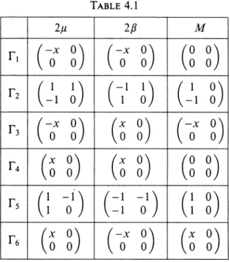
We see that (G+G*) is positive definite in Q. We need to evaluate the matrices p and ß along all boundaries. A straightforward calculation gives the values

for p, ß , and M shown in Table 4.1. Table 4.1

2p

-x 0

0 0

1 1

-1 0

-x 0

0 0

x 0

0 0

1 -1

1 0

x 0

0 0

2ß

-x 0

0 0

-1 1

1 0 x 0

0 0

x 0

0 0

-1

0

-x 0

0 0

M

0 0

0 o

1 o

-1 o

-x 0

0 o

o o

o o

1 o

1 o

x 0

o o

Of course, p is positive semidefinite. Also, ker(jU - ß) © ker(p + ß) = R2, so that the boundary condition (4.2) is admissible. Theorem 3.2 assures us of essentially 0(hxl2) convergence in the L2 norm. However, the results shown

in Table 4.2 are better, i.e., 0(h).

Table 4.2

1/4

1/8

1/12

1/16

1/20

error

14.120

6.077

4.033

3.464

3.145

L2 error

4.897

1.706

1.048

0.764

0.602

L2 rate

1.52

1.20

1.10

1.06

1/24

2.956

0.496

1.05

Acknowledgment

The author would like to thank Professor A. K. Aziz for his guidance in this work. The author would also like to express his gratitude to the referee for valuable comments on the paper.

Bibliography

1. A. K. Aziz and J.-L. Liu, A weighted least squares method for the backward-forward heat equation, SUM J. Numer. Anal. 28 (1991), 156-167.

2. M. S Baouendi and P. Grisvard, Sur une équation d'évolution changeant de type, J. Funct. Anal. 2(1968), 352-367.

3. R. Beals, On an equation of mixed type from electron scattering theory, J. Math. Anal. Appl. 58(1977), 32-45.

4. C. K. Chu, Type-insensitive finite difference schemes, Ph.D. Thesis, New York University, 1958.

5. K. O. Friedrichs, Symmetric positive differential equations, Comm. Pure Appl. Math. 11 (1958), 333-418.

6. J. A. Goldstein and T. Mazumdar, A heat equation in which the diffusion coefficient changes sign, J. Math. Anal. Appl. 103 (1984), 533-564.

7. T. Katsanis, Numerical solution of symmetric positive differential equations, Math. Comp. 22(1968), 763-783.

8. T. LaRosa, The propagation of an electron beam through the solar corona, Ph.D. Thesis, Dept. of Physics and Astronomy, University of Maryland, 1986.

9. P. Lesaint, Finite element methods for symmetric hyperbolic equations, Numer. Math. 21 (1973), 244-255.

10. P. Lesaint and P. A. Raviart, Finite element collocation methods for first order systems, Math. Comp. 33 (1979), 891-918.

11. J.-L. Lions, Quelques méthodes de résolution des problèmes aux limits non linéaires, Gauthier-Villars, Paris, 1969, pp. 337-343.

12. V. Vanaja and R. B. Kellogg, Iterative methods for a forward-backward heat equation, SIAM J. Numer. Anal. 27 (1990), 622-635.

Department of Applied Mathematics, National Chiao Tung University, Hsinchu, Taiwan