Predictive classifier for image vector quantization

Shen-Chuan Tai

National Cheng Kung University Department of Electrical Engineering Tainan, Taiwan

Yung-Gi Wu

Leader University

Department of Information Engineering

I-Sheng Kuo

National Chiao Tung Univeristy Department of Information Science

Abstract. A new scheme for a still image encoder using vector

quanti-zation (VQ) is proposed. The new method classifies the block into a suitable class and predicts both the classification type and the index information. To achieve better performance, the encoder decomposes images into smooth and edge areas by a simple method. Then, it en-codes the two kinds of region using different algorithms to promote the compression efficiency. Mean-removed VQ (MRVQ) with block sizes 8

⫻8 and 16⫻16 pixels compress the smooth areas at high compression ratios. A predictive classification VQ (CVQ) with 32 classes is applied to the edge areas to reduce the bit rate further. The proposed prediction method achieves an accuracy ratio of about 50% when applied to the prediction of 32 edge classes. Simulation demonstrates its efficiency in terms of bit rate reduction and quality preservation. When the proposed encoding scheme is applied to compress the ‘‘Lena’’ image, it achieves the bit rate of 0.219 bpp with the peak SNR (PSNR) of 30.59 dB. © 2000 Society of Photo-Optical Instrumentation Engineers. [S0091-3286(00)00908-9]

Subject terms: vector quantization; mean-removed vector quantization; predictive classification vector quantization.

Paper 990206 received May 28, 1999; revised manuscript received Jan. 18, 2000; accepted for publication Feb. 3, 2000.

1 Introduction

Image and video compression approaches have received considerable emphasis in many applications to increase the transmission or storage efficiency. These techniques have successfully applied in video phone conferencing, high-definition TV 共HDTV兲, image storage, or transmission. Vector quantization共VQ兲 has developed as one of the most efficient image coding techniques.1,2 The image to be en-coded is first processed to yield a set of vectors. A code-book is generated from a set of training vectors. The most commonly used algorithm to obtain a codebook is an itera-tive clustering algorithm such as K-means, or a generalized Lloyd clustering algorithm 共LBG兲, proposed by Linde, Buzo, and Gray.3 Each input vector is individually quan-tized to the closest codevector in the codebook. Compres-sion is then achieved using the indices or labels of the codevectors for the purpose of storage and network trans-missions. The image can be reconstructed using look-up table techniques with indices to select the corresponding codevectors from the same codebook as the encoder used. The major advantage of VQ is its simple implement on the hardware of the decoder.

There are many VQ research topics to increase the com-pression efficiency, including finite state VQ共FSVQ兲 共Ref. 4兲, address VQ 共AVQ兲 共Ref. 5兲, classification VQ 共CVQ兲 共Refs. 6 and 7兲, and predictive VQ 共PVQ兲 共Refs. 8–11兲, side-match VQ共SMVQ兲 共Ref. 12兲, and index-compression VQ共Refs. 13–15兲. The proposed method is a PVQ strat-egy. In PVQ schemes, image blocks are usually very small, typically 4⫻4, and therefore a high correlation exists among the blocks in a neighborhood. Thus, correlation can be used to predict the index of next codeword that will be encoded. The proposed method utilizes the edge orientation

to raise the correct prediction ratio. Simulation results dem-onstrate that it is an efficient and effective coding scheme because it outperforms the results of already mentioned and the Joint Photographic Experts Group共JPEG兲 compression schemes.

In the next section, we introduce VQ briefly. Section 3 presents the proposed new method, including the method-ology to classify the image into different classes and to use the prediction technique to reduce the overhead among edge regions. The simulation result are given in Sec. 4. Finally, Sec. 5 presents the conclusion and discusses our future research work.

2 Brief Reviews of VQ

The basic idea of VQ is quite simple, representing se-quences of input vectors with a much smaller set of pre-defined vectors, which are called codevectors. On the de-coder side, VQ can reconstruct the sequences, using a look-up-table method to retrieve the codevectors from the codebook, and it outputs as the reconstructed sequences.

Formally, a VQ of k dimension and size N can be re-garded as a mapping Q from a k-dimensional space Rkto a finite subset Y of Rk. That is,

Q:Rk→Y, 共1兲

where contains N reference vectors in Rk or is called the codebook, yi represents the i’th codevector in Y, and N

stands for the codebook size. When fixed-length binary codes are used to label the codevectors in codebook Y and each code length is fixed at l bits, the size of codebook

should be limited to N⫽2l. In fact, the mapping Q can be expanded into the composition of two mappings, encoder E and the decoder D, i.e.,

Q共x兲⫽D关E共x兲兴, x苸Rk

E:Rk⫺I 共2兲

D:I→Y

where I⫽兵1, 2, . . . , 2l其is a set of codebook indices. Each index is associated to only one codevector in the codebook through the searching criteria. With these two mappings, the function of a VQ can be indirectly accomplished as follows. The VQ encoder E, which is occasionally called the vector quantizer, assigns the input vector x to an index

i as output according to one encoding rule. Subsequently,

this index i is used under the VQ decoder D on the receiver side to determine the reconstruction vector Q(x). Due to the data to represent index i is less than original input vec-tor x, the goal of compression is achieved. Detailed de-scription of VQ can be found easily from Refs. 1–3. 3 Predictive Classifier for VQ

3.1 Classification

Classification is used to recognize characters and specify an image block to a suitable class. It is often used to segment an image into small blocks first before applying a compres-sion algorithm to increase efficiency. There are many dif-ferent methods to classify image blocks. In this paper, a new method by gradient is used to classify image blocks. The main goal is to classify the block into edge and smooth classes, which can be employed with different compression schemes to raise efficiency.

For a 4⫻4 block B⫽兵Xi j;0⭐i, j⭐3其 to be classified,

where Xi j is gray level of the pixel corresponding to

posi-tion 共i,j兲. First, find the maximum Xmax and the minimum

Xmin in block. If the difference between Xmax and Xmin is smaller than a threshold t, the block is classified as a shade block; otherwise, it will be classified as an edge block. In most conditions, the gray-level difference between two sides to form an edge is about 25 to 30. According to this and experimental visual testing, 20 to 30 is a reasonable value of t.

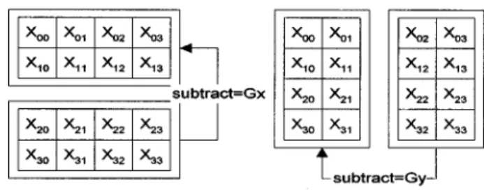
Once a block is classified as an edge block, the orienta-tion of edge pattern within block will be computed as an aid to classification. First we compute the gradient both in x and in y directions. Gx⫽

兺

兺

兺

兺

兺

兺

兺

兺

For more clarity, the computation of Gx and Gy is

illus-trated as Fig. 1.

Once the G_x and G_y are computed, we compute the orientation of block by

D⫽tan⫺1

冉

冊

. 共4兲

Then, dividing the orientation into four groups: ⫹0, ⫾90, ⫹45, and ⫺45 deg. Each group contains the range of 45 deg. Therefore, group of ⫹0 deg corresponds to edge blocks of⫺22.5 to ⫹22.5 deg. The detailed relationship list of groups, degrees, and classification types are presented in Table 1.

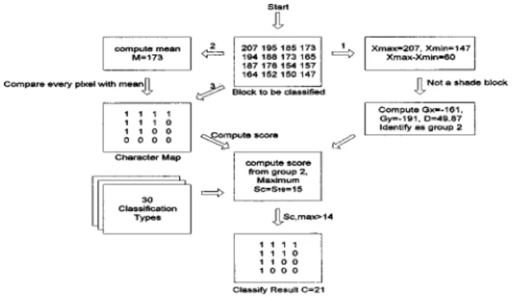
In the last step, the exact classification result is decided. We compute the mean of the block as follows:

M⫽ 1 16i

兺

兺

Then a character map is built according to the mean value. If the gray level of a pixel is greater than or equal to M, we assign a 1 to the corresponding position on the character map. Otherwise, we assign a 0 to the map. A detailed de-scription is given simply as

C Mi j⫽

再

1 Xi j⭓M

0 Xi j⬍M

, i j⫽0 to 3. 共6兲

Using the described methods, a character map of each desired block is obtained. Then, the similarity between the character map and all classification types is computed to assign it to a suitable and exact class. The classification type Tcs are shown in Fig. 2, which labels 32 classes of 4

⫻4 block. While calculating the similarity, we assume the black blocks in Fig. 2 are equal to 1, and white blocks are equal to 0. The equation below is to calculate similarity score Sc of each input X:

Fig. 1 Computation gradients in thexandydirections.

Table 1 Relationship between groups, degrees, and classification

types.

Group Degree Degree Ranges Classification Types (Tc)

0 ⫹0 ⫺22.5 to⫹22.5 1, 2, 3, 4, 5, 6, 7 1 ⫾90 ⬎⫹67.5 or⬍⫺67.5 8, 9, 10, 11, 12, 13, 14 2 ⫹45 ⫹22.5 to⫹67.5 15, 16, 17, 18, 19, 20, 21, 22 3 ⫺45 ⫺22.5 to⫺67.5 23, 24, 25, 26, 27, 28, 29, 30 Tai, Wu, and Kuo: Predictive classifier for image vector quantization

Sc⫽

兺

兺

再

Class c, which has a maximum score Sc, is returned as

classification result. If the score of classification result c is smaller than 14, a miscellaneous block 共class type 31兲 is assigned to it. An example of the proposed classification method is given in Fig. 3.

3.2 Prediction

By observing images, we can see that the edge patterns extend and accompany the orientation. Therefore, consid-ering the edge orientation in our coding scheme can pro-mote a reasonable performance.

3.2.1 Prediction on classification types

While predicting the classification types, the types of neighboring block should be considered to increase the pre-diction correct ratio. Four blocks labeled L, U, LU, and RU, respectively, as shown in Fig. 4, are considered as an aid to increase prediction efficiency. The block that needs to be predicted is marked as X. As we described in Sec. 3.1, the classification types are divided into six groups, including the four edge groups listed in Table 1 and shaded共smooth兲 and miscellaneous types. Briefly, the idea is that edges should be continuous in natural images; that is, if the left side of block X共block L兲 has a classification type of group 0共0 deg, horizontal edge兲, there is a large probability that X has the same classification type with L, as illustrated in Fig. 5.

When a block is to be predicted, the prediction algo-rithm checks the classifications of adjacent blocks first. If the block to the left side of X does not exist共i.e., it is at the leftmost position of an image兲, X is predicted as the same type as its upper block U. In the same way, we predict X as the same type as its left side block L, if upper side U does not exist. If all four neighboring blocks exist, the prediction algorithm checks the following criteria:

Fig. 2 Classification types.

1. If the classification type of L belongs to group 0, then predict X as the same type as L.

2. If the classification type of U belongs to group 1, then predict X as the same type as U.

3. If the classification type of RU belongs to group 2, then predict X as the same type as RU.

4. If the classification type of LU belongs to group 3, then predict X as the same type as LU.

5. If one or both of L and U are miscellaneous types, predict X as a miscellaneous type.

6. If none of the neighboring blocks are shade block, predict X as a miscellaneous type.

These conditions are tested sequentially. Once a condition is satisfied, the rest of conditions are ignored. If all condi-tions can not be satisfied, then the block to be predicted may not contain an edge. Therefore, X will be predicted as a shade block.

3.2.2 Prediction on VQ indices

Once the prediction of classification type returns a correct result, i.e., the prediction hit, block X should have the same classification type as one of the neighboring blocks in most cases. By observing Fig. 5, we claim that block X can be predicted from one of the adjacent blocks 共P兲 due to the edge pattern characteristics. There is a high probability that

X has the same VQ index as P. And even if the VQ index

is not the same, the codevector of the VQ index of P may be close to X.

Prediction based on VQ indices can be integrated with prediction based on classification types. If the classification type of block X is predicted from one of the neighboring blocks P, then the VQ index of block X will also be pre-dicted as the VQ index of P. This criterion can be adapted to criteria 1 to 4, as given in Sec. 3.2.1. If the classification type of block X was predicted using criteria 5 and 6, the prediction based on the VQ index will not be applied. In this case, X is predicted as a miscellaneous type, which is the most complex part in an image; X and P will be differ-ent from each other, although they are neighboring blocks. In the resting cases, X is predicted as a shade block. Once the six criteria are passed, we must have at least one block of the shade type. Blocks L, U, LU, and RU are checked. The first shade block found is assigned as P. Then the index of X is predicted as the same as P.

3.3 Encoding Process

An image can be approximately divided into smooth and complex regions. A smooth region can be compressed at a high compression ratio with little influence on the overall quality of the reconstructed image. A complex region is hard to compress, which is a challenge for all kinds of compression schemes. The majority of storage space re-quired for a compressed image is that which stores the complex region. Moreover, the quality of a reconstructed image is greatly affected by the quality of the complex region.

While an image is being fed into the proposed encoder, the image is decomposed into smooth and edge areas by a simple method that is described later. After decomposition, the image is segmented into three kinds of image blocks of sizes 4⫻4, 8⫻8, and 16⫻16 pixels. Blocks with the size of 4⫻4 pixels are treated as edge areas, and the other blocks are treated as smooth areas. Different algorithms are applied to encode each area. A flowchart of the proposed encoder is shown in Fig. 6.

3.3.1 Decomposition process

The image to be decomposed is first divided into 16⫻16 nonoverlapping blocks. Then the variance, which denotes the complexity, of each divided block is computed. If the variance is larger than a threshold, the block is further di-vided into four 8⫻8 blocks. The same test is applied to each 8⫻8 block to determine whether the 8⫻8 block is divided into 4⫻4 blocks. An example of the decomposi-tion result is shown in Fig. 7.

3.3.2 Encoding of smooth areas

After dividing the image into smooth areas and edge areas, two areas are encoded separately. Smooth areas contain two sizes of blocks, blocks of 8⫻8 pixels and blocks of 16⫻16 pixels. Each block is encoded by mean-removed VQ 共MRVQ兲. Blocks of 8⫻8 pixels are encoded by 8 ⫻8 MRVQ, and blocks of 16⫻16 pixels are encoded by 16⫻16 MRVQ. All means are quantized to 6 bits, and a standard VQ encoder with a codebook size of 32 is applied to encode the zero-mean blocks into indices.

Fig. 5 Basic idea of prediction.

Fig. 6 Flowchart of the encoder.

3.3.3 Encoding of edge areas

After they are decomposed, we find that not all blocks in the edge areas are really edge blocks. To achieve better performance, recognizing edge blocks with different orien-tation is required of our prediction algorithm. The classifi-cation method described in Sec. 3.1 is applied to distin-guish between shade blocks and edge blocks. At the same time, the prediction of classification types is also accom-plished using the prediction method described in Sec. 3.2. Then, we test whether or not the prediction is correct. Only 1 bit is used to represent the type of block if prediction succeeds. But if prediction fails, 1 bit will be the cost as a penalty. Prediction for the classification result can reduce the overhead required by the classification.

After prediction based on classification types, we must determine whether or not prediction based on indices should be applied. Prediction based on indices is not ap-plied if the prediction based on classification types failed, or if the block is predicted as a miscellaneous block. The mean square error 共MSE兲 of the predicted index and the optimal index are computed as PMSE and OMSE, respec-tively. If PMSE-OMSE is smaller than a threshold, the pdicted index is used to replace the optimal index and re-ported as a successful prediction. Otherwise the optimal index is used, which is reported as a prediction fault. An-other bit is used to denote the prediction status. From the experimental results, the threshold for PMSE-OMSE is set to 1000. The rest of the blocks, to which we applied no VQ index prediction, are encoded directly using classified VQ. 3.4 Postprocessing

MRVQ of 8⫻8 and 16⫻16 blocks is applied to encode the smooth areas. In this way, the smooth areas can be encoded into a very low bit rate with little distortion to the overall performance. However, the decoded image will have slight blocking effects in smooth areas, as Fig. 8 shows. A simple filter is applied to the smooth areas of images to improve the visual quality. Figure 9 shows the 3⫻3 filter that is applied to the smooth image areas. This filter is equivalent to the following equation:

xˆ共u,v兲⫽ 1 兺i⫽⫺1 1 _兺 j⫽⫺1 1 w共i, j兲i⫽⫺1

兺

兺

where xˆ(u,v) is the filtered pixel in position (u,v) and

represents the central pixel in Fig. 9; w(i, j) denotes the weight number of the corresponding position; and w(0,0) represents the central location, which is 4 in Fig. 9. The blocking effects can be greatly reduced after filtering, and the overall performance of the peak SNR共PSNR兲 will in-crease about 0.1 to 0.2 dB.

3.5 Bit Allocation

The space required to store the compressed image can be split to three parts: the overhead of the decomposition and the smooth and edge areas. The first part is denoted as

BD⫽N16⫻1⫹N8⫻4, 共9兲

where N16 is the number of 16⫻16 blocks and N8 is the number of 8⫻8 blocks.

In smooth areas, means and VQ indices of blocks must be stored, thus it requires

Bs⫽共N16⫹N8兲⫻共Bmean⫹Bindex兲, 共10兲

where Bmeandenotes the bits required to quantize the mean value. Means are always quantized to 6 bits in our algo-rithm, thus, Bmeanis equal to 6. The value of Bindexdepends Fig. 7 Decomposition result for ‘‘Lena.’’ Fig. 8 ‘‘Lena’’ reconstructed before filtering; 30.22 dB at 0.219 bpp.

on the size of codebook used to encode the indices for mean-removed blocks. It can be represented as

Bindex⫽log2 共smooth codebook size兲. 共11兲

For example, if codebook size is 32, the number of bits required to encode an index is 5 bits.

Predictions are employed in edge areas. A 1 is sent to the receiver if the prediction based on classification types is correct. Otherwise, a prediction fault occurs, and a 0 is sent to indicate this. The 0 is followed by the correct classifica-tion type. If predicclassifica-tion based on types is correct, then pre-diction based on VQ indices can proceed. Another bit is used to represent the prediction result based on the indices. This bit is 1 if prediction based on index hits, otherwise it is 0, and it is followed by the optimal index number oc. Here

N_PTCdenotes the number of blocks with correct prediction in classification type and NPTF denotes the number of blocks that are not correctly predicted; NPIC denotes the number of blocks with a correct prediction in VQ indices and NPIF denotes the number of blocks that are not cor-rectly predicted. Therefore, it is clear that the number of bits used to store classification information is

Btype⫽NPTC⫻1⫹NPTF⫻共1⫹5兲. 共12兲

If prediction based on indices is not applied, the number of bits used to store indices is

Bindex⫽log2共edge codebook size兲. 共13兲

If prediction on indices is applied, then

Bindex⫽NPIC⫻2⫹NPIF⫻关2⫹log2共edge codebook size兲兴

共14兲 is required. The overhead required to store the whole edge areas is

B_E⫽Btype⫹Bindex. 共15兲

The overhead required for the entire image is thus B⫽B_D ⫹BS⫹BE.

4 Simulation Results

The proposed algorithm was simulated and applied to sev-eral gray-level images for performance evaluation. The resolution of all the tested gray images was 512⫻512. Each

pixel takes 8 bits. The quality of the encoded image is evaluated by the PSNR. The PSNR is defined as

PSNR⫽10⫻log10

冉

MSE

冊

Note that the MSE for an m⫻m image is defined as

MSE⫽1 mi

兺

兺

where xi j and xˆi j denote the original reconstructed gray

levels, respectively.

In smooth areas, two codebooks, 8⫻8 and 16⫻16, were generated by the LBG algorithm. Each codebook consists of 32 codevectors. Twenty-five 512⫻512 pixel images are decomposed by a simple decomposition method to generate the smooth regions that are fed to the training sets of code-books of smooth areas.

For the edge codebook, every type of codebook in the edge areas was also generated by the LBG algorithm, i.e., 32 codebooks with a block size of 4⫻4 were generated. Each codebook except that for the shade type consists of 256 codevectors. The codebook for the shade type consists of only 128 codevectors. The same 25 images described before, are divided into nonoverlapping 4⫻4 block. These blocks are classified into 32 groups using the classification method described in Sec. 3.1. Each group of blocks is treated as a training set for the codebook for its specified block pattern.

All the test images are not included in the training set. They are ‘‘Lena,’’ ‘‘F-16,’’ ‘‘Peppers,’’ and ‘‘Tiffany.’’ Images are decomposed first using two thresholds, one for 16⫻16 blocks and one for 8⫻8 blocks. Table 2 shows the compression performance with different decomposition thresholds. From the experimental results, the 16⫻16 threshold is assigned to 200 and the 8⫻8 threshold is as-signed to 300 in the later experiment. Now, the image is decomposed into 16⫻16, 8⫻8, and 4⫻4 subblocks. The 4⫻4 blocks are treated as edge areas, and the rest of the blocks are treated as smooth areas. The overhead of decom-position is about 0.01 bpp.

The blocks in the edge areas were classified into 32 types by the classification method described in Sec. 3.1. The new prediction method proposed in Sec. 3.2 is applied to reduce the storage space needed for classification types Table 2 Performance of compressing ‘‘Lena’’ with different thresholds.

Threshold Block Numbers Decomposition Overall

16_⫻16 8_⫻8 16_⫻16 8_⫻8 4_⫻4 Bits Bit rate (bpp) Bit rate (bpp) PSNR (dB)

300 400 613 900 2976 2668 0.0102 0.195 29.95 300 300 613 759 3540 2668 0.0102 0.209 30.22 200 300 565 919 3668 2860 0.0109 0.219 30.59 150 200 529 850 4520 3004 0.0115 0.244 31.02 100 150 484 958 5128 3264 0.0125 0.266 31.31 50 100 348 1240 5856 3728 0.0142 0.294 31.56

and indices. Tables 3 and 4 show the prediction results in classification types and indices, respectively.

The prediction by classification types was also applied to the entire test images as a test. In this test, a high correct ratio of over 80% was achieved. When applying it to edge areas only, the correct ratio can still exceed 45%. The pre-diction of indices only occurs when prepre-diction of classifi-cation types is correct. The blocks correctly predicted by type column in Table 4 represents this. In some cases, the predictions were not applied, as described in Sec. 3.2. Therefore, the number of blocks to be predicted actually is shown in blocks to predict in indices. The correct ratio of prediction is about 35 to 55%.

The result of the proposed class prediction method was compared to another class prediction methods proposed by Ngan and Koh.10In Ngan and Koh’s paper, blocks are first classified into smooth blocks and edge blocks. Then edge blocks are classified into 12 classes via two different clas-sification methods, which they called HTC and TMC. The prediction-hit ratio of Ngan and Koh’s paper is 79.6% with HTC and 79.5% with TMC, using test image ‘‘Lena.’’ The proposed prediction hit ratio exceeds 80%. By comparing the criteria between the two methods, we found that the Ngan and Koh method forces all blocks to be classified into one of the 12 edge classes. It causes prediction faults in complex part of images; for example, the hair in the test image ‘‘Lena.’’ In our proposed method the complex parts within images are classified into miscellaneous types. And neighboring blocks of miscellaneous type blocks can be predicted as miscellaneous type to avoid prediction faults.

Another classified VQ based system was proposed by Yang and Yang.6In the Yang and Yang paper, images are first quadtree decomposed into 8⫻8 and 4⫻4 blocks via variance. Then all of the 8⫻8 blocks and some of the 4 ⫻4 blocks, which are classified as shade blocks, are en-coded by predicted mean-removed VQ 共PMRVQ兲. The 4 ⫻4 blocks that are classified as edge blocks are encoded with an edge-based CVQ with 32 classes. To demonstrate the effect of our proposed prediction method, the

edge-based CVQ with 32 classes in the Yang and Yang paper was replaced by the proposed classification and prediction methods. After the replacement, the PSNR of the Yang and Yang system increased about 0.5 dB, which becomes 32.02 dB at the same bit rate.

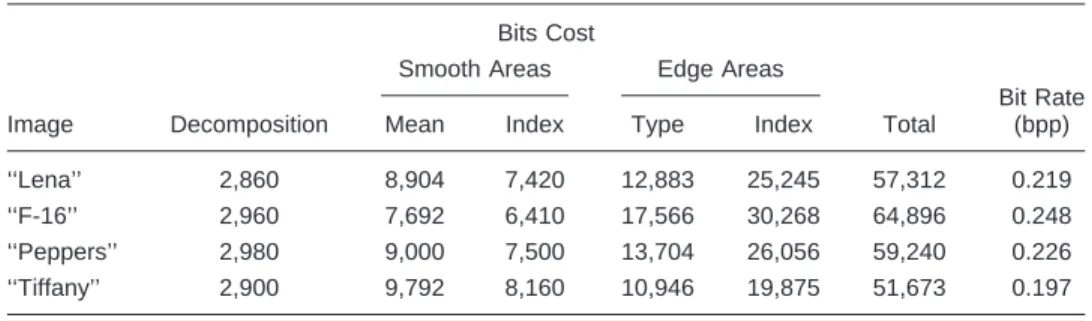
From the experimental results, applying the prediction based on both types and indices can reduce the overall bit rate from 0.03 to 0.05 bpp, i.e., prediction can save about 15 to 25% of storage space required for edge areas. De-tailed bit rate reductions in the edges for the test images are listed in Table 5. Table 6 shows details of the overhead of bit allocation of smooth, edge, and decomposition overhead for the four test images.

The effect of the postprocessing filter applied is shown in Figs. 8 and 10. Figure 8 is the reconstructed image ‘‘Lena’’ without filtering, which displays a slight blocky effect in the smooth regions. Figure 10 is the filtered image. The quality improvements in terms of PSNR caused by filter are listed in Table 7.

The performance of proposed VQ is superior to that of full-search VQ in conjunction with variable length coding abbreviated as VQ-VLC, and the search order coding15共SOC兲 as well. It is also better than SMVQ, which uses side-match prediction.11 Table 8 shows results with different VQ and JPEG coding schemes for comparison. Refer to the data listed in Table 2, which demonstrates that proposed method outperforms than the result listed in Table 8. Figures 11–13 show the reconstructed images after fil-tering of ‘‘F-16,’’ ‘‘Peppers,’’ and ‘‘Tiffany,’’ respectively. All of them demonstrate good quality in terms of bit rate and PSNR values.

5 Conclusions

A new image coding algorithm using simple decomposition and CVQ quantization is proposed to code still images. First, the encoding process decomposes the image into smooth and edge areas. The smooth areas are divided into 16⫻16 and 8⫻8 blocks, then they are encoded with Table 3 Result of prediction for classification types.

Images Correct Fault Correct Ratio (%)

‘‘Lena’’ 1825 1843 49.8

‘‘F-16’’ 2218 2558 46.4

‘‘Peppers’’ 2016 1948 50.9

‘‘Tiffany’’ 1646 1550 51.5

Table 4 Result of prediction for indices.

Images Blocks Correctly Predicted by Type Blocks to Predict in

Indices Correct Fault

Correct Ratio (%) ‘‘Lena’’ 1825 1715 583 1132 34.0 ‘‘F-16’’ 2218 2039 1118 921 54.8 ‘‘Peppers’’ 2016 1944 809 1135 41.6 ‘‘Tiffany’’ 1646 1480 802 678 54.2

Table 5 Bit rate reduction in edges caused by prediction.

Image

Before Prediction After Prediction Bit Reduced

Bit Rate Reduced

Percentage Reduced

Type Index Type Index Type Index

‘‘Lena’’ 18,340 27,721 12,883 25,245 5,457 2,476 7,033 17.2%

‘‘F-16’’ 23,880 36,371 17,566 30,268 6,314 6,103 12,417 20.6%

‘‘Peppers’’ 19,820 29,867 13,704 26,056 6,116 3,811 9,927 20.0%

Fig. 10 ‘‘Lena’’ reconstructed after filtering; 30.59 dB at 0.219 bpp.

Fig. 11 Reconstructed ‘‘F-16’’; 30.16 dB at 0.248 bpp. Fig. 12 Reconstructed ‘‘Peppers’’; 30.02 dB at 0.226 bpp. Table 6 Bit allocation results of the proposed algorithm.

Bits Cost

Image

Smooth Areas Edge Areas

Bit Rate (bpp)

Decomposition Mean Index Type Index Total

‘‘Lena’’ 2,860 8,904 7,420 12,883 25,245 57,312 0.219

‘‘F-16’’ 2,960 7,692 6,410 17,566 30,268 64,896 0.248

‘‘Peppers’’ 2,980 9,000 7,500 13,704 26,056 59,240 0.226

‘‘Tiffany’’ 2,900 9,792 8,160 10,946 19,875 51,673 0.197

Table 7 Performance of the proposed algorithm.

Image Bit Rate (bpp) PSNR before Filtering (dB) PSNR after Filtering (dB) ‘‘Lena’’ 0.219 30.22 30.59 ‘‘F-16’’ 0.248 29.99 30.16 ‘‘Peppers’’ 0.226 29.76 30.02 ‘‘Tiffany’’ 0.197 28.71 28.92

Table 8 Performance comparison of different VQ systems and JPEG.

Image

JPEG (Ref. 6) ESMVQ (Ref. 12) PRVQ (Ref. 8)

PSNR Bit Rate PSNR Bit Rate PSNR Bit Rate PSNR Bit Rate

‘‘Lena’’ 29.47 dB 0.254 bpp 31.50 dB 0.296 bpp 30.44 dB 0.270 bpp 30.13 dB 0.270 bpp Tai, Wu, and Kuo: Predictive classifier for image vector quantization

MRVQ. CVQ is applied to encode the edge areas. A new classification method, classifying edge patterns into 32 typical types, is proposed for use in the edge areas. Two prediction methods, one used for prediction based on clas-sification types and another for prediction based on indices, are applied to reduce the storage space required by classi-fication types and VQ indices. Finally, a filter is applied to smooth areas of the image to reduce the blocking effect.

Using the method proposed in this paper, both the cor-relations of neighboring pixels and the corcor-relations of neighboring block are exploited to reduce the storage space. The traditional VQ uses the redundancy between pixels. However, the proposed prediction method uses the redundancy among blocks. The proposed prediction method based on classification types has an accuracy ratio of over 80% when applied to an entire image. The accuracy is the best performance we have ever seen from the survey of VQ prediction schemes. While applying the prediction to the edge areas only, the accuracy is nearly 50%.

Our future work is to find a better algorithm to achieve higher prediction accuracy. In addition, the bit rate in smooth regions can be reduced further by the use a trans-form coding such as the discrete cosine transtrans-form 共DCT兲 and wavelet compression.

References

1. A. Gersho and R. M. Gray, Vector Quantization and Signal Compres-sion, Kluwer Academic Press, Boston共1992兲.

2. N. M. Nasrabadi and R. A. King, ‘‘Image coding using vector quan-tization: a review,’’ IEEE Trans. Commun. 36共8兲, 957–971 共1988兲. 3. Y. Linde, A. Buzo, and R. M. Gray, ‘‘An algorithm for vector

quan-tization design,’’ IEEE Trans. Commun. 28共1兲, 84–95 共1980兲. 4. J. Forster, R. M. Gray, and M. O. Dunham, ‘‘Finite-state vector

quan-tization for waveform coding,’’ IEEE Trans. Inf. Theory 31共5兲, 348– 359共1985兲.

5. N. M. Nasrabadi and Y. Feng, ‘‘Image compression using address-vector quantization,’’ IEEE Trans. Commun. 38共12兲, 2166–2173

共1990兲.

6. S. H. Yang and S. S. Yang, ‘‘New classified vector quantization with quadtree segmentation for image coding,’’ in Proc. of ICSP, pp. 1051–1054, IEEE共1996兲.

7. B. Ramamurthi and A. Gersho, ‘‘Classified vector quantization of images,’’ IEEE Trans. Commun. 28共1兲, 84–95 共1980兲.

8. S. A. Rizvi and N. M. Nasrabadi, ‘‘Predictive residual vector quanti-zation,’’ IEEE Trans. Image Process. 4共11兲, 1482–1495 共1995兲. 9. S. A. Rizvi and N. M. Nasrabadi, ‘‘Predictive vector quantization

using constrained optimization,’’ IEEE Signal Process. Lett. 1共1兲, 15–18共1994兲.

10. K. N. Ngan and H. C. Koh, ‘‘Predictive classified vector quantiza-tion,’’ IEEE Trans. Image Process. 1共3兲, 269–280 共1992兲.

11. J. C. Tsai and C. H. Hsieh, ‘‘Predictive vector quantization for image compression,’’ Electron. Lett. 34共24兲, 2325–2326 共1998兲.

12. R. F. Chang and W. M. Chen, ‘‘Adaptive edge-based side-match finite-state classified vector quantization with quadtree map,’’ IEEE Trans. Image Process. 5共2兲, 378–383 共1996兲.

13. Y. G. Wu and S. C. Tai, ‘‘A bit rate reduction technique for vector quantization image data compression,’’ IEICE Trans. Fundam. Elec-tron. Commun. Comput. Sci. E82-A共10兲, 2147–2153 共1999兲. 14. S. C. Tai, Y. G. Wu, and L. S. Huang, ‘‘Markov system for vector

quantization image compression,’’ Opt. Eng. 39共5兲, 1338–1343

共2000兲.

15. C. H. Hsieh and J. C. Tsai, ‘‘Lossless compression of VQ index with search-order coding,’’ IEEE Trans. Image Process. 5共11兲, 1579–1582

共1996兲.

Shen-Chuan Tai received BS and MS de-grees in electrical engineering from the Na-tional Taiwan University, Taipei, in 1982 and 1986, respectively, and a PhD degree in computer science from the National Tsing Hua University, Hsinchu, Taiwan, in 1989. From 1989 to 1997, he was an asso-ciate professor of electrical engineering at the National Cheng Kung University, Tainan, Taiwan. He is now a professor at the same institute. Prof. Tai has published more than 90 papers. His teaching and re-search interests include data compression, DSP VLSI array proces-sor, computerized electrocardiogram processing, multimedia sys-tem, and algorithms.

Yung-Gi Wu received his BS in informa-tion and computer engineering from Chung Yuan Christian University, Chung-Li, Tai-wan, in 1992, and his MS and PhD de-grees in electrical engineering from Na-tional Cheng Kung University, Tainan, Taiwan, in 1994 and 2000, respectively. From 1994 to 1996, he was an officer in the army. He is currently an assistant profes-sor of Information Engineering at the Leader University, Tainan, Taiwan. His re-search interests include image processing, data compression and biomedical signal processing.

I-Sheng Kuo received his BS in electrical engineering from National Sun Yat Sen University, Kaohsiung, Taiwan, in 1997, and his MS in electrical engineering from National Cheng Kung University, Tainan, Taiwan, in 1999. He is currently a PhD stu-dent at the institute of Information Science, National Chiao Tung University, HsinChu, Taiwan. His research interests include im-age processing and data compression. Fig. 13 Reconstructed ‘‘Tiffany’’; 28.92 dB at 0.197 bpp.