A Flexible Three-Phased Object-Oriented Data Mining Approach for
Sequential Transactions
Tzung-Pei Hong, Jung-Song Dong and Wen-Yang Lin
Department of Electrical Engineering National University of Kaohsiung
Kaohsiung, 811, Taiwan, R.O.C.
tphong@nuk.edu.tw, m0945120@mail.nuk.edu.tw, wylin@nuk.edu.tw
Abstract
Recently, the object concept has been very popular and used in a variety of applications, especially for complex data description. In the past, data mining is most commonly used in attempts to induce association rules from transaction data. As to object-oriented data mining, Huang et al proposed an algorithm for finding inter- and intra-class knowledge. This paper will improve it and propose a modified mining algorithm to derive sequential patterns from object-oriented data with more pruning effects. There are three kinds of knowledge to be discovered: sequential inter-class patterns, intra-class association rules and sequential inter-intra patterns. There are three phases in the algorithm, with each for a kind of knowledge. The results from the previous phase can be used to prune candidates in the current phase. The candidates generated will thus become much less than those without pruning. Besides, the approach can be easily modified to stop at an intermediate phase if only the desired kind of knowledge is to be obtained. An example is also given to illustrate the proposed algorithm.
Keywords: association rules, data mining,
object-oriented transaction, inter-class pattern, intra-class itemset.
1. Introduction
Knowledge discovery in databases (KDD) means the application of nontrivial procedures for identifying effective, coherent, potentially useful, and unknown patterns in large databases [8]. The KDD process generally consists of the following three phases [7][11].
(1) Pre-processing: In the real world, the input data may be incomplete, noisy and inconsistent. This phase consists of all the actions taken before the actual data analysis starts [7]. Famili et al thought that pre-processing might be performed on the data for the following reasons: solving problems in data that might prevent us from performing any type of analysis on the data, understanding the nature of the data, performing a more meaningful data analysis, and extracting more meaningful knowledge from a given set of data [7].
(2) Data mining: This phase involves the
application of specific algorithms for extracting patterns or rules from data sets in a particular representation.
(3) Post-processing: This phase translates the discovered patterns into acceptable forms for human beings. It may also make the visualization of extracted patterns possible.
Due to the importance of data mining for KDD, many researchers in the fields of databases and machine learning are primarily interested in this research area because it offers opportunities to discover useful information and important relevant patterns in large databases. It further helps decision-makers easily analyze data and make good decisions regarding the domains concerned.
Recently, the object concept has been very popular and used in various applications such as databases, software engineering, knowledge representations [5][6], geographic information systems and even computer architectures [9][10]. An object represents an instance with several related attributes and methods integrated together.
In the past, data mining is most commonly used in attempts to induce association rules from transaction data. As to object-oriented data mining, Huang et al proposed an algorithm for finding inter-and intra-class knowledge. It was divided into two main phrases, one for intra-object association rules, and the other for inter-object sequential patterns [14]. Two apriori-like procedures were adopted to find the two kinds of rules. In this paper, we will improve it and propose a modified mining algorithm to derive sequential patterns from object-oriented data with more pruning effects. The proposed algorithm is divided into three main phases. The first phase mines sequential inter-class patterns. That is, it discoveries the large sequential patterns among the classes. The second phase mines the intra-class itemsets in individual classes. The third phase uses the results from the above two phases to find the sequential inter-intra patterns. The results from the previous phase can be used to prune candidates in the current phase. The generated candidates will thus become much less than those without pruning. Besides, the approach can be easily modified to stop at an intermediate phase if only the desired kind of knowledge is to be obtained. An example is also given to illustrate the proposed algorithm.
follows. Related mining algorithms are reviewed in Section 2. The object-oriented concept is introduced in Section 3. The proposed data-mining algorithm for object-oriented sequence data is described in Section 4. An example to illustrate the proposed algorithm is given in Section 5. Conclusions are stated in Section 6.
2. Review of related work
s
The goal of data mining is to discover important associations among items such that the presence of some items in a transaction will imply the presence of some other items. To achieve this purpose, Agrawal and his co-workers proposed several mining algorithms based on the concept of large itemsets to find association rules in transaction data [1][2][3][4][13]. They divided the mining process into two phases. In the first phase, candidate itemsets were generated and counted by scanning the transaction data. If the number of an itemset appearing in the transactions was larger than a predefined threshold value (called minimum support), the itemset was considered a large itemset. Itemsets containing only one item were first processed. Large itemsets containing only single items were then combined to form candidate itemsets containing two items. This process was repeated until all large itemsets had been found. In the second phase, association rules were induced from the large itemsets found in the first phase. All possible association combinations for each large itemset were formed, and those with calculated confidence values larger than a predefined threshold (called minimum confidence) were output as association rules.
In addition to proposing methods for mining association rules from transactions of binary values, Agrawal et al. also proposed a method [12] for mining association rules from those with quantitative and categorical attributes. Their proposed method first determined the number of partitions for each quantitative attribute, and then mapped all possible values of each attribute into a set of consecutive integers. It then found large itemsets whose support values were greater than the user-specified minimum support value. These large itemsets were then processed to generate association rules, and rules of interest to users were thus output.
Agrawal and Srikant also proposed the AprioriAll mining approach to mine sequential patterns from a set of transactions [2]. Five phases were included in this approach. In the first phase, the transactions were sorted first by customer IDs as the major key and then by transaction time as the minor key. This phase thus converted the original transactions into customer sequences. In the second phase, the set of all large itemsets were found from the customer sequences by comparing their counts with a predefined support parameter. This phase was similar to the process of mining association rules. Note that when an itemset
occurred more than one time in a customer sequence, it was counted once for this customer sequence. In the third phase, each large itemset was mapped to a contiguous integer and the original customer sequences were transformed into the mapped integer sequences. In the fourth phase, the set of transformed integer sequences were used to find large sequences among them. In the fifth phase, the maximally large sequences were then derived and output to users.
Huang et al proposed an algorithm for mining knowledge from object-oriented data [14]. It was divided into two main phases. The first phase was called the intra-object mining phase, in which the large itemsets associated with the same classes (items) but with different attributes were derived. The phase could find out the association relation within the same kind of objects. Each large itemset found in this phase could thus be thought of as a composite item used in phase 2. The second phase, called the inter-object mining phase, in which the large itemsets from the composite items were obtained to get relationship among different kinds of objects. Both the intra-object and inter-object association rules could thus be easily derived from them. Two apriori-like procedures were adopted to find the two kinds of rules.
3. Object-oriented data sequence
s
An object-oriented data sequence (also called transaction in this paper) includes one or more sequential items (such as web pages), each of which is represented as an object or an instance. Each instance inherits its characteristics from a superior object, called class, which defines the basic structure of objects with common properties, including attributes, default values, and methods. The roles of classes and instances in an object-oriented transaction data are like those that schema and tuples play in a relational database [9].
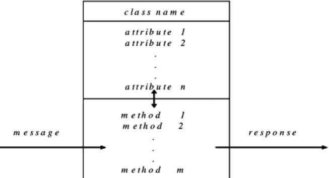
A simple structure of a class is shown in Figure 1, which includes at least three major components: the class name, the attributes and the methods. The class name is an identifier used to identify a class, the attributes are used to represent the characteristics of a class, and the methods are used to implement the operations and functions of a class.
c l a s s n a m e a t t r i b u t e 1 a t t r i b u t e 2 . . . a t t r i b u t e n m e t h o d 1 m e t h o d 2 . . . m e t h o d m m e s s a g e r e s p o n s e c l a s s n a m e a t t r i b u t e 1 a t t r i b u t e 2 . . . a t t r i b u t e n m e t h o d 1 m e t h o d 2 . . . m e t h o d m m e s s a g e r e s p o n s e
An exampleforaclass“wine”isshown in Figure 2 to illustrate the above concept. The class name is specified as“wine”.Theclassincludesfourattributes, on_sale, discount, take_out service and free trial. It also has two methods, confirmation and acknowledgement. wine 1. on_sale 2. discount 3. take_out service 4. free trial 1. confirmation 2. acknowledgement wine 1. on_sale 2. discount 3. take_out service 4. free trial 1. confirmation 2. acknowledgement Figure 2: Anexampleoftheclass“wine”
In this paper, each item itself (such as a web page) is thought of as an class and each item instance appearing in a transaction is thought of as an object. Objects with the same class (item name) may have different attribute values since they may appear in different transactions.
4.
The
proposed
algorithm
for
object-oriented transaction data
In this section, an algorithm is proposed for discovering useful knowledge from object-oriented transaction data. It is an improved version of Huang et al’sforobject-oriented data mining. There are three kinds of knowledge to be discovered: sequential inter-class patterns, intra-class association rules and sequential inter-intra patterns. There are three phases in the algorithm, with each for a kind of knowledge.In this paper, objects (browsed web pages) and attributes are assumed to be binary, with the number 1 representing that the objects and the desired attributes appear. The proposed algorithm can be divided into three main phases. The first phase mines sequential inter-class patterns. That is, it discovers the large sequential patterns among the classes. The second phase mines the intra-class itemsets in individual classes. The third phase uses the results from the above two phases to find the sequential inter-intra patterns.
The results from the previous phase can be used to prune candidates in the current phase. The generated candidates will thus become much less than those without pruning. Besides, the approach can be easily modified to stop at an intermediate phase if only the desired kind of knowledge is to be obtained. That is, the algorithm can stop at Phase 1 for getting only sequential inter-class patterns or at Phase 2 for getting intra-class association rules. It can thus provideaflexibleway according to users’desires.
Before the algorithm is introduced, the notation used in this algorithm is first listed below.
n: the number of transactions; w: the number of classes (web pages); Ij: the j-th class, 1≦j≦w;
mj: the number of attributes for the j-th class (Ij); Ajk: the k-th attribute in the j-th class, 1≦k≦mj,
1≦j≦w;
countj: the count of Ij; countjk: the count of Ajk; supportj: the support of Ij; supportjk: the support of Ajk; α:the predefined minimum support; λ: the predefined minimum confidence;
Cr: the set of sequential inter-class candidate patterns
with r classes;
Lr: the set of large sequential inter-class patterns with r classes;
'
z
C : the set of intra-class candidate itemsets with z
attributes in the same class; '
z
L : the set of large intra-class itemsets with z attributes in the same class;
'' t
C: the set of sequential inter-intra candidate patterns with t composite items;
''
t
L: the set of large sequential inter-intra patterns with
t composite items.
The details of the proposed algorithm are described below.
The proposed three-phased object-oriented data mining algorithm:
INPUT: A set of w classes (items) with mj
attributes, 1≦j≦w, a body of n transaction data, each with some objects derived from the classes and their attribute values, a predefined minimum support value
α,and a predefined confidence value λ.
OUTPUT: A set of object-oriented sequential
patterns.
Phase 1: Find the inter-class relationships
Step 1: Calculate the number (countj) of each
class Ijappearing in the n transaction data, where Ijis
the j-th class, 1≦j≦w; If one class appears more than once in a transaction, count its occurrence only once; Set the support (supportj) of each class Ijas countj/n.
Step 2: Check whether the support of each class Ij
is larger than or equal to the predefined minimum support value α. If Ij satisfies the condition, put it in
the set of large sequential inter-class 1-patterns (L1).
That is,
L1= {Ij| countj/n≧α,1≦j≦w}.
Step 3: If L1 is null, then exit the algorithm;
otherwise, do the next step.
in the sequential inter-class patterns currently being processed.
Step 5: Generate the sequential inter-class
candidate set Cr+1by joining Lr.
Step 6: Calculate the number (counts) of each
sequential inter-class candidate (r+1)-pattern s in Cr+1;
set its support (supports) as counts/n.
Step 7: Check whether the support of each
sequential inter-class candidate (r+1)-pattern s is larger than or equal to the predefined minimum support value α. If s satisfies the condition, put it in the set of large sequential inter-class (r+1)-patterns (Lr+1). That is,
Lr+1= {s | counts/n ≧ α, sCr+1}.
Step 8: If Lr+1is null, do the next step; otherwise,
set r = r +1 and repeat Steps 5 to 7.
Phase 2: Find the intra-class relationships
Step 9: For each large sequential inter-class
1-pattern Ij, calculate the count (countjk) of its each
attribute Ajk, 1≦k≦mj, where mj is the number of
attributes for Ij; Set the support (supportjk) of Ajkas
countjk/n. If Ajk appears more than once in a
transaction, count it only once.
Step 10: Check whether the support of each
attribute Ajkis larger than or equal to the predefined
minimum support value α. If Ajksatisfies the condition,
put it in the set of large intra-class 1-itemsets ( ' 1 L ). That is, ' 1 L = {Ij. Ajk| countjk/nα,IjL1, 1kmj}. Step 11: If ' 1
L is null, then exist the algorithm; otherwise, do the next step.
Step 12: Set z = 1, where z is the number of
attributes in the intra-class itemsets currently being processed.
Step 13: Generate the intra-class candidate
itemset by joining, and remove those without their class relation existing in the large sequential inter-class patterns.
Step 14: Calculate the number (counts) of each
intra-class candidate (z+1)-itemset s in ' 1 z
C ; set its support (supports) as counts/n.
Step 15: Check whether the support of each
intra-class candidate (z+1)-itemset s is larger than or equal to the predefined minimum support value α. If s satisfies the condition, put it in the set of large intra-class (z+1)-itemsets ( ' 1 z L ). That is, ' 1 z L = {s | counts/nα,sC }.'z1 Step 16: If ' 1 z
L is null, do the next step; otherwise, set z = z +1 and repeat Steps 13 to 15.
Phase 3: Find the inter-intra class relationships Step 17: Each large intra-class itemset found so
far is then thought of as a composite item and is put in the large sequential inter-intra 1-pattern ( ''
1
L ).
Step 18: Set t = 1, where t is used to represent the
number of composite items in the sequential inter-intra patterns currently being processed.
Step 19: Generate the sequential inter-intra
candidate set by joining, and remove those without their class relations existing in the large sequential inter-class (t+1) patterns.
Step 20: Calculate the number (counts) of each
sequential inter-intra candidate (t+1)-pattern s in; Set the support (supports) of each s as counts/n.
Step 21: Check whether the support of each
sequential inter-intra candidate (t+1)-pattern s is larger than or equal to the predefined minimum support value α. If s satisfies the condition, put it in the set of large sequential inter-intra (t+1)-patterns ( ''
1 t L ). That is, '' 1 t L = {s | counts/nα,sCt''1}. Step 22: If '' 1 t
L is null, do the next step; otherwise, set t = t + 1 and repeat Steps 19 to 21.
Finding the Outputs:
Step 23: Derive the maximally sequential inter-class patterns from L2to Lr.
Step 24: Derive the intra-class association rules
with confidence values larger than or equal to λfrom
' 2
L to ' z
L .
Step 25: Derive the maximally sequential inter-intra patterns from ''
2
L to L .''t
After Step 25, the three kinds of object-oriented knowledge are found from the given set of data.
5. An Example
In this section, an example is given to illustrate the proposed three-phased object-oriented data mining algorithm. This is a simple example to show how the proposed algorithm can be used to generate the association rules from object-oriented data. Assume there are several classes, with each being a web page. Each class consists of its own attributes (e.g. a take_out service) related to its corresponding web page. A browsed web page in a transaction is thus an object generated from a certain class. In this example, we assume there are five classes (web pages), I1to I5.
The browsed web pages from the same class in the transactions have the same attributes and the ones from different classes may have different attributes. Here, for simplicity, we assume all the classes have four attributes. Note that the proposed approach can
handle the classes with different attributes.
Let Aij denote the j-th attribute for the i-th class
(web page). For example, I1 has four different
attributes A11 to A14, I2has four attributes A21to A24,
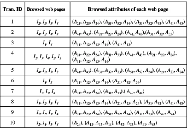
and so on. The value of each attribute is either 0 or 1. Also assume the ten transactions shown in Table 1 are to be processed.
Table 1: The ten browsing data in this example
(A24), (A12, A13, A14), (A32, A33), (A41, A43) I2, I1, I3, I4 10 (A21, A23, A24), (A51, A52, A54), (A31, A33), (A42, A44) I2, I5, I3, I4 9 (A11, A12, A13, A14), (A21, A23, A24), (A31, A32), (A41, A43) I1, I2, I3, I4 8 (A21, A23, A24), (A31, A33),( A42, A44) I2, I3, I4 7 (A11, A12, A13, A14), (A51, A52, A54) I1, I5 6 (A41, A43), (A31, A32, A33), (A51, A52, A54), (A21, A23, A24) I4, I3, I5, I2 5 (A21, A22, A24), (A31, A33), (A41, A43), (A21, A22, A24), (A11, A12, A13, A14) I2, I3, I4, I2, I1 4 (A11, A12, A13, A14), (A41, A43) I1, I4 3 (A41, A43), (A21, A22, A24), (A41,A43),(A31, A32, A33) I4, I2, I4, I3 2 (A21, A23, A24), (A51, A52, A54), (A31, A32, A33), (A41, A43) I2, I5, I3, I4 1
Browsed attributes of each web page
Browsed web pages
Tran. ID (A24), (A12, A13, A14), (A32, A33), (A41, A43) I2, I1, I3, I4 10 (A21, A23, A24), (A51, A52, A54), (A31, A33), (A42, A44) I2, I5, I3, I4 9 (A11, A12, A13, A14), (A21, A23, A24), (A31, A32), (A41, A43) I1, I2, I3, I4 8 (A21, A23, A24), (A31, A33),( A42, A44) I2, I3, I4 7 (A11, A12, A13, A14), (A51, A52, A54) I1, I5 6 (A41, A43), (A31, A32, A33), (A51, A52, A54), (A21, A23, A24) I4, I3, I5, I2 5 (A21, A22, A24), (A31, A33), (A41, A43), (A21, A22, A24), (A11, A12, A13, A14) I2, I3, I4, I2, I1 4 (A11, A12, A13, A14), (A41, A43) I1, I4 3 (A41, A43), (A21, A22, A24), (A41,A43),(A31, A32, A33) I4, I2, I4, I3 2 (A21, A23, A24), (A51, A52, A54), (A31, A32, A33), (A41, A43) I2, I5, I3, I4 1
Browsed attributes of each web page
Browsed web pages
Tran. ID
In Table 1, A11 represents that the value of the
attribute A11 in the web page I1 is 1. If A11 doesn’t
appear in the table, its value is 0. Only the association relations among the appearing attribute behaviors (i.e. the value is 1) are to be found. The proposed algorithm can also be easily to extended to find relations for non-appearing attribute behaviors. For the browsing data in Table 1, the proposed three-phased object-oriented data mining algorithm proceeds as follows.
Step 1: The count value of each class (web page)
appearing in the ten transaction data is first calculated. Take the class I1 as an example. Its count value =
(0+0+1+1+0+1+0+1+0+1) = 5. This step is repeated for the other web pages, with the results show in Table 2.
Table 2: The count of each web page in Table 1
4 9 8 8 5 Count 0 1 1 1 1 10 1 1 1 1 0 9 0 1 1 1 1 8 0 1 1 1 0 7 1 0 0 0 1 6 1 1 1 1 0 5 0 1 1 1 1 4 0 1 0 0 1 3 0 1 1 1 0 2 1 1 1 1 0 1 I5 I4 I3 I2 I1 Trans ID. 4 9 8 8 5 Count 0 1 1 1 1 10 1 1 1 1 0 9 0 1 1 1 1 8 0 1 1 1 0 7 1 0 0 0 1 6 1 1 1 1 0 5 0 1 1 1 1 4 0 1 0 0 1 3 0 1 1 1 0 2 1 1 1 1 0 1 I5 I4 I3 I2 I1 Trans ID.
The support of each class can be derived by its count value over the number of transaction data. In this example, the number of transaction data is 10.
Step 2: The support of each class is checked to
determine whether it is larger than or equal to the predefined minimum support value α. Assume in this example, the minimum support is set at 0.6. Since the support values of I2, I3and I4are larger than or equal
to 0.6, the three classes are put in the set of large sequential inter-class 1-patterns L1(Table 3).
Table 3: The set of large sequential inter-class
1-patterns L1in this example
9/10 I4 8/10 I3 8/10 I2 Support Sequential 1-pattern 9/10 I4 8/10 I3 8/10 I2 Support Sequential 1-pattern
Step 3: If L1is null, then the algorithm is exited;
otherwise the next step is done. In this example, since
L1is not null, Step 4 is then executed.
Step 4: The variable r is set at 1, where r is the
number of classes in the sequential inter-class 1-pattern currently being processed.
Step 5: The sequential inter-class candidate set Cr+1is formed by joining Lr. C2is first generated from L1as follows: (I2, I2), (I2, I3), (I2, I4), (I3, I2), (I3, I3), (I3, I4), (I4, I2), (I4, I3) and (I4, I4).
Step 6: The count of each sequential inter-class
candidate pattern s in C2is calculated. The results are
shown in Table 4.
Table 4: The count of each sequential inter-class
candidate pattern in C2 1 (I4, I4) 2 (I4, I3) 3 (I4, I2) 6 (I3, I4) 0 (I3, I3) 2 (I3, I2) 7 (I2, I4) 7 (I2, I3) 1 (I2, I2) Count Sequential inter-class candidate 2-pattern 1 (I4, I4) 2 (I4, I3) 3 (I4, I2) 6 (I3, I4) 0 (I3, I3) 2 (I3, I2) 7 (I2, I4) 7 (I2, I3) 1 (I2, I2) Count Sequential inter-class candidate 2-pattern
The support of each candidate s in C2 is then
calculated as its count divided by 10.
Step 7: The support of each sequential inter-class
candidate 2-pattern is then compared with the predefined minimum support value 0.6. In this example, the three sequential inter-class candidate 2-patterns (I2, I3), (I2, I4) and (I3, I4) are larger than or
equal to 0.6. They are thus kept in L2(Table 5).
Step 8: If Lr+1 is null, the next step is done;
otherwise, r = r + 1 and Steps 5 to 7 are repeated. Since L2 is not null in the example, r = r + 1 = 3.
Steps 5 to 7 are repeated to get L3. C3 is then
generated from L2, and the sequential inter-class
formed. Their supports are calculated as 0.6 and 0.1, respectively. Since only the sequential inter-class candidate 3-pattern (I2, I3, I4) is larger than 0.6, it is
put in L3. In this example, no sequential inter-class
candidate 4-patterns can be formed. L4is thus null and
the next step then begins.
Table 5: The large sequential 2-patterns kept in L2
6/10 (I3, I4) 7/10 (I2, I4) 7/10 (I2, I3) Support Sequential inter-class 2-pattern 6/10 (I3, I4) 7/10 (I2, I4) 7/10 (I2, I3) Support Sequential inter-class 2-pattern
Step 9: The count value of each attribute in each
large sequential inter-class 1-pattern is calculated. In this example, the three classes I2, I3and I4are large, so
only the count values of the attributes for the three classes are calculated. Take the attribute A21 for the
class I2 as an example. Its count value is
(1+1+0+1+1+0+1+1+1+0), which is 7. This step is repeated for the other attributes, with the results shown in Table 6.
The support of each attribute can be derived by its count value over the number of transaction data. In this example, the number of transaction data is 10.
Step 10: The support of each attribute is checked
to determine where it is larger than or equal to the predefined minimum support value α, which is 0.6 in this example. Since A21, A24, A31, A33, A41 and A43
satisfy the condition, these attributes are put in the set of large sequential intra-class 1-patterns (Table 7).
Table 6: The count of each attribute in I2, I3and I4
2 7 2 7 0 7 5 7 8 5 2 7 count 0 1 0 1 0 1 1 0 1 0 0 0 10 1 0 1 0 0 1 0 1 1 1 0 1 9 0 1 0 1 0 0 1 1 1 1 0 1 8 1 0 1 0 0 1 0 1 1 1 0 1 7 0 0 0 0 0 0 0 0 0 0 0 0 6 0 1 0 1 0 1 1 1 1 1 0 1 5 0 1 0 1 0 1 0 1 1 0 1 1 4 0 1 0 1 0 0 0 0 0 0 0 0 3 0 1 0 1 0 1 1 1 1 0 1 1 2 0 1 0 1 0 1 1 1 1 1 0 1 1 A44 A43 A42 A41 A34 A33 A32 A31 A24 A23 A22 A21 I4 I3 I2 Tran. ID 2 7 2 7 0 7 5 7 8 5 2 7 count 0 1 0 1 0 1 1 0 1 0 0 0 10 1 0 1 0 0 1 0 1 1 1 0 1 9 0 1 0 1 0 0 1 1 1 1 0 1 8 1 0 1 0 0 1 0 1 1 1 0 1 7 0 0 0 0 0 0 0 0 0 0 0 0 6 0 1 0 1 0 1 1 1 1 1 0 1 5 0 1 0 1 0 1 0 1 1 0 1 1 4 0 1 0 1 0 0 0 0 0 0 0 0 3 0 1 0 1 0 1 1 1 1 0 1 1 2 0 1 0 1 0 1 1 1 1 1 0 1 1 A44 A43 A42 A41 A34 A33 A32 A31 A24 A23 A22 A21 I4 I3 I2 Tran. ID Step 11: If ' 1
L is null, the algorithm is exited; otherwise the next step is done. In this example, '
1
L is not null, such that the next step is executed.
Step 12: z is set at 1, where z is the number of
attributes in the intra-class itemsets currently being processed.
Step 13: The intra-class candidate itemset '
1 z C is generated by joining ' z
L under the condition that each (z+1)-itemset must have the same class. '
2
C is
first generated from ' 1
L as follows : (A21), (A24), (A31),
(A33), (A41) and (A43).
Table 7: The set of large intra-class 1-patterns
7/10 A43 7/10 A41 7/10 A33 7/10 A31 8/10 A24 7/10 A21 Support Sequential intra-class 1-patterns 7/10 A43 7/10 A41 7/10 A33 7/10 A31 8/10 A24 7/10 A21 Support Sequential intra-class 1-patterns
Step 14: The count of each intra-class candidate
2-itemset in ' 2
C is calculated, with the results shown in Table 8. The support of each intra-class candidate itemset is derived by its count over 10.
Step 15: The support of each intra-class candidate itemset is compared with the predefined minimum support value 0.6. In this example, the 3 itemsets, (A21, A24), (A31, A33) and (A41, A43) satisfy the
condition and are kept in ' 2
L . Table 9 shows the
results.
Table 8: The count results of the intra-class candidate
2-itemsets in ' 2 C 7 (A41,A43) 6 (A31,A33) 7 (A21, A24) Count Intra-class Itemset 7 (A41,A43) 6 (A31,A33) 7 (A21, A24) Count Intra-class Itemset
Table 9: The large intra-class itemsets in '
2 L 7/10 (A41,A43) 6/10 (A31,A33) 7/10 (A21, A24) Support Itemset 7/10 (A41,A43) 6/10 (A31,A33) 7/10 (A21, A24) Support Itemset Step 16: If ' 1 z
L is null, the next step is done; otherwise, z = z + 1 and Steps 13 to 15 is repeated. Since '
2
L is not null in this example, Steps 13 to 15 is then repeated to find '
3
L .In this example, '
3
C is null, such that the next step is done.
Step 17: Each large itemset found so far is
thought of as a composite item and is put in the large 1-sequence ( ''
1
L ). In this example, the large itemsets
found so far include (A21), (A24), (A31), (A33), (A41),
(A43), (A21, A24), (A31,A33) and (A41,A43). Each of them
is thought of as a composite item.
Step 18: t is set at 1, where t is the number of
composite items in the sequential inter-intra patterns currently being processed.
Step 19: The inter-intra candidate set ''
1
t
generated by joining '' t
L and '' t
L under the condition that t-1 items in the two sequences to be joined are the same and with the same orders. Different permutations represent different candidates. Besides, the candidates without their class relations existing in the large sequential inter-class (t+1)-patterns are removed. For example, the sequential inter-class 2-patterns found in Phase 1 are (I2, I3), (I2, I4) and (I3, I4). The sequential inter-intra 2-pattern (A31, A24) will
thus not be generated as a candidate since (I3, I2) is
not in the inter-class 2-patterns. Through this kind of pruning, the generated candidates will become much less than those without pruning.
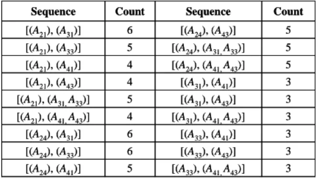
Step 20: The number (counts) of each sequential
inter-intra candidate (t+1)-pattern s in '' 1 t
C is calculated. The count of each sequence inter-intra 2-candidate is shown in Table 10. The support of each candidate s in ''
2
C is then calculated as its count divided by 10.
Table 10: The count results of each sequential
inter-intra candidates in '' 2 C 3 [(A33), (A41,A43)] 5 [(A24), (A41)] 3 [(A33), (A43)] 6 [(A24), (A33)] 3 [(A33), (A41)] 6 [(A24), (A31)] 3 [(A31), (A41,A43)] 4 [(A21), (A41,A43)] 3 [(A31), (A43)] 5 [(A21), (A31,A33)] 3 [(A31), (A41)] 4 [(A21), (A43)] 5 [(A24), (A41,A43)] 4 [(A21), (A41)] 5 [(A24), (A31,A33)] 5 [(A21), (A33)] 5 [(A24), (A43)] 6 [(A21), (A31)] Count Sequence Count Sequence 3 [(A33), (A41,A43)] 5 [(A24), (A41)] 3 [(A33), (A43)] 6 [(A24), (A33)] 3 [(A33), (A41)] 6 [(A24), (A31)] 3 [(A31), (A41,A43)] 4 [(A21), (A41,A43)] 3 [(A31), (A43)] 5 [(A21), (A31,A33)] 3 [(A31), (A41)] 4 [(A21), (A43)] 5 [(A24), (A41,A43)] 4 [(A21), (A41)] 5 [(A24), (A31,A33)] 5 [(A21), (A33)] 5 [(A24), (A43)] 6 [(A21), (A31)] Count Sequence Count Sequence
Step 21: The support of each sequential inter-intra candidate pattern is then compared with the predefined minimum support value 0.6. In this example, the three sequential inter-intra 2-patterns shown in Table 11 satisfy the condition and are kept in ''
2
L.
Table 11: The large sequential inter-intra 2-patterns in
'' 2 L 6/10 [(A24), (A33)] 6/10 [(A24), (A31)] 6/10 [(A21), (A31)] Support Sequence 6/10 [(A24), (A33)] 6/10 [(A24), (A31)] 6/10 [(A21), (A31)] Support Sequence Step 22: If '' 1 t
L is null, the next step is done; otherwise, t = t + 1 and Steps 19 to 21 are repeated. Since ''
2
L is not null in the example, t = 2 + 1 = 3. Steps 19 to 21 are thus repeated to find ''
3 L . No sequential inter-intra candidate 3-patterns are formed in this example.
Step 23: The maximally sequential inter-class
patterns are derived from L2to Lr. For example, (I2, I3, I4) is one of the maximally sequential inter-class
patterns.
Step 24: The intra-class association rules with
confidencevalueslargerthan orequalto λ arederived from '
2
L to L .'z Forexample,“If (I4= A43), then (I4=
A41) with a confidence factor of 1”is one of the
intra-class association rules.
Step 25: The maximally sequential inter-intra
patterns are derived from '' 2
L to '' t
L. For example, ((I2
= A21), (I3= A31)) is one of the maximally sequential
inter-intra patterns.
6. Conclusions
Thispaperhasimproved Huang etal’sapproach for object-oriented data mining from sequential transactions. The modified mining algorithm can discover sequential patterns from object-oriented data with more pruning effects. Objects (browsed web pages) and attributes are assumed to be binary, with the number 1 representing that the objects and the desired attributes appear. The proposed algorithm can be divided into three main phases. The first phase mines sequential inter-class patterns. The second phase mines the intra-class itemsets in individual classes. The third phase uses the results from the above two phases to find the sequential inter-intra patterns. The results from the previous phase we will can be used to prune candidates in the current phase. Besides, the proposed approach provides a flexible way for users’ desires. An example has also been given to illustrate the proposed algorithm. In the future, we will attempt to study the implementation issues, such as using appropriate data structures, to make the concepts more practical.
7. References
[1] R. Agrawal, and R. Srikant,“Fastalgorithm for mining association rules”, The international
conference on very large databases, pp.
487–499, 1994.
[2] R. Agrawal, and R. Srikant,“Mining sequential
patterns”, The eleventh international
conference on data engineering, pp. 3–14, 1995.
[3] R. Agrawal, T. Imielinksi and A. Swami, “Mining association rulesbetween setsofitems
in large database”, The ACM SIGMOD
conference, 1993.
[4] R. Agrawal, T. Imielinksi and A. Swami, “Databasemining:aperformanceperspective”,
IEEE Transactions on Knowledge and Data
Engineering, pp. 914–925, 1993.
[5] C. Clair, C. Liu, and N. Pissinou, “Attribute weighting: a method of applying domain knowledge in the decision tree process”, The
seventh international conference on information
1998.
[6] P. Clark and T. Niblett, “The CN2 induction algorithm”, Machine Learning, Vol. 3, NO. 4, pp. 261-283, March 1989.
[7] A. Famili, W. M. Shen, R. Weber and E. Simoudis,“Data preprocessing and intelligent dataanalysis”, Intelligent Data Analysis, Vol.
1, pp. 3-23, 1997.
[8] W. J. Frawley, G. Piatetsky-Shapiro and C. J. Matheus, “Knowledge discovery in databases: an overview”, The AAAI workshop on
knowledge discovery in databases, pp. 1–27,
1991.
[9] W. Kim,“Object-oriented databases: definition and research directions”, IEEE Transactions on
Knowledge and Data Engineering, Vol. 2, NO. 3,
pp. 327–341, 1990.
[10] T. D. Kimura,“Object-oriented dataflow”, The
11th IEEE international symposium on visual
languages, pp. 180–186, 1995.
[11] H. Mannila, “Methods and problems in data
mining”, The international conference on
database theory, pp. 41-55, 1997.
[12] R. Srikant, and R. Agrawal, “Mining quantitative association rules in large relational
tables”, The ACM SIGMOD international
conference on management of data, pp. 1–12,
1996.
[13] R. Srikant, Q. Vu and R. Agrawal, ”Mining association ruleswith item constraints,”In The third international conference on knowledge discovery in databases and data mining, pp.
67–73, 1997.
[14] C. M. Huang, T. P. Hong and S. J. Horng, “Mining knowledge from object-oriented instances”, Expert System with Applications, Vol. 33, NO. 2, pp. 441-450, August 2007.
8. Acknowledgment
This research was supported by the National Science Council of the Republic of China under contract NSC 95-2221-E-390-025.