探索市場波動度在技術分析中所提供的訊息

行政院國家科學委員會專題研究計畫 成果報告

探索市場波動度在技術分析中所提供的訊息

研究成果報告(精簡版)

計 畫 類 別 ： 個別型 計 畫 編 號 ： NSC 100-2410-H-004-051- 執 行 期 間 ： 100 年 08 月 01 日至 101 年 07 月 31 日 執 行 單 位 ： 國立政治大學國際經營與貿易學系 計 畫 主 持 人 ： 林信助 共 同 主 持 人 ： 郭炳伸 計畫參與人員： 碩士班研究生-兼任助理人員：范瑋凌 碩士班研究生-兼任助理人員：高育幸 博士班研究生-兼任助理人員：吳家豪 報 告 附 件 ： 出席國際會議研究心得報告及發表論文 公 開 資 訊 ： 本計畫可公開查詢

中 華 民 國 101 年 09 月 05 日

中 文 摘 要 ： 這個研究計畫主要在研究市場波動度是否可以提升技術交易 法則的獲利性。 切確而言，我們比較能夠包含市場波動度訊 息的變動型移動平均法則， 以及其他五種不包含市場波動度 訊息的技術交易法則。 利用道瓊工業指數的資料以及 Hansen (2005)所提出的卓越預測能力檢定法， 我們發現變 動型移動平均法則在獲利性上表現的比他五種技術交易法則 來得好。 同時，透過 Cumby and Modest(1987)的檢定， 我 們也發現變動型移動平均法則較佳的獲利能力可能是來自於 其較好的市場擇時能力。 此外，我們研究變動型移動平均法 則較好的表現是否會因為不同的市場狀況而改變， 並發現了 兩個有趣的現象。 首先，變動型移動平均法則在牛市與熊市 的市場擇時能力是不對稱的。 第二，變動型移動平均法則在 熊市時的表現與一般的移動平均法則類似；但在牛市時， 變 動型移動平均法則的表現肯定勝過一般的移動平均法則。 中文關鍵詞： 技術分析；變動型移動平均；資料窺探偏誤； 市場波動度 英 文 摘 要 ： This project investigates whether market volatility is valuable in enhancing profitability of technical trading rules. Specifically, we compare performance of the Variable Moving Average (VMA) rule, which incorporates market volatility information, with five other popular trading rules without market volatility information. When applied to the Dow Jones Industrial Average index, the Superior Predictive Ability test by Hansen (2001) shows that the VMA rule outperforms other rules in profitability. With the test of Cumby and Modest (1987), we find that the better

profitability of the VMA rule might have come from its better market timing ability. Furthermore, we explore whether the better performance of the VMA rule is sensitive to different market conditions, and obtain two interesting results. First, the market timing ability of the VMA rule is asymmetric in bull and bear markets. Second, while the performance of the VMA rule is similar to that of the MA rule in the bear market, the VMA rule certainly outperforms the Moving Average (MA) rule in the bull market.

英文關鍵詞： Technical Analysis, Variable Moving Average, Data Snooping Bias, Market Volatility

行政院國家科學委員會補助專題研究計畫

□期中進度報告

■期末報告

探索市場波動度在技術分析中所提供的訊息

計畫類別：■個別型計畫 □整合型計畫

計畫編號：NSC 100-2410-H-004-051-

執行期間： 100 年 8 月 1 日至 101 年 7 月 31 日

執行機構及系所：國立政治大學國際經營與貿易學系

計畫主持人：林信助

共同主持人：郭炳伸

計畫參與人員：吳家豪（博士生）

、高育幸（碩士生）

、范瑋凌（碩士生）

本計畫除繳交成果報告外，另含下列出國報告，共 _1_ 份：

□移地研究心得報告

■出席國際學術會議心得報告

□國際合作研究計畫國外研究報告

處理方式：除列管計畫及下列情形者外，得立即公開查詢

□涉及專利或其他智慧財產權，□一年□二年後可公開查詢

中 華 民 國 101 年 9 月 4 日

探索市場波動度在技術分析中所提供的訊息

計畫編號 : NSC 100-2410-H-004-051-執行期間 : 中華民國100年8月1日至101年7月31日 主持人: 林信助 (國立政治大學國際經營與貿易學系) E-mail: shjlin@nccu.edu.tw 執行單位 : 國立政治大學國際經營與貿易學系 一、 摘要 這個研究計畫主要在研究市場波動度是否可以提升技術交易法則的獲利性。 切確而言,我們比較 能夠包含市場波動度訊息的變動型移動平均法則, 以及其他五種不包含市場波動度訊息的技術 交易法則。 利用道瓊工業指數的資料以及 Hansen (2005) 所提出的卓越預測能力檢定法, 我們 發現變動型移動平均法則在獲利性上表現的比他五種技術交易法則來得好。 同時, 透過 Cumby and Modest(1987)的檢定,我們也發現變動型移動平均法則較佳的獲利能力可能是來自於其較 好的市場擇時能力。 此外,我們研究變動型移動平均法則較好的表現是否會因為不同的市場狀況 而改變, 並發現了兩個有趣的現象。 首先, 變動型移動平均法則在牛市與熊市的市場擇時能力是 不對稱的。 第二,變動型移動平均法則在熊市時的表現與一般的移動平均法則類似;但在牛市時, 變動型移動平均法則的表現肯定勝過一般的移動平均法則。 關鍵詞: 技術分析; 變動型移動平均;資料窺探偏誤; 市場波動度 Abstract

This project investigates whether market volatility is valuable in enhancing profitability of technical trading rules. Specifically, we compare performance of the Variable Moving Average (VMA) rule, which incorporates market volatility information, with five other popular trading rules without market volatility information. When applied to the Dow Jones Industrial Average index, the Superior Predictive Ability test by Hansen (2001) shows that the VMA rule outperforms other rules in profitability. With the test of Cumby and Modest (1987), we find that the better profitability of the VMA rule might have come from its better market timing ability. Furthermore, we explore whether the better performance of the VMA rule is sensitive to different market conditions, and obtain two interesting results. First, the market timing ability of the VMA rule is asymmetric in bull and bear markets. Second, while the performance of the VMA rule is similar to that of the MA rule in the bear market, the VMA rule certainly outperforms the Moving Average (MA) rule in the bull market.

Keywords: Technical Analysis, Variable Moving Average, Data Snooping Bias, Market Volatility

二、 緣由與目的

1

Introduction

Technical analysis is a discipline for forecasting price movements through the study of historical data, primarily price and volume. It has been widely employed by practitioners for more than a century (Smidt 1965, Taylor and Allen 1992, Billingsley and Chance 1996, Lui and Mole 1998, Oberlechner 2001, Gehrig and Menkhoff 2004, Covel 2005, Lo and Hasanhodzic 2009.) Despite its widespread adoption by practitioners, the profitability of technical trading rules has presented a serious challenge to the conventional view that markets are at least weak-form efficient. Therefore, whether practitioners can obtain statistically significant profit by employing technical trading rules has drawn continuing attention and discussion since Alexander (1961), and is still under dispute among the academia.

Recently, quite a few empirical studies have emerged to investigate the profitability of technical trading rules from many different perspectives, such as different trading systems / mechanisms, transaction cost consideration, data snooping bias problems, and statistical tests adopted (Brock et al. 1992, Chan et al. 1996, Neely 1997, Sullivan et al. 1999, LeBaron 1999, Lo et al. 2000, Okunev and White 2003, Hsu and Kuan 2005, Schulmeister 2009.) The bulk of these studies seem to indicate that technical trading rules can still help investors predict the market.

Compared to price and volume, market volatility has not been extensively studied in the technical analysis literature, despite its importance in finance such as hedging portfo-lios construction, derivative securities pricing and computing the value-at-risk. A notable exception is the variable moving average (VMA, hereafter) rule proposed by Chande (1992), which is also currently adopted by traders in financial markets. The creation of the VMA rule was motivated by the fact that existing technical trading rules without volatility information are static in the sense that the parameter values of those trading rules are not responsive enough to the ever-changing market condition. For example, a simple moving average (MA, hereafter) trading strategy implies that a fixed window-length of historical data is used in constructing moving averages, and in producing trading signals at all time. In contrast, the VMA rule, as an extension to the popular MA rule, automatically adjusts the effective window-length of each moving average according to the changing market volatility. In other words, the market volatility is built into the VMA rule to better gauge the market condition. As a result, the VMA rule provides a good laboratory to study whether the market volatility is indeed valuable in enhancing the profitability of technical trading rules.

Although the VMA rule has been existing since Chande (1992), it is yet to be thor-oughly scrutinized. In this paper, we specifically propose to compare the performance of the VMA rule with five other most tested trading rules (filter, moving average, sup-port and resistance, channel breakout, and momentum strategies) with the Dow Jones Industrial Average (DJIA) index over the period from 1928/10/1 to 2010/6/28. To min-imize the data snooping bias, our comparison is facilitated with the Superior Predictive Ability (SPA, hereafter) test proposed by Hansen (2005) in full sample as well as several sub-sample periods. The market time ability of various technical trading rules are also

compared with the test proposed by Cumby and Modest (1987). In addition, the market timing ability are investigated both in the bull and the bear markets.

Our empirical results clearly demonstrate that the VMA trading rule outperforms others with statistically significant and larger profitability in the DJIA market. In terms of the market timing ability, there is strong evidence indicating that both the VMA and the MA rules can forecast the direction of future price movement, but the VMA rule does generate higher average profit per trading day. Furthermore, our results show that the VMA rule outperforms the MA rule in the bull market.

The remainder of the paper is organized as follows. Section 2 outlines the technical trading rules examined in this paper. Hansen’s SPA test is constructed and presented in Section 3. Section 4 contains a description of data examined in this paper, and presents results of the SPA tests. In Section 5, we discuss results of the market timing ability test. Section 6 concludes the paper.

三、 結果與討論

2

Technical Trading Rules

The technical trading rules examined in this paper can be categorized into two groups. The first group consolidates the market volatility to form the new moving average system, with the VMA rule being the representative. The second group, in contrast, includes rules without the market volatility information: filter rule (FR), moving average (MA), support and resistance (SR), channel breakout (CB), and the momentum (MOM) strategy. These five technical trading rules are very popular among the practitioners in financial markets and have already drawn a lot of discussion in the literature, Since the VMA rule is less familiar to the academia, we will devote most effort in introducing the VMA rule in this section.

2.1 The VMA Rule

Considering the dynamic changing nature of the market, Chande (1992) introduces the VMA rule which can adapt itself to the market condition, namely becoming a shorter moving average as the market is trending, while automatically changing into a longer moving average when the market is ranging. Specifically, the VMA rule is constructed by revising the following exponential moving average rule,

EMAt = αPt+ (1 − α)EMAt−1, (1)

α = 2

N + 1,

where EMAt is the exponential moving average value at time t; α, often referred as

the smoothing parameter, is a numerical constant which describes the weight that the exponential moving average gives to the more recent data; N is the effective length of

historical data used to calculate the exponential moving average value; Pt is the closing

price at time t. As the smoothing parameter α increases (N decreases), the exponential moving average adopts a shorter length of historical data and places more weight on the most recent data; it will therefore trace the market price more closely. In contrast, as α decreases (N increases), a longer length of historical data is considered, and greater weight is given to the more distant data. Consequently, the deviation of the exponential moving average from the actual price series increase. Since α is a fixed constant in this traditional VMA rule, it does not adjust to the changing market market. Therefore, Chande (1992) suggests replacing the constant smoothing parameter, α, with a variable which is tied up to a market-condition related variable as below:

VMAt = α∗tPt+ (1 − α∗t)VMAt−1, (2)

α∗_t = αVRt,

where VMAtis the variable moving average at time t; the smoothing parameter α∗t here is

time-varying, consists of a constant term α and the market volatility ratio, VRt≡ σtn/σ ref t ,

which is by the standard deviation, σn

t, of closing prices over past n periods at time t, and

the reference standard deviation, σ_tref, of closing prices over some period of time longer than n at time t.

2.1.1 Trading Strategies for the VMA Rule

For trading strategies in the VMA rule, Chande suggests that all conventional strategies with the moving average system can be extended in the VMA. The most popular trading strategy is the moving average crossover decision model : buy when current price (shorter VMA) moves above the VMA (longer VMA); while sell when current price (shorter VMA)

moves below the VMA (longer VMA).1

3

Empirical Results on the Trading Rule Profitability

3.1 Data

Data examined in this paper consists of the Dow Jones Industrial Average (DJIA) daily closing price from Oct 1, 1928 to June 28, 2010 - a collection of more than 80 years of daily data.

3.2 SPA Test Results: Full Sample and Sub-samples

In this subsection, we present the SPA test results on the profitability of 5,162 technical trading rules. Table 1 reports the performance of the best trading rule on each trading family in the full sample with the one-way transaction cost 0.05%. The first and second columns in Table 1 are the best rules on each trading family, and their rank in the universe of trading rules. The third, fourth, and fifth columns are their total number of trades, daily mean return and annualized return they obtain in this period. The last column reports the p−value of SPA test. We can observe that the overall best rule in the universe 1_{For the parameter values of the VMA, the setting in Chande (1992) is adopted. We also consider the}

suggestions from the websites of professional trading companies.

is the VMA family, and the best rule of the MSV wins the third place. The annual profits are 8.18%, 7.64%, 7.04%, 6.67%, 4.98%, and 2.64%, respectively, for the best rule of the VMA, MSV, MA, FR, CB, and the SR families. The best rule of the VMA, MSV, MA and FR families enjoy statistically significant profit at the 10% significant level, while profits from other two type of rules are all insignificant different from 0. To sum up the SPA test results for the full sample, as presented in Table 1 , we find that the VMA rule can earn statistically and economically significant profit, and it outperforms others with highest mean return.

Table 2 describes the performance of the best rule on each trading family in the sub-samples. Panel A and B demonstrate the results in the first and second sub-sample, respectively. Similarly, the best rule in the universe in these two sub-samples are all the VMA rules. It has economically significant profitability due to its SPA p−value less than 5% in the first sub-sample. Except for the best rule of the VMA and MSV, other rules are insignificantly profitable in the first sub-sample. And in the second sub-sample, the profitability of all types of rule is weaker. We reject the null hypothesis for the performance of the best rule on the VMA family only at the 10% significant level.

Table 3 summarizes the performance of the technical trading rules in other five

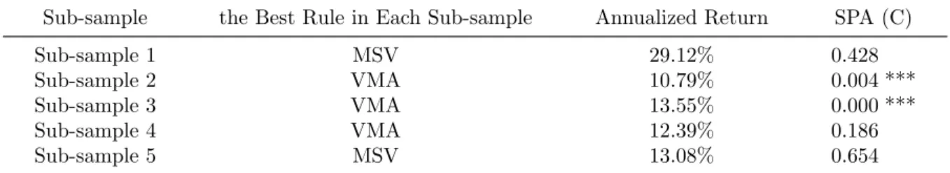
sub-samples. We just report the best one in the universe of 5,162 trading rules in each

sub-sample with its annualized return and the SPA p−value. We can discover that three out of five best rules in these periods are the VMA rules (Sub-sample 2, 3, and 4), and the null hypothesis of the SPA test for Sub-sample 2 and 3 can be rejected even at 1% significant level. Although the best one in the Sub-sample 1 and 5 are the MSV rule, their profitability are all insignificant.

To conclude the SPA results both for the full sample and all sub-samples, we can find that the performance of the VMA is more outstanding than other five rules. Besides, these results provide us the evidence that the information of market volatility does enhance the profitability of the Moving Average system, as presented in Table 1 and Table 2. In the full and the two sub-samples, the best rules of the VMA are the entire best one in the universe of 5,162 trading rules, while the best rules of the MA in these periods merely win 7th, 13th, and 10th places in the universe, respectively.

4

Market timing ability test

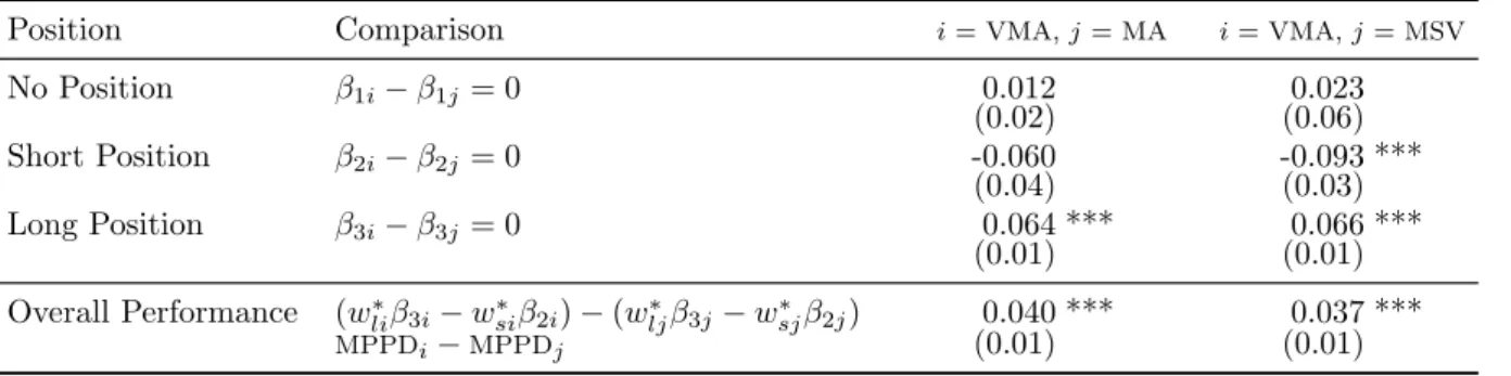
In Panel A of Table 4, we present the estimation results for the SUR mdoel along with the Newey-West (1987) robust standard errors. First of all, there is strong evidence indicating that the best VMA rule does have predictive ability for both upward and downward prcie movements, while the best MA and best MSV rule are only capable of detecting upward price movements. We also compare the mean profit per day based on signals of long position and short-position issued by the best VMA rule, the best VMA rule, and the best MSV rule. The Wald test results in Table 5 show that the mean profit the best VMA rule gains from its long positions is significantly greater than those of the others. Its mean profit over the short-position periods is significantly greater than that of the best MSV rule, while there is no significant difference in the average short-position profit between the best VMA rule and the best MA rule.

In addition to mean profits over the short-position periods and the long-position pe-riods for the three competing rules (based on the size and value of β2 and β3), we also

T able 1: The P erformance of the Best T rading Rule in the F ull Sample This table presen ts the SP A test results on the profitabilit y of 5,162 tec hnical trading rules for the p erio d b et w een Oct 1, 1928 and June 28, 2010. W e rep ort the p e rformance of the b est trading rule in eac h trading fa mi ly with their ranking in the univ erse of 5,162 rules, the n um b er of trades, daily and an n ualized Return they obtain with one-w a y transaction cost 0.05% , and their p -v alue on the SP A te st. There are tw o signals, long and short, in one trade; therefo re, the total trading n um b er of the b est VMA rule is 563 indicating tha t it has 1,126 signals. Daily return is computed from dividing the cum ulativ e return in this p erio d b y the sample size (20,526 da ys). Ann ual return is calculated b y m ultiplying the daily return b y 25 2 b ecause w e ha v e 252 tra di n g da ys p er ann um. SP A (C) is the SP A p − v alue. * denotes si g ni fican c e at the 10% lev el, **denotes significance at the 5% lev el, and *** denotes significance at the 1% lev el. Best T rading Rule in Eac h T A F amily Rank Num b er of T rades Daily Return Ann ualized Return SP A (C) VMA a 1 563 0.0325% 8.18% 0.006 *** MSV b 3 400 0.0303% 7.64% 0.020 ** MA c 7 49 0.0279% 7.04% 0.050 * FR d 11 23 0.0265% 6.67% 0.092 * CB e 141 1878 0.0198% 4.98% 0.492 SR f 988 410 0.0105% 2.64% 0.742 Note: aThe b est rule on the VMA family: α = 0 .049 (N = 40) 、 σ 15 ,n t 、 σ 30 ,r ef t 、 0.0005 band. bThe b est rule on the MSV (Momen tum Strategy in V olume) family: 2 -da y mo v ing a v erag e 、 250-da y R OC 、 0.15 o v erb ough t/o v ersold rate 、 50 fixed holding da ys. cThe b est rule on the MA family: 10-da y short-run mo ving a v erage 、 250-da y lo ng-run m o ving a v erage 、 0.001 band. dThe b est rule on the FR fa m ily: 0.05 filter rate 、 the highest and lo w est price o v er the 2 most recen t da ys. eThe b est rule on the CB famil y : the high price o v er previous 5 da ys is within 0.01 of the lo w price o v er previous 5 da ys 、 0.0005 band 、 10 fixed holding da ys. fThe b est rule on the SR famil y : the maxim um(m inim um) price o v er the previous 50 da ys b y band 0.01 、 10 fixed holding da ys. 7

T able 2: The P erformance of the Best T rading Rule in the Sub-Sample s This table rep orts the SP A test results on the profita bil it y of 5,162 tec hnical trading rules in tw o sub-sample s as a robustness chec k. The criteri o n used to create sub-samples is ba sed on Qi and W u (2006). P anel A and B demonstra te the p erf ormance of the b est trading rule in eac h trading family with one-w a y transaction cost 0 .0 5% in the first an d second sub -sample , resp ectiv ely . * deno te s significance at the 10% lev el, **denotes significance at the 5% lev el, and ** * denotes significance at the 1 % lev el. Best T rading Rule in Eac h T A F amily Rank Num b er of T rades Daily Return Ann ualized Return SP A (C) P anel A: Sub-sample 1, 1928/10/01-1969/10/28 VMA 1 870 0.0515% 12.97% 0.008 *** MSV 4 1 98 0.0430% 10.83% 0.077 * MA 13 583 0.0399% 10.06% 0.120 CB 39 933 0.0341% 8.60% 0.400 FR 138 1775 0.0294% 7.40% 0.670 SR 259 583 0.0262% 6.61% 0.848 P anel B: Sub-sample 2, 1 969/10/29-2010/06/28 VMA 1 306 0.0310% 7.82% 0.090 * MSV 2 1 41 0.0287% 7.23% 0.170 CB 4 391 0.0268% 6.75% 0.400 MA 10 108 0.0249% 6.28% 0.848 FR 25 1105 0.0237% 5.97% 0.910 SR 1169 156 0.0075% 1.89% 1 8

Table 3: The Performance of the Best Trading Rule in Other Five Sub-Samples

This table reports the performance of the best one in the universe of 5,162 technical trading rules in each sub-sample. Five sub-samples are created by the measure taken in Brock et al. (1992). The annualized return of the best rule is calculated with one-way transaction cost 0.05%. SPA (C) is the SPA p− value. * denotes significance at the 10% level, **denotes significance at the 5% level, and *** denotes significance at the 1% level.

Sub-sample the Best Rule in Each Sub-sample Annualized Return SPA (C)

Sub-sample 1 MSV 29.12% 0.428

Sub-sample 2 VMA 10.79% 0.004 ***

Sub-sample 3 VMA 13.55% 0.000 ***

Sub-sample 4 VMA 12.39% 0.186

Sub-sample 5 MSV 13.08% 0.654

compute the mean profit per day (MPPD) as follows:

MPPD_i = w_li∗β3i− w∗siβ2i, (3)

where w_li∗ and w_si∗ for each rule are the proportion of time spent on long positions and on

short positions relative to the entire sample period, respectively. Essentially, the MPPD

can be interpreted as an overall performance measure of a trading rule, which is weighted by the propostions of time spent on long positions and short positions. The results are reported in Panel B and C of Table 4. All of those three rules have significantly positive mean profit per day. Furthermore, the best VMA rule earns more than the others, as presented in Table 5.

To summarize, the fact that the best VMA can predict both upward and downward price movements, while other competing rules are only capable of detecting upward price movement give a strong evideince that higher profitability of the VMA rule might just stemg from its better forecasting ability of stock returns. In addition, the results that the time the best VMA spent in the market is the least (roughly 63.6%), while the mean profit it gains in the market is the most (see Table 5), offer another piece of evidence that the best VMA rule does enjoy a better timing in generating profitable trading signals.

5

Is the Profitability of the Trading Rule Asymmetric in Different Market

Conditions?

In the previous section, we have demonstrated a close connection between the VMA rule’s higher profitability and its better forecasting ability for stock returns. This entails two interesting questions. First, is the predictive ability of the VMA rule for future price movements sensitive to different market conditions? Second, if so, does the VMA rule still enjoy higher profitability in all market conditions?

To describe the evolution of the market condition, cyclical variations in stock returns have been widely reported (Turner et al., 1989; Hamilton and Lin, 1996; Perez-Quiros and Timmermann, 2000; Perez-Quiros and Timmermann, 2001.) Typically, bull markets and bear markets are commonly adopted to characterize equity cycles (Fabozzi and Francis, 1979; Hardouvelis and Theodossiou, 2002; Guidolin and Timmermann, 2005; Chen, 2007;

Table 4: Cumby-Modest market timing tests for the best VMA, best MA and best MSV rule

We carry out Cumby-Modest market timing tests by applying Seemingly Unrelated Regressions (SUR) as follows: 4 log P = Xiβi+ ei, i = VMA, MA, MSV,

where Xi= (z1i, z2i, z3i) and βi= (β1i, β2i, β3i)0. For each equation i, the dependent variable 4 log P , is the log return

of the DJIA (multiplied by 100). The independent variables, z1i,t, z2i,tand z3i,t, are three dummy variables. They are

set to one when the ith_{rule recommends no position, a short position, and a long position respectively; otherwise, they}

are set to zero. β1i, β2i and β3i are slope coefficients for the ithrule. We use w∗l and w ∗

s, the proportion of the time

spent long and short to the full sample period, to measure a trading rule’s overall performance, the mean profit per day (MPPD). Panel A reports the regression results for the best VMA, best MA and best MSV rule, respectively. Panel B presents their overall performances. The w∗_l and w∗s of each rule is reported in Panel C. In the parentheses are the

Newey-West (1987) robust standard errors. * denotes significance at the 10% level, ** denotes significance at the 5% level, and *** denotes significance at the 1% level.

Position Coefficient i = VMA i = MA i = MSV Panel A: Regression slopes

No Position β1i 0.020 0.008 -0.003 (0.01) (0.01) (0.06) Short Position β2i -0.117 *** -0.057 -0.023 (0.02) (0.04) (0.02) Long Position β3i 0.105 *** 0.041 *** 0.039 *** (0.01) (0.01) (0.01) Panel B: The overall trading performance

Mean profit per day (MPPDi) wli∗β3i− w∗siβ2i 0.070 *** 0.029 *** 0.033 ***

(0.01) (0.01) (0.01) Panel C: Weights adopted in theMPPDi

The time spent long/Full sample size w∗_li 0.382 0.543 0.651 The time spent short/Full sample size w∗si 0.254 0.126 0.324

The total trading time/Full sample size wi 0.636 0.669 0.975

Table 5: Comparisons in the trading performances of the best VMA, best MA and best MSV rule

This table reports comparisons between the trading performances of the best VMA rule and that of the best MA and best MSV rule. For the ith_{rule, the value of β}

2i and β3i can be interpreted as the mean profit/loss per day over its

short-position periods and long-position periods, while β1iis the average excess return when there is no signal released

by this rule. The MPPDimeasures its mean profit per day. These comparisons are implemented by the Wald test based

on the Newey-West (1987) covariance matrix. In the parentheses are the Newey-West (1987) robust standard errors. * denotes significance at the 10% level, ** denotes significance at the 5% level, and *** denotes significance at the 1% level.

Position Comparison i = VMA, j = MA i = VMA, j = MSV No Position β1i− β1j= 0 0.012 0.023 (0.02) (0.06) Short Position β2i− β2j= 0 -0.060 -0.093 *** (0.04) (0.03) Long Position β3i− β3j= 0 0.064 *** 0.066 *** (0.01) (0.01) Overall Performance (w∗_liβ3i− w∗siβ2i) − (w∗ljβ3j− wsj∗β2j) 0.040 *** 0.037 *** MPPDi−MPPDj (0.01) (0.01) 10

Table 6: Bull and bear markets in the DJIA daily price index

This table reports a summary of the bull and bear markets identified with Pagan and Sossounov (2003) algorithm over the full sample period. In the ”Days” and ”Duration” columns, we record the number of days for the whole bull and bear markets and the average days a bull or a bear market lasts.

Market Definition Number Days Duration log Return, Mean log Return, S.D. Bull Trough to peak 23 13,407 583 0.094 1.012 Bear Peak to trough 22 7,119 324 -0.124 1.397

Jansen and Tsai, 2010.) As a stylized fact, bull markets are usually associated with higher average stock returns, and a lower variance; while bear markets are associated with lower average, but a more volatile stock returns. Specifically, we are interested in investigating whether the profitability of the VMA rule in bull markets is significantly different from that in bear markets? If the profitability of the VMA rule in bear markets is significantly higher, it may imply that the information of market volatility in bear markets is more crucial for technical trading rules to forecast future price movements.

In this study, the dating algorithm proposed by Pagan and Sossounov (2003) is used to identify bull markets and bear markets in the DJIA daily index. According to Pagan and Sossounov (2003), a bull market occurs during the period when the stock price rises from a trough point and ends in a peak point; while a bear market exists during the period as the stock price moves from a peak point to a trough point. With this dating algorithm, all possible peaks and troughs in the DJIA index can be found and subsequently be used to indentify bull markets and bear markets. Table 6 presents a summary of all bull markets and bear markets so identified. There are 23 and 22 mutually exclusive and exhaustive bull markets and bear markets. We can find that, on average, durations of bull markets tend to be longer than those of bear markets in the DJIA. Specifically, Bull markets have lasted for an average of 28 months (583 days), while bear markets have lasted for 15 months (324 days). Table 6 also shows that bull markets are associated with higher but more stable stock returns while bear markets are associated with low but volatile stock returns. These results are coincident with the findings in the literature.

5.1 Market timing ability in bull and bear market

To ascertain whether the VMA rule has asymmetric, yet still dominating, performace over the equity cycles, the test of Cumby and Modest (1987) introduced in Section 4 is

applied here again with the number of independent variables for each rule Xi extended

from three to six as follows:

Xi = (z1ibl, zbl2i, z3ibl, zbr1i, zbr2i, zbr3i), i =VMA, MA, MSV, (4)

where the superscript bl and br represent bull and bear markets in the DJIA; zbl

1i, z2ibl and z3ibl

are dummy variables of the ith_{rule in bull markets, which are set to one when the i}th_rule

in bull markets recommends no position, a short position, and a long position respectively; otherwise, they are set to zero; similarly, zbr

1i, z2ibr and z3ibr are the corresponding dummy

variables for the ith _{rule in bear markets. Correspondingly, β}bl

1i, β2ibl, β3ibl, β1ibr, β2ibr and β3ibr

are the associated slope coefficients for the ith rule. If the ith rule can forecast future price increases (decreases) in all market conditions, βbl

3i and β3ibr (β2ibl and β2ibr) should

be significantly positive (negative). We also use MPPD to measure the overall trading

performance of the rule.

Table 7 reports the results of Cumby-Modest market timing tests for the best VMA, best MA and best MSV rule in bull markets and bear markets. According to the esti-mated results, the predictive ability of the best VMA rule for price movements is indeed asymmetric in bull and bear markets. It can forecast price increases in bull markets, but not in bear markets. Conversely, it is capable of detecting downward price actions in bear markets but not in bull markets. For the best MA and the best MSV rule, the asymmetry in their respective forecasting ability under different market conditions still exists, and is similar to that in the best VMA rule. Moreover, they incur losses significantly on average as they forecast price increases in bear markets and price decreases in bull markets.

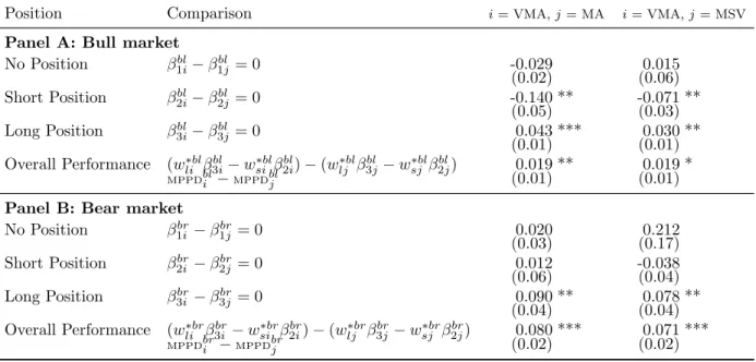
As reported in Table 8, the profitability, measured by theMPPD, of the best VMA rule in bull and bear markets are all significantly higher than those of the best MA and the best MSV rule. This answers our second question. In other words, the higher profitability of the best VMA rule is not sensitive to different market conditions. In bull markets, the mean profit from the long positions signaled by the best VMA rule is significantly higher, and the mean loss entialed from its short-position signals is significantly less than the other two trading rules. In bear markets, although there is no significant difference between the mean profit in the downward forecasting of the best VMA rule and those of the others, the best VMA rule has significant less mean loss in the upward prediction.

It is noteworthy that, in bear markets, the mean profit of the best MA rule and the best MSV rule are not significantly different from 0, while the mean profit of the best VMA rule is significantly positive. as shown in Panel B of Table 7. This offers another piece of evidence that, when asset prices change rapidly or drastically on the market, technical trading rules which do not incorporate any market volatility information cannot respond enough to the changing market conditions. Therefore, our results suggest the information of market volatility in this kind of market should be seriously considered in technical trading rules. Another interesting result in Table 9 is that the trading performance of the best VMA rule in bear markets is better than that in bull markets. As mentioned before, better profitability of the VMA rule in bear markets may imply that the device for detecting price movements, the market volatility ratio, is particularly suitable for bear markets.

6

Conclusion

In this paper, we have examined whether the information of market volatility is able to improve the predictability of technical analysis. In the previous literature, market volatility acts as a key input in many financial issues. It is, however, not clear whether market volatility has any value in technical analysis. That is, does the information of market volatility can enhance the profitability of technical trading rules? If so, why and how does it work?

We adopted the VMA rule proposed by Chande (1992) as the representative of tech-nical analysis comprising market volatility information. Market volatility in the VMA rule is built to detect does the market price make big moves in up or down direction or

Table 7: Cumby-Modest market timing tests for the best VMA, best MA and best MSV rule in bull and bear markets

The market timing test for the trading rules in bull and bear markets is carried out by Seemingly Unrelated Regressions (SUR) as follows:

4 log P = Xiβi+ ei, i = VMA, MA, MSV,

where Xi = (z1ibl, zbl2i, z3ibl, z1ibr, zbr2i, zbr3i) and βi = (β1ibl, β2ibl, β3ibl, β1ibr, β2ibr, β3ibr)0. For each equation i, the dependent

variable, 4 log P , is the log return of the DJIA (multiplied by 100). The market conditions, bull and bear markets, are represented by the index bl and br. The independent variables, zbl_1i,t, z_2i,tbl and zbl_3i,t, (z_1i,tbr , zbr_2i,tand zbr_3i,t), are dummy variables for bull (bear) markets. They are set to one when the ith_{rule in bull (bear) markets recommends no position,}

a short position, and a long position respectively; otherwise, they are set to zero. βbl

1i, β2ibland β3ibl(β1ibr, β2ibrand β3ibr)

are the associated slope coefficients for the ith_{rule in bull markets. Panel A reports the regression results and trading}

performances for these three best rules in bull markets while the corresponding results in bear markets are presented in Panel B. We use w∗_l and w∗s to measure the trading performance of the rule, the mean profit per day (MPPD). w∗bll

(w∗bls ) is defined as the proportion of the time spent long (short) to all bull periods, while wl∗br (w ∗br

s ) is the ratio

the trading rule spent for long (short) positions to all bear periods. The results are reported in Panel C on next page. In the parentheses are Newey-West (1987) robust standard errors. * denotes significance at the 10% level, ** denotes significance at the 5% level, and *** denotes significance at the 1% level.

Position Coefficient i = VMA i = MA i = MSV Panel A: Bull markets

No Position βbl_1i 0.077 *** 0.105 *** 0.062 (0.01) (0.02) (0.06) Short Position βbl_2i 0.026 0.166 *** 0.098 *** (0.03) (0.05) (0.02) Long Position βbl_3i 0.123 *** 0.080 *** 0.093 *** (0.01) (0.01) (0.01) Overall Performance w∗bl_li βbl_3i− w∗bl si β bl 2i 0.059 *** 0.040 *** 0.041 *** (MPPDbl_i ) (0.01) (0.01) (0.01) Panel B: Bear markets

No Position βbr 1i -0.078 *** -0.098 *** -0.289 * (0.02) (0.02) (0.17) Short Position βbr 2i -0.195 *** -0.207 *** -0.157 *** (0.03) (0.05) (0.03) Long Position βbr 3i -0.016 -0.107 *** -0.094 *** (0.03) (0.02) (0.02) Overall Performance w_li∗brβbr 3i − w∗brsi β2ibr 0.090 *** 0.010 0.019 (MPPDbr_i ) (0.01) (0.01) (0.02) Table 4 Continued

Measurement Weight i = VMA i = MA i = MSV Panel C: Weights adopted in measuring a technical trading rule’s performance

Bull market

The time spent long/All bull periods w∗bl_li 0.511 0.658 0.709 The time spent short/All bull periods w∗bl_si 0.138 0.077 0.261 The total trading time/All bull periods wbl

i 0.649 0.735 0.970

Bear market

The time spent long/All bear periods w∗br_li 0.141 0.327 0.544 The time spent short/All bear periods w∗brsi 0.473 0.217 0.443

The total trading time/All bear periods wbr_i 0.614 0.544 0.987

Table 8: Comparisons in the trading performances of the trading rules in each market condition

This table reports comparisons between the trading performances of the best VMA rule and that of the best MA and best MSV rule in bull and bear markets, respectively. Bull and bear markets are represented by the index bl and br. For the ith_{rule, the value of β}bl

2iand β3ibl(β2ibrand β3ibr) can be interpreted as the mean profit/loss over its short-position

periods and long-position periods in bull (bear) markets, while βbl

1i(βbr1i) is the average excess return over the no-position

periods in bull (bear) markets. MPPDbl_i (MPPDbr_i ) measures the mean profit per day the ith_{rule gains in bull (bear)}

markets. These comparisons are implemented by the Wald test based on the Newey-West (1987) covariance matrix. The Newey-West (1987) robust standard errors are in the parentheses. * denotes significance at the 10% level, ** denotes significance at the 5% level, and *** denotes significance at the 1% level.

Position Comparison i = VMA, j = MA i = VMA, j = MSV Panel A: Bull market

No Position β_1ibl− βbl 1j= 0 -0.029 0.015 (0.02) (0.06) Short Position βbl 2i− β2jbl = 0 -0.140 ** -0.071 ** (0.05) (0.03) Long Position β_3ibl− βbl 3j= 0 0.043 *** 0.030 ** (0.01) (0.01) Overall Performance (w_li∗blβbl 3i− w∗blsi β2ibl) − (wlj∗blβ bl 3j− wsj∗blβ2jbl) 0.019 ** 0.019 * MPPDbl_i −MPPDbl_j (0.01) (0.01)

Panel B: Bear market No Position βbr 1i − βbr1j= 0 0.020 0.212 (0.03) (0.17) Short Position βbr 2i − βbr2j= 0 0.012 -0.038 (0.06) (0.04) Long Position βbr 3i − βbr3j= 0 0.090 ** 0.078 ** (0.04) (0.04) Overall Performance (w_li∗brβbr 3i − w∗brsi βbr2i) − (w∗brlj β3jbr− wsj∗brβ2jbr) 0.080 *** 0.071 *** MPPDbr_i −MPPDbr_j (0.02) (0.02)

it move in a narrow range. If the market volatility does help the technical trading rules to detect market movement timelier, the VMA rule should be more profitable than other rules.

Using the Superior Predictive Ability test proposed by Hansen (2005), we found that the VMA rule outperforms others with higher profitability. Then we carry out the market timing ability test of Cumby and Modest (1987), and compare the predictive ability for upward and downward movements of the best VMA rule with that of the best MA and MSV rule. The results that the VMA rule enjoys better market timing ability may provide evidence to support the value of market volatility in better movement detecting ability.

Finally, we also investigate whether the VMA rule has differential performance in different market conditions. Empirical results suggest that in bull market, the VMA, MA and MSV rule do possess predictive ability for future upward movements, but the VMA rule earns more daily profit than the MA and MSV rule. On the other hand, the mean loss per day the VMA rule suffers is less than that of the MA and MSV rule in the downward movement forecast. In bear market, the VMA rule as well as the MA and MSV rule is able to forecast a price decrease well; however, the VMA rule has less daily loss than other rules in the upward movement forecast. As a whole, the VMA rule outperforms the MA and MSV rule both in bull and bear markets, especially the bear markets.

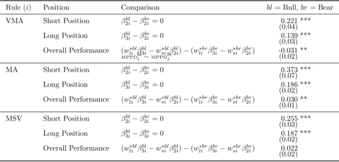
Table 9: Comparisons in the trading performances of one trading rule in different market conditions

This table reports comparisons between the trading performances of one trading rule, including the best VMA, best MA, and best MSV rule, in bull markets and that in bear markets. Bull and bear markets are represented by the index bl and br respectively. For the ith_{rule, the value of β}bl

2iand βbr2i (βbl3iand β3ibr) can be explained as the mean profit/loss

over its short-position (long-positions) periods in bull and bear markets, whileMPPDbl_i andMPPDbr_i measure its mean profit per day in these two market conditions. We use the Wald test to implement these comparisons, based on the Newey-West (1987) covariance matrix. In the parentheses are the Newey-West (1987) robust standard errors. * denotes significance at the 10% level, ** denotes significance at the 5% level, and *** denotes significance at the 1% level. Rule (i) Position Comparison bl = Bull, br = Bear VMA Short Position βbl

2i− β2ibr= 0 0.221 *** (0.04) Long Position βbl 3i− β3ibr= 0 0.139 *** (0.03) Overall Performance (w∗bl_li βbl 3i− wsi∗blβ2ibl) − (w∗brli β br 3i − w∗brsi β2ibr) -0.031 ** MPPDbl_i −MPPDbr_i (0.02) MA Short Position βbl_2i− βbr 2i = 0 0.373 *** (0.07) Long Position βbl_3i− βbr 3i = 0 0.186 *** (0.02) Overall Performance (w∗bl_li β_3ibl− w∗bl si β bl 2i) − (w∗brli β br 3i − w∗brsi β br 2i) 0.030 ** (0.01) MSV Short Position βbl_2i− βbr 2i = 0 0.255 *** (0.03) Long Position βbl_3i− βbr 3i = 0 0.187 *** (0.02) Overall Performance (w∗bl_li β_3ibl− w∗bl si β bl 2i) − (w∗brli β br 3i − w∗brsi β br 2i) 0.022 (0.02)

References

Alexander, S. S. (1961). Price movements in speculative markets: trends or random walks. Industrial Management Review 2, 7–26.

Billingsley, R. S. and D. M. Chance (1996). Benefits and limitations of diversification among commodity trading advisors. Journal of Portfolio Management 23, 65–79. Brock, W., J. Lakonishok, and B. LeBaron (1992). Simple technical trading rules and

the stochastic properties of stock returns. Journal of Finance 47, 1731–1764. Chan, L. K. C., N. Jegadeesh, and J. Lakonishok (1996). Momentum strategies. Journal

of Finance 51, 1681–1713.

Chande, T. S. (1992). Market thrust. Technical Analysis of Stocks & Commodities 10, 347–350.

Covel, M. W. (2005). Trend Following: How Great Traders Make Millions in Up or Down Markets. New York: Prentice-Hall.

Cumby, R. E. and D. M. Modest (1987). Testing for market timing ability: A framework for forecast evaluation. Journal of Financial Economics 19, 169–189.

Gehrig, T. and L. Menkhoff (2004). The use of flow analysis in foreign exchange: Ex-ploratory evidence. Journal of International Money and Finance 23, 573–594.

Hansen, P. R. (2005). A test for superior predictive ability. Journal of Business and Economic Statistics 23, 365–380.

Hsu, P. H. and C. M. Kuan (2005). Reexamining the profitability of technical analysis with data snooping checks. Journal of Financial Econometrics 3, 606–628.

LeBaron, B. (1999). Technical trading rule profitability and foreign exchange interven-tion. Journal of International Economics 49, 125–143.

Lo, A. W. and J. Hasanhodzic (2009). The Heretics of Finance: Conversations with Leading Practitioners of Technical Analysis. Bloomberg Press.

Lo, A. W., H. Mamaysky, and J. Wang (2000). Foundations of technical analysis: Computational algorithms, statistical inference, and empirical implementation. The Journal of Finance 55, 1705–1770.

Lui, Y. and D. Mole (1998). The use of fundamental and technical analysis by for-eign exchange dealers: Hong kong evidence. Journal of International Money and Finance 17, 535–545.

Neely, C. (1997). Technical analysis in the foreign exchange market: A layman’s guide. Federal Reserve Bank of Saint louis Review (Sep), 23–38.

Oberlechner, T. (2001). Importance of technical and fundamental analysis in the euro-pean foreign exchange market. International Journal of Finance and Economics 6, 81–93.

Okunev, J. and D. White (2003). Do momentum-based strategies still work in foreign currency markets? Journal of Financial and Quantitative Analysis 38, 425–447. Schulmeister, S. (2009). Profitability of technical stock trading: Has it moved from

daily to intraday data? Review of Financial Economics 18, 190–201.

Smidt, S. (1965). A test of the serial dependence of price changes in soybeans futures. Food Research Institute Studies 5, 117–136.

Sullivan, R., A. Timmermann, and H. White (1999). Data-snooping, technical trading rule performance, and the bootstrap. Journal of Finance 54, 1647–1691.

Taylor, M. P. and H. Allen (1992). The use of technical analysis in the foreign exchange market. Journal of International Money and Finance 11, 304–314.

1

國科會補助專題研究計畫項下出席國際學術會議心得報告

日期：101 年 04 月 23 日

一、參加會議經過

本次研討會我被安排在 4 月 12 日上午的 Session A.10，本場次的主題是資產定價以及槓桿 報酬 (Asset Pricing and Levered Returns)，該場次共有三位學者發表學術論文。本人發表的論 文題目為 “Levered Returns: Factors or Characteristics?”評論人 Prof. Vivek Singh 為美國密西根 大學的財金系教授，本身也是研究資產定價議題的專家。Prof. Singh 對本篇文章提供了非常多 寶貴的建議，讓本篇論文在將來投稿前，有一個良好的修正依據。

同時，本人也擔任同一場次另一篇文章 “The Role of Multifactors in Asset Pricing Models” 的評論工作，這一篇文章主要也是有關資產定價的學術論文，對於研究資產定價相關議題有 相當的幫助。

除了我自己報告跟評論的場次外，我也參加了幾場其他學者的專題演講。值得一提的是 Ippolito 等學者在 Section D.5: Leverage and Capital Structure 中所報告的 “The Relative Leverage Premium” 這一篇文章，雖然使用不同的研究方法，但與本人在這次會議發表的文章有相當的近 似性，為瞭解財務槓桿對於資產定價的影響提供了另一個思考的角度，也對於主要研究問題的釐 清有不錯的助益。

計畫編號

NSC 100-2410-H-004 -051 -

計畫名稱

探索市場波動度在技術分析中所提供的訊息

出國人員

姓名

林信助

服務機構

及職稱

國立政治大學國際貿易學系副教授

會議時間

101 年 4 月 11 日

至

101 年 4 月 14 日

會議地點

美國波士頓

會議名稱

(中文)

東部金融協會 2012 年會

(英文) Eastern Finance Association 2012 Annual Meeting

發表論文

題目

(中文) 財務槓桿報酬：因子，抑或特徵？

2

二、與會心得

這次出國參加國際學術研討會，除了從其他國家學者身上得到寶貴的建議之外，對於自己 研究議題重要性之肯定也有所助益外。另外，與其他與會學者之間的研究經驗交流，也讓我 獲益匪淺。

三、考察參觀活動(無是項活動者略)

無。

四、建議

無。

五、攜回資料名稱及內容

無。

六、其他

無。

Eastern Finance Association

2012 Annual Meetings

April 11 - 14, 2012

Hyatt Regency Boston

Boston, Massachusetts

December 1, 2011 Dear Professor Lin,

I am pleased to inform you that your paper entitled "Levered Returns: Factors or Characteristics?" has been provisionally accepted for the 2012 Eastern Finance Association (EFA) Annual Meetings at the Hyatt Regency in Boston, Massachusetts, April 11 - 14, 2012. Please notify your co-authors of this acceptance. More

information will be forthcoming regarding the time and date of your presentation. If circumstances have arisen and you now are unable to attend the conference, please let me know as soon as possible but no later than January 9, 2012. My email is efapc2012@gmail.com.

The EFA requires at least one author to register by January 9, 2012 to secure a final acceptance of the paper on the program. The reason for this requirement is to reduce the number of late cancellations by authors of

accepted papers. Graduate students: even if your co-author registers, you must register by January 9, 2012 in order for your registration fee to be waived. If you do not register by this deadline, you will be required to pay the full fee to attend the conference.

To register, please go to the EFA website http://etnpconferences.net/efa/ and click on the "Meetings

Registration" link on the right-hand side of the EFA webpage. Registration will require payment by credit card. If at least one author has not registered by January 9, 2012, your paper will be removed from the program. IMPORTANT NOTE: All presenting authors are required to discuss a paper. If you are presenting multiple papers, you should be willing to discuss as many papers as you are presenting. If you are unsure whether you will be able to fulfill this obligation, please e-mail me as soon as possible at efapc2012@gmail.com. If you have not already signed up to participate on the website, please indicate your willingness to discuss and chair sessions in the subject area(s) of your choice. Please click on the "Participate" link located on the EFA website at http://etnpconferences.net/efa/ to volunteer to serve as a discussant or session chair. The preliminary

program for the conference should be available on the EFA website by February 1, 2012, and you will be able to volunteer to chair a specific session or discuss a particular paper at that time.

Awards will be given this year for outstanding papers in a variety of areas. There will also be at least one special graduate student outstanding paper award. In order to receive an outstanding paper award, at least one of the authors must present the paper at the meetings.

The preliminary program will be posted on the EFA website by February 1, 2012. Dates and times of your sessions will be available at that time. If you have special needs regarding the time or day of your presentation or need special accommodations please email me at efapc2012@gmail.com so that I can take them into consideration in preparing the preliminary program. I look forward to seeing you at the EFA Annual Meetings at the Hyatt Regency in Boston, Massachusetts, April 11 - 14, 2012.

Congratulations,

來源: no-reply@etnpconferences.net <no-reply@etnpconferences.net> 收信: shjlin@nccu.edu.tw

日期: Thu, 1 Dec 2011 17:16:27 -0600

Beverly

Beverly B. Marshall

Eastern Finance Association VP-Program Auburn University

e-mail: efapc2012@gmail.com

Levered Returns: Factors or Characteristics?

∗

Kuan-Cheng Ko

Department of Banking and Finance

National Chi Nan University

Shinn-Juh Lin

Department of International Business

National Chengchi University

Ju-Fang Yen

Department of Finance

National Taiwan University

February 2012

Abstract

This paper investigates whether the leverage anomalies are better explained by the risk-based factor model or the characteristic-based model. Following Daniel and Titman’s (1997) methodology, we show that Ferguson and Shockley’s (2003) three-factor model has not only offered a risk-based explanation for the leverage-return relations documented in the literature, but also explained the book-to-market (BM) effect and reconciled findings in this paper with those in Daniel and Titman (1997). The support for Ferguson and Shockley’s (2003) three-factor model is even stronger for the pre-1980 period. Finally, empirical results based on other G7 countries further support Ferguson and Shockley’s (2003) model in explaining the leverage anomalies.

JEL Classification: G10; G12; G32.

Keywords: characteristic model; factor model; leverage puzzle.

∗_{We appreciate the helpful comments and suggestions from Pin-Huang Chou, Tunde Kovacs,} Ji-Chai Lin, and conference participants at the 20th European Financial Management Association Con-ference in Portugal, as well as seminar participants at National Chi Nan University and National Dong Hua University. Corresponding author: Kuan-Cheng Ko. Email: kcko@ncnu.edu.tw; Address: No. 1, University Rd., Puli, 54561 Taiwan; Tel: 886-49-6003100 ext. 4695; Fax: 886-49-2914511. Ko acknowledges financial support from the National Science Council of Taiwan (Grant number 99-2410-H-260-030). Lin acknowledges financial support from the National Science Council of Taiwan (Grant number 100-2410-H-004-051).

1

Introduction

One of the famous propositions in modern corporate finance is the leverage-return rela-tion proposed by Modigliani and Miller (1958), who argue that expected stock returns should increase with financial leverage. However, empirical evidence on the leverage-return relation is mixed, and is further complicated with two different definitions of financial leverage, namely book-leverage and market-leverage. For example, Bhandari (1988) demonstrates the existence of a positive premium for stocks with a high market-leverage. Fama and French (1992), instead, find that stock returns are related to both book-leverage and market-leverage, but with opposite signs. They further show that the book-to-market (BM) ratio, as the combination of two leverage variables, plays the dominant role in explaining stock returns.

An alternative interpretation of the evidence is that markets are efficient, and there exists some risk factors that capture the leverage risk. In a multi-factor framework a la Ross’s (1976) arbitrage pricing theory (APT), Fama and French (1993) construct two mimicking portfolios formed on size (i.e., SMB) and BM (i.e., HML) as common risk factors to capture variations in stock returns. Fama and French (1993, 1995, 1996, 1998) demonstrated that the SMB and HML factors are priced in both the U.S. and inter-national stock markets. However, Daniel and Titman (1997) propose a characteristic-based model and argue that Fama and French’s (1993) three-factor model still fails to fully account for the cross-sectional regularities related to size and BM. They therefore conclude that it is firms’ characteristics rather than risks that drive the BM premium. In addition to numerous empirical explorations on the asset-pricing regularities, it is also argued that such leverage premia might be related to rational asset pricing factors. For example, Ferguson and Shockley (2003) construct two factors to capture the part of returns associated with relative leverage (based on the ratio of market debt-to-equity,

D/E) and the part of returns associated with relative distress (based on the Altman’s Z-score), and show that the two proposed factors subsume Fama and French’s SMB and HML factors in explaining the cross-sectional variation in stock returns on the 25 portfolios formed on size and BM ratio. Ferguson and Shockley (2003) also demonstrate that the mis-estimated beta increases with the firm’s leverage, which seems to imply that leverage-related variables could possibly capture mis-estimated beta risk. Nevertheless, leverage as one of firm’s many characteristics could also convey information independent of the covariance structure of stock returns that helps explain expected stock returns.

The main thrust of this paper is to ascertain whether the leverage-return relation demonstrated in Ferguson and Shockley (2003) is truly arising out of some factor struc-ture, or whether it is due to the documented “leverage anomaly”. To address this important question, we apply the methodology developed by Daniel and Titman (1997) to examine whether Ferguson and Shockley’s (2003) model is really picking up some

mis-measured market risk.1_{Within this framework, we can discuss whether driving forces}

behind the leverage anomalies are more risk-based or more behavioral-based. Specifi-cally, we examine whether book-leverage and market-leverage, as separate effects, are better explained by Ferguson and Shockley’s (2003) leverage-based asset-pricing model. Furthermore, since Fama and French (1992) find that the explanatory power of the two leverage variables in combination is characterized by a firm’s BM, we also exam-ine whether leverages and BM are driven by the same forces. Taking into account that Fama and French’s (1993) three-factor model is rejected by the BM-based charac-teristic model (Daniel and Titman, 1997), we extend our test to examine the relative explanatory power of Ferguson and Shockley’s (2003) model against the BM-based char-acteristic model. Such an investigation is helpful in ascertaining whether Daniel and Titman’s (1997) finding is due to misspecification of the assumed Fama and French’s 1_{Other applications and extensions of this method include Davis, Fama, and French (2000), Daniel,}

Titman, and Wei (2001), Gebhardt, Hvidkjaer, and Swaminathan (2005).

(1993) asset-pricing model.

By studying a sample of of all NYSE/AMEX/NASDAQ ordinary common stocks from July 1964 to December 2008, we show that Ferguson and Shockley’s (2003) three-factor model has not only offered a risk-based explanation for the leverage-return re-lations documented in the literature, but also explained the BM effect and reconciled findings in this paper with those in Daniel and Titman (1997). These findings sup-port the factor-explanation to the leverage-return relation, and confirm Ferguson and Shockley’s (2003) argument that size and BM, as proxies for firm leverage and dis-tress, are explained by their leverage-based factor model. Subperiod analysis further demonstrates that the support for Ferguson and Shockley’s (2003) three-factor model is most pronounced for the pre-1980 period. Finally, empirical investigation based on an independent sample from other non-U.S. G7 countries further supports Ferguson and Shockley’s (2003) model in explaining the leverage anomalies, suggesting our results are free from the data-snooping bias proposed by Lo and Mackinlay (1990).

The rest of the paper is organized as follows. Section 2 describes data used in this paper, establishes the leverage-return relation, and examines its connection with the BM effect. In Section 3, we lays out methodologies in testing whether the driving forces of leverage premia are more risk-based or characteristics-based, and present empirical results for characteristic-balanced portfolios sorted by both book-leverage and market-leverage portfolios, with robustness checks through subperiod analysis, and considera-tion of January seasonality. In Secconsidera-tion 4, we examine whether Ferguson and Shockley’s (2003) model can also explain the BM effect, and reconcile findings in this paper with those in Daniel and Titman (1997). Further examinations conducted based on other G7 countries as a robustness check is provided in Section 5. The last section concludes this paper.

2

Data and the Leverage Premia

2.1

Data Description

Our sample consists of all NYSE/AMEX/NASDAQ ordinary common stocks from July 1964 to December 2008. We obtain monthly data on returns and market equity from the Center for Research in Security Prices (CRSP) database. Book equity and debt data are retrieved from the Compustat. Following Fama and French (1992), for the period from July of year t to June of t + 1, we use a firm’s market equity at the end of June of year t as its size, and together with the book equity at the end of December

of year t− 1 to construct the book-to-market ratio. Book-leverage is calculated as the

ratio of book value of debt to total assets, while market-leverage is calculated as the ratio of book value of debt to the sum of market equity and book value of debt at the

end of December of year t− 1. To be included in our sample, we require a firm to

have at least 24 monthly returns between January of year t− 5 and December of year

t− 1 to calculate the ex ante factor loadings for individual stocks. As in Fama and

French (1992), we exclude financial firms and stocks with negative book equity from our sample.

To calculate Ferguson and Shockley’s (2003) D/E and Z factors (denoted as RD/E

and RZ), we retrieve the required accounting variables from the Compustat. The two

factors are constructed over the period from July 1964 to December 2008. The detail of the portfolio formation process is presented in the Appendix.

2.2

Do Leverage Premia Exist?

Based on the data constructed in Section 2.1, we examine whether stock returns are related to firm leverage. More specifically, we examine whether there exist significant

premia for book-leverage and market-leverage, respectively. To do so, we construct characteristic-sorted portfolios by following a procedure similar to the one used by Fama and French (1992). From July of year t to June of year t+1, individual stocks are sorted into five quintile portfolios according to their corresponding market-leverage (or

book-leverage) at the end of December of year t− 1. The breakpoints are determined using

all NYSE firms in the sample. From July of year t to June of year t + 1, we calculate the equally-weighted monthly returns on these portfolios. The portfolios are rebalanced once a year in June.

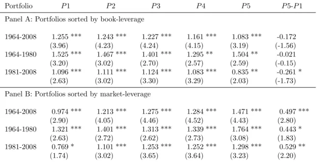
[Insert Table 1 about here]

Panel A of Table 1 presents average monthly returns for book-leverage sorted portfo-lios, and return spreads between the most-levered quintile portfolio and the least-levered quintile portfolio (P 5-P 1) for the full period, and two subperiods before and after 1980. The cutoff point is chosen because George and Hwang (2010) find that the book-leverage premium is is only significantly different from zero in the post-1980 period. Consistent with George and Hwang (2010), our reported premia for high minus low book-leverage are 0.172% (with a tstatistic of 1.56), 0.021% (with a tstatistic of 0.15), and -0.261% (with a t-statistic of -1.73) for 1964-2008, 1964-1980, and 1981-2008 periods, respectively. Panel B of Table 1 reports results for market-leverage-sorted portfolios Unlike book-leverage premia, market-leverage premia for the full sample and two sub-periods are all significant. The P 5-P 1 spreads are 0.497 (with a t-statistic of 2.80), 0.443 (with a t-statistic of 1.83), and 0.529 (with a t-statistic of 2.20), respectively.

Thus, we confirm the existence of both book-leverage premia and market-leverage premia in our sample. Among which, the negative relationship between book-leverage and stock returns holds only for the post-1980 period.

2.3

Are Leverage Effects Independent of the Book-to-Market

Effect?

Although there exist both book-leverage and market-leverage premia in our sample, Fama and French (1992) argue that the BM captures both book-leverage and market-leverage anomalies in the Fama-MacBeth cross-sectional regression. They observe sim-ilar slopes in absolute values but with opposite signs for book-leverage and market-leverage variables. Furthermore, they show that the BM slope is close in absolute value to both slopes for the two leverage variables, and conclude that the combination of book-leverage effect and market-leverage effect is an equivalent way to interpret the BM effect in stock returns.

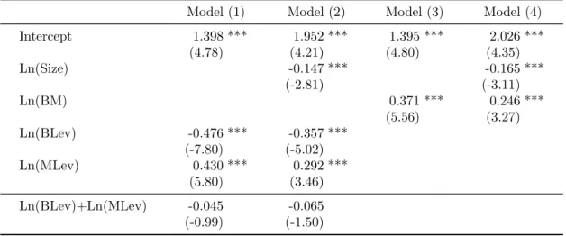
To further clarify the relation between leverage effects and the BM effect, we examine whether Fama and French’s (1992) argument holds true in our sample. Similar to Fama and French (1992), we take logarithm form for all explanatory variables. Slightly different from Fama and French (1992), we use the debt-to-equity ratios, instead of the asset-to-equity ratios, as the leverage variables.2

[Insert Table 2 about here]

As reported in Model (1) of Table 2, the coefficients on the natural logarithm of the leverage variables, Ln(BLev) and Ln(MLev), are -0.476 (t-statistic = -7.80) and 0.430 (t-statistic = 5.80), respectively. An additional test on Ln(BLev)+Ln(MLev) is also provided in the bottom row of Table 2. Conceptually, if BM captures the informational content of both book-leverage and market-leverage, the sum of the coefficients on the two leverage variables should not be significantly different from zero. The insignificant value of -0.045 (t-statistic = -0.99) confirms such a conjecture. As presented in Model 2_{We obtain similar results by using asset-to-equity ratios as proxies for leverage, as employed by}

Fama and French (1992).

(2), the results are largely the same when firm size, Ln(Size), is included in the regres-sion, where the test statistic on Ln(BLev)+Ln(MLev) is -0.065 (t-statistic = -1.50). Moreover, coefficients on BM reported in Models (3) and (4) are both significant, and are quantitatively similar to the absolute values of the coefficients on the two leverage variables.

Overall, we have documented two stylized facts. First, we find that stock returns are related to both book-leverage and market-leverage in our data. Second, the two leverage effects in combination is not independent of the BM effect, suggesting that they are not new anomalies beyond the BM effect. However, an intriguing question remains as to what driving forces are behind the leverage effects, risk-based or behavioral-based? And, if there is a common force that drives both leverage effects, does it also explain the BM anomaly? We offer more detailed discussions of these questions in Section 3 and Section 4.

3

The Leverage Premia: Factors or Characteristics?

3.1

Construction of Test Portfolios and Testing Hypotheses

In this section, our objective is to investigate whether the leverage premium is better described by a risk-based or a characteristic-based argument. To that end, we employ the leverage-based three-factor model of Ferguson and Shockley (2003), which implies the following risk-return relation:

E(Ri)− Rf = biRM kt+ diRD/E+ ziRZ. (1)

One way to test Equation (1) is to test the joint-zero-intercept hypothesis of the fol-lowing regression model:

Ri,t− Rf,t = ai+ biRM KT,t+ diRD/E,t+ ziRZ,t+ εi,t. (2)

According to the leverage-factor-based argument, the intercepts, ais, should be zero for

all stocks. On the contrary, the characteristic-based argument says that non-zero ais are

expected when stocks’ factor loadings on RD/E do not line up with firms’ characteristics.

If a firm’s leverage is correlated with its RD/E loading, it is not obvious whether it

is the factor model or the characteristic model that better explains stock returns. To distinguish the factor model from the characteristic model, we follow Daniel and Titman (1997) in forming portfolios by isolating variations in factor loadings so that they are independent of firm characteristics. To do so, we first sort individual stocks in an independent two-way sorting into three book (or market) leverage groups and three firm-characteristics (using size or Z-score) groups at the end of June of each year, where the breakpoints are the 33rd and 67th percentiles for the NYSE firms in the sample. This results in nine different characteristic portfolios.

We then allocate individual stocks within each of the nine portfolios into five

sub-portfolios using pre-formation RD/E slopes (di), which are obtained from estimating

Equation (2) with monthly returns of the past five years (with the availability of data for at least 24 observations) ending in December of year t− 1.3 _{After sorting individual}

stocks into five factor-loading portfolios within each of the nine characteristic portfolios, we calculate the value-weighted returns for each of the 45 test portfolios from July of year t to June of year t + 1. Consequently, nine characteristic-balanced portfolios, denoted

3_{To have better predictions of the future covariance of firms with the factors, we follow Daniel}

and Titman (1997) in using the constant-weight factor-portfolio returns to construct the pre-formation factor loadings. That is, we apply the portfolio weights of factor portfolios (RD/E and RZ) at the end of June of year t to the individual stock returns from December of year t− 1 to January of year t− 5, and calculate returns on the constant-weight factor portfolios in estimating the pre-formation di slopes.

as (Hh− Lh)i, i = 1, . . . , 9, are constructed by investing a one-dollar long position in

the high (fourth and fifth) di portfolios, and a one-dollar short position in the low (first

and second) di portfolios within each of the nine characteristic-sorted groupings. If the

characteristic model is correct, time-series average returns of characteristic-balanced portfolios should be insignificantly different from zero, since they hold long and short positions of stocks with similar characteristics. By contrast, time-series average returns will be positive if the leverage-based factor model is true, because the

characteristic-balanced portfolios have high loadings on the RD/E factor.

As in Daniel and Titman (1997), we propose an alterative test of the factor model against the characteristic model, which can be inferred from the estimated intercept terms in the following regressions:

(Hh− Lh)i,t = ai+ biRM KT ,t+ diRD/E,t+ ziRZ,t+ εi,t, for i = 1, . . . , 9. (3)

The null hypothesis in favor of the factor model predicts that the intercepts from Equa-tion (3) are insignificantly different from zero. By contrast, the alternative hypothesis in favor of the characteristic model predicts negative intercept terms in Equation (3), because the positive di loadings for the (Hh−Lh)i portfolios do not affect the expected

returns of the characteristic-balanced portfolios.

As a joint test, we also construct an equally-weighted portfolio, denoted as (Hh−

Lh)p, out of the nine characteristic-balanced portfolios, (Hh− Lh)is. The model

spec-ification now becomes:

(Hh− Lh)p,t= ap+ bpRM KT ,t+ dpRD/E,t+ zpRZ,t+ εp,t. (4)

The null hypothesis in favor of the factor model of the joint test predicts that ap

is insignificantly different from zero. By contrast, ap should be negative under the