國 立 交 通 大 學
工學院精密與自動化工程學程
碩 士 論 文
以循圓測試法建立 HexGlider 型平行機構之運動誤差模型
與診斷方法
Modeling and Diagnosis of Motion Error of a HexGlider
Manipulator Based on a Circular Test Method
研 究 生 : 陳 裕 都
指導教授 : 成 維 華 博士
以循圓測試法建立 HexGlider 型平行機構之運動誤差模型與診斷
方法
Modeling and Diagnosis of Motion Error of a HexGlider Manipulator
Based on a Circular Test Method
研 究 生: 陳 裕 都 Student : Yu-Du Chen
指導教授: 成 維 華 博士 Advisor : Dr. Wei-Hua Chieng
國 立 交 通 大 學 工學院精密與自動化工程學程
碩 士 論 文
A Thesis
Submitted to Degree Program of Automation and Precision Engineering College of Engineering
National Chiao Tung University in Partial Fulfillment of the Requirements
for the Degree of Master of Science
In
Automation and Precision Engineering July 2006
Hsinchu, Taiwan, Republic of China
以循圓測試法建立 HexGlider 型平行機構之運動誤差模型與
診斷方法
學生:陳裕都 指導教授:成維華 博士 國立交通大學精密與自動化工程學程碩士班 摘 要 本論文主要研究的範疇與目的,係針對 Hexglider 構型之平行機構的 運動誤差,建立其數學模型與診斷方法。 首先,對於所欲研究之平行機構,建立其導致運動誤差的幾何誤差源 模型。除了推導該種構型平行機構的驅動滑塊與輸出平台之間運動轉換的 關係,同時分析出可能導致其發生運動誤差的幾何誤差源與相關之參數誤 差,並利用於運動轉換關係所得到的結果,建構個別誤差源之誤差模型, 以瞭解各誤差源在理論上對於該機構之運動精度所造成的影響。 更進一步,以實驗的方式,對此待測之平行機構,進行實機之雙球桿 循圓測試,來作誤差診斷。其主要目標,在於找出該機構可能存在之幾何 誤差源,並且診斷各誤差源之參數誤差的大小。 在數學上,本論文將利用最小平方法原理,將整個平行機構綜合誤差 經循圓測試所量得軌跡,解構為由個別誤差源所對應之循圓運動軌跡的合 成,並將針對個別誤差之參數誤差進行估測,以實現該機構之誤差診斷, 適當地發展出該機構運動誤差的校驗方法。換言之,只要運用雙球桿量測 裝置,正確地對待測之平行機構,量得循圓運動軌跡,即可有效地分析出 該機構之各項幾何誤差源,並且診斷其誤差參數之大小。如此,不論是對 於該種平行機構之機械本體的精度的改善,或者是終端輸出的位置誤差的 補償,都將會有莫大的助益。Modeling and Diagnosis of Motion Error of a HexGlider
Manipulator Based on a Circular Test Method
Student:Yu-Du Chen Advisors:Dr. Wei-Hua Chieng
Institute of Automation and Precision Engineering National Chiao Tung University
Abstract
This thesis is mainly focused on the study of analyzing and identifying specified motion errors for the hexglider type of parallel manipulator.
First, the investigated geometric errors resulting in motion errors for the target parallel manipulator are to be modeled. We begin at deriving the kinematic transformation relationships between the sliders and the end effector of the parallel manipulator. Geometric resources of motional deviations, including translate and angular ones, resulting from the manufacturing or assembly of guideways and linkages are classified and modeled with the analytical results of the kinematics.
Next, the double ball bar test is experimentally applied to the desired parallel manipulator for the study of the error diagnosis. We aim to identify geometric errors existing at the manipulator from the measured data.
Mathematically, the least square method is adopted in the thesis to the identification of geometric errors. The circular contour of the overall error of the parallel mechanism obtained from the double ball bar test will be fitted by theoretic deviations caused by error sources, and their parameter errors are to be estimated.
Based on the results, we will propose a measurement method and evaluating procedure to identify geometric deviations. It can be utilized as a calibration method of the hexglider manipulator. In other words, provided that the double ball bar test is applied to the desired parallel manipulator correctly, geometric deviations existing at the manipulator can be identified. Thus, it will significantly benefit to either the compensation of the position and orientation errors or the improvement of the mechanism accuracy for the hexglider type of parallel manipulator.
誌 謝
本論文之完成,首先要感謝指導較授 成維華博士,在我碩士班的求學 期間,諄諄教誨,循循善誘,不論是在理論或實驗上,皆不厭其煩地給予 諸多的指導與啟發,令我在學問的追求與學理的研究上,除了累積豐富的 知識與難得的經驗,同時也獲得相當程度的成長。 感謝所有口試委員深刻且獨到的指教,由於您們寶貴的意見,使得本 論文更具可讀性。 在出社會工作多年之後,選擇重回學校讀書研究,父母的認同與支持 ,給了我極大的勇氣與信心;他們多年來無微不至的教養與提攜,黑髮換 白髮,成就了今日的我。謹以獲得此一學位的榮耀,獻給最摯愛的雙親。 特別感謝博士班游武璋學長關於機構誤差理論的推導,楊家豐學長在 最小平方法應用上的討論,還有童永成學長與吳炳霖同學在實驗上的鼎力 協助,同時也要感謝交通大學機研所智慧機電實驗室提供模擬器平台。有 了大家的幫忙,克服了每個過程中所遭遇的種種困難,使得整個論文的研 究工作,得以順利地完成。 最後,對於所有家人以及關心我的友人,由衷地感謝您們在這段日子 裏,持續不斷地對我的關懷與鼓勵。Contents
摘 要 i Abstract ii 誌 謝 iii Content iv List of Figures viList of Tables viii
Chapter 1 Introduction 1
1.1 Parallel manipulator 1
1.2 Motion Errors 2
1.3 Literature Review 4
Chapter 2 Kinematics Transformation 10
2.1 SP-120 Hexglider Manipulator 10
2.2 Inverse Kinematics 11
2.3 Kinematics of RSSR Mechanisms 16
2.4 Newton-Raphson Method 17
2.5 Forward Kinematics 21
Chapter 3 Modeling of Motion Errors 24
3.1 Introduction 24
3.2 Error Descriptions 24
3.3 Error Modeling 26
3.4 Error Diagnosis 35
Chapter 4 Measurement of Motion Errors 37
4.1 Double Ball Bar Measurement Device 37
4.3 Experimental Results 39
Chapter 5 Least Squares Estimation 41
5.1 Error Estimation 41
5.2 Least Square Method 42
5.3 Simulation and Diagnosis 44
5.4 Discussion 45
Chapter 6 Conclusion 48
List of Figures
Figure 1.1 Outline of this Study 53
Figure 1.2 Prototype of SP-120 54
Figure 2.1 Hexglider parallel manipulator 55
Figure 2.2 Geometric relationships with respect to the mobile plate 55 and the fixed plate
Figure 2.3 Geometric relationships with respect to the two linkages 56 and two sliders on a guideway
Figure 2.4 RSSR mechanism 56
Figure 2.5 Forward kinematics of the hexglider manipulator under 57 investigation
Figure 3.1 Geometric error sources of a hexglider manipulator 57
Figure 3.2 (a) Guideway translation error 58
Figure 3.2 (b) Guideway rotation error I 58
Figure 3.2 (c) Guideway rotation error II 58
Figure 3.3 Guideway translation error along X-axis for RSSR 59 mechanism╴Type I
Figure 3.4 Guideway translation error along X-axis for RSSR 59 mechanism╴Type II
Figure 3.5 Guideway translation error along Y-axis for RSSR 60 mechanism╴Type I
Figure 3.6 Guideway translation error along Y-axis for RSSR 60
mechanism_Type II
Figure 3.7 Guideway translation error along Z-axis for RSSR 61 Mechanism╴Type I
Figure 3.8 Guideway translation error along Z-axis for RSSR 61 Mechanism╴Type II
mechanism_Type I
Figure 3.10 Guide way rotation error on XY plane for RSSR 62 mechanism_Type II
Figure 3.11 Guide way rotation error on YZ plane for RSSR 63 mechanism_Type I
Figure 3.12 Guide way rotation error on YZ plane for RSSR 63 mechanism_Type II
Figure 3.13 Guide way rotation error about the center of the base for 64
RSSR mechanism__Type I
Figure 3.14 Guide way rotation error about the center of the base for 64
RSSR mechanism__Type II
Figure 3.15 Procedures of modeling the overall profile error 65 Figure 3.16 Error simulation (1)_linkage length error (δ=0.01mm) 66 Figure 3.17 Error simulation (2) _slides positioning error (δ=0.01mm) 67 Figure 3.18 Error simulation (3) _guideway assembly error 68
(δ=0.01mm)
Figure 3.19 Error simulation (4)_guideway rotation error (ε=0.01deg ) 69 Figure 3.20 Error simulation (5)_guideway rotation error (ε=0.01deg) 70 Figure 4.1 Configuration of the error diagnosis experiment 71
Figure 4.2 Double ball bar system 72
Figure 4.3 Procedures of DBB test & error diagnosis 73 Figure 4.4 Procedures of the setup and data capture of the DBB test 74 Figure 4.5 Design of the auxiliary fixture for DBB test 75 Figure 4.6 Testing path of the circular contour tracking 75 Figure 4.7 The completed setup of the DBB system 76 Figure 4.8 Polar plot obtained from the data capture of DBB test 76 Figure 5.1 Procedures of curve fitting with least square estimation 77
List of Table
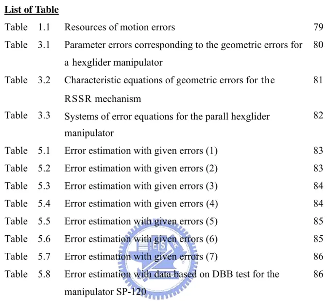
Table 1.1 Resources of motion errors 79
Table 3.1 Parameter errors corresponding to the geometric errors for 80
a hexglider manipulator
Table 3.2 Characteristic equations of geometric errors for the 81 RSSR mechanism
Table 3.3 Systems of error equations for the parall hexglider 82 manipulator
Table 5.1 Error estimation with given errors (1) 83 Table 5.2 Error estimation with given errors (2) 83 Table 5.3 Error estimation with given errors (3) 84 Table 5.4 Error estimation with given errors (4) 84 Table 5.5 Error estimation with given errors (5) 85 Table 5.6 Error estimation with given errors (6) 85 Table 5.7 Error estimation with given errors (7) 86 Table 5.8 Error estimation with data based on DBB test for the 86
Cahpter 1
Introduction
§1-1
Parallel ManipulatorParallel manipulators have reecently attracted increasing attentions for many applications. Numerous researchs and development effforts were devoted on them. It is well known that most industrial robots are open-chain mechanisms constructed of consecutive links connected by rotational or prismatic one degree of freedom. These serial manipulators have large workspace, high dexterity and good maneuverapility. However, they exhibit low stiffness and poor positioning accuracy due to their serial structure. As a result, their applications that require large load (e.g. machining) and high accuracy are limited.
The parallel manipulator, the end effector is attached to a movable plate which is supported in–parallel by a number of actuated links, is anticipated to possess the following advantages compared with serial manipulators : 1) High force / torque capacity since the load is distributed to several in-parallel actuators ; 2) High structural ridigity ; and 3) Better accuracy due to less cumulative joint errors.
For the high accuracy motion control of the parallel kinematic feed drive system, it is cruitial to accurately calibrate various errors of kinematic parameters such as the reference length of the strut or the location of the slide
joint. In practice, the knowledge of these identified errors is beneficial to improving the position and orientation accuracy of a parallel manipulator.
In our study, we will develope a diagnostic method for identifying kinematic parameter errors based on the DBB test, which have been widely accepted by machine tool manufactures as a standard tool to measure the contouring accuracy and diagnose error sources for conventional multi-axis machine tools. Figure 1.1 outlines the main structure of this thesis. A hexglider type of parallel manipulator developed by the intelligent mech-electric labroatory in NCTU, named SP-120 as shown in Figure 1.2, is utilized as an experimental manipulator throughout this study.
§1-2
MotionErrors
Motion errors are defined as the difference between the real and measured position and orientation of the end effector. These errors cause a deterioration of the machine performace, which in turn directly influences the final product specifications. In order to maintain high quality of performace, these errors have to be detected and eliminated.
The kinematic precision is an important item to evaulate the performance of a machine / manipulator. From the point view of kinematic precision, it means that the precision in position, velocity, and acceleration of a machine
during normal operations[1]. For a drive system with ball screws and guideways, the manufacturing error of the machine parts, the feed motion error, and the command error may have an fatal influence on the point-to-point precision of the machining workpiece or the contouring precision of the end-effector.
One of the significant requirements for the kinematic precision is to generate the movement in differert axes of a machine so that the end effector can position and orientate precisively. The contouring precision of the end-effector, a kind of the positional precision, is the accuracy of the overall system or the contour error of the system. This is defined as the actual difference in distance between the programmed path and the actual path. The contouring error is the synthetic performance of several kinds of error sources. For a machine with the drive systems of ball screws and guideways, error sources can be categorized into groups such as the position error, the feed motion error, and the command error, as illustrated in Table 1.1.[2]
Geometric errors of a manipulator are resulted from not only the manufacturing process but also the improper assembly. They include the length error of the linkage, the elastic deformation of each guideway, and the symmetric angular and positional errors of the guideways. Compared with the other errors, geometric errors are more stable and controlled easier.
Sp-120 is a parallel manipulator with the drive systems of ball screws and guideways. The improper assembly of guideways fixed on the stationary plate will have a great influence on the incorrect pose (position and orientation) of the end effector. Thus, the present study for the errors of the parallel manipulator will focus on modeling and identifying geometric errors, such as the reference length error of the strut, the location error of the slide joint, or the angular and positional deviations of guideways for the hexglider type of parallel manipulator.
§1-3 Literature Review
It is very important for manufacturing a high precisive machine to evaulate its performaces, such as accuraccy, functions,…, etc. In view of evaulating the accuracy of a machine, proper measuring tools and correct diagnostic methods are indispensable.
Measuring tools can retrieve useful calibrating data to be analyzed from a manipulator. To evaluate a machine, one must first determine what errors to be identified so as to select a suitable measureing tool. Nowadays, there are a few measuring tools available for measuring motional errors. Coordinate Measurement Machines (CMM) can detect the spatial coordinate location of a selected contact point. Laser interfermeters is ideal for measuring straightness and point-to point precision. The double ball bar (DBB) measurement systems
[3] specified in ISO 230-1 [4] as a measuring instrument has been mainly used for the circular motion tests of the conventional 3-axis machining center, and the instrument has contributed to the performance test or periodic maintenance of the machining center.
To identify errors is the major goal of implementing measurement. Two approaches, direct error identification method and indirect error identification method, are normally applied to the error identification.
The direct error identification method is performed by measuring the individual error sources directly. For example, the laser interferometer, for a translational slide, can measure six motional errors associated with a prismatic joint at different positions of moving axes of the machine in one measurement. The indirect error identification method is the way to realize the errors of the machine by means of measuring the errors of a part profile or the overall errors of machines. Mou, Donmez and Centikunt [5] used a feature-based comparison method to correlate the dimensional and form errors of a manufactured part. Inverse kinematic methods and ststistical methods were applied to estimate the contribution of the individual error component to imperfect part features.
The Double ball bar (DBB) test is another significiant example. In this method, the kinematic error of the circular interpolation of a machine is read by using a LVDT scale, and then is transmitted to a computer to be processed futhermore. Based on the error models and the principles of statistics, not only
individual errors existing at the mechanism can be identified, but what proportion of the overall noncircularity error which can be attributed to the identified error can be estimated as well.
In addition, the DBB is frequently used to measure the dynamic errors such as gain mismach, lost motion and stick-slip. All possible error sources of NC machine tools, for example, based on the motion error contour can be diagnosed.
Bryan [6] proposed that the double ball bar (DBB) measurement system is an error diagnosis method for measuring geometric errors and dynamic characteristics. Knapp [7] studied on the relationship between the contouring error and the motion error sources. Kunzman [8] and Kakino [9] described motion errors based on DBB with the characteristic matrix and the error vector respectively. S.L.Jeng et al. [10] presented a linear model (1st order approximation) and a nonlinear model (2nd order approximation) to describe the motion error due to a faulty guide way system for the multi-axis machine. M.Tsutsumi et al. [11] presented an algorithm for identifying particular deviations such as angular deviations around linear axes relating to rotary axes in 5-axeis machining center based on the DBB method.
Many publications dealt with the kinematics of Stewart platform-based manipulators have appeared since the Stewart platform was proposed by Stewart in 1965 [12]. In [13] , the kinematic behavior of a three-link, three degree-of-freedom (DOF) platform was investigated. In [14], the kinematic behavior of a 6-DOF Steward platform was studied.
The forward kinematic problem of the parallel manipulator involves systems of highly non-linear equations. Many of these studies was established on the basis of a simplified structure to reduce the nonlinearity of the equations, such that an analytical approach can be performed to complete a solution set. Important results are presented in [15] proving that the solution for spatial structures of the 3-3 type is a polynomial equation of the 16th degree, while the solution in case of 6-6 system is a polynomial equation of the 40th order [16] (there may exist up to 64 solutions which make this an impossible approach to use practically.). There also exist numerical methods that can be used to compute all of the forward kinematic solutions of parallel manipulators that have a more general configurations. These methods relied on the numerical continuation method or exhaustive mono-dimensional-search algorithm to solve the polynomial form of the loop closure equations[17 ][18 ].
Several papers discussed the accuracy analysis of a parallel manipulator and developed error models. Wang and Masory [19] investigated how manufacturing errors affect the accuracy of a Steward platform. Ropponen and Arai [20] presented an error model based on differentiation of the kinematics. Wang and Ehmann [21] developed error models for the Steward platform using differential leg length changes. K.C.Fan et al. [22] dealt with the verification of two error modeling methods, namely linkage kinematic error analysis method and the differential vector method, for the parallel machine tool structure. Although each model follows slightly different formulation, they are all able to
take errors in kinematic errors and calculate the resulting pose error. Some also calculate error sensitivities and present automated error analysis simulations.
A few authors have also presented calibration algorithms for the Stewart platform. Zhuang and Roth [23] developed a calibration method that holds one leg length fixed while varing the others, allowing the kinematic parameters of each leg to be indentified individually while redundant parameters are limited. Wampler et al. [24] developed a slightly different type of calibration based on imlplicit loops. A method to use redundant sensors on passive joints to calibrate parallel manipulators was formulated by Zhuang and Liu [25]. K.F.Ehmann et al. [26] presented a calibration method using a ball bar or other simple length measuring device to act as an ‘extra leg’ for the calibration of kinematic parameters of the hexapod. M.H.Perng et al. [27] presents a novel self-calibration strategy for a general hexapod manipulator using trigger probe and a cylindrical gauge block. The algorithm is formulated to solve a nonlinear least squares problem that takes all measurement errors into account.
This thesis is organized into six chapters. The first chapter serves as a brief introduction. Chapter 2 presents the kinematic models of the hexglider parallel manipulator including the inversr kinematic and forward kinematic equations. Chapter 3 constructs a variety of models of the circular contouring deviations resulting from geometric errors. Chapter 4 contains the descriptions of the device, setup, and procedure applied to the experiment in the study. Chapter 5 presents the error estimation based on the least square technique. Chapter 6
concludes the work by presenting the achievements, and indicating the areas remaining for the further study.
Cahpter 2
§2-1 SP-120 Hexglider Parallel Manipulator
SP-120 is a six degrees-of–freedom (DOF) hexglider type of parallel mechanism. It mainly consists of a upper mobile plate, a lower stationary plate, six motors, and six linkages, as shown in Figure 1.2. Each of the six linkages connects to a slider with one end and links to the mobile plate with the other end. Six AC servomotors driving sliders through couplings and ball screws can move linkages indirectly. The working principle of the manipulator is that the controller accepts external signals or commands and outputs motion commands to servomotors for moving linkages. With displacements of linkages, the end-effecter can be translated and orientated properly. Any set of the spatial position and posture of the end-effecter may correspond to a set of positions of sliders. The geometric configuration of the manipulator affects the mobility of the end-effecter. The length of the linkage, the travel distance of the slider, and the rotating range of the joint can not only limit the workspace of the end-effecter but affect the output velocity of the actuator.
In comparison with the serial mechanism, SP-120 may have better accuracy due to the excellent rigidity resulting from dispersing loads to multiple linkages and the less accumulated errors. However, the workspace of
SP-120 is obviously smaller than the serial mechanism. This disadvantage should be taken into account and evaluated properly while applying such manipulator for industry.
§2-2 Inverse Kinematics
Figure 2.1 shows a type of hexglider parallel manipulator. The centers of the ball joints on the mobile plate are denoted as , , and . is a equilateral-triangle with each side of a length a. B 1 B B is a equilateral-triangle on the fixed lower plate with each side of a length b. S1~S specify the positions of six sliders. Each of the six linkages, with a length
1
Q Q2 Q3 Q1Q2Q3
2 3
6
l , is linked to the movable upper plate through a ball joint. The other ends of
them are connected with a slider travelling on the guideway mounted on the lower fixed plate by a universal joint. Figure 2.2 shows the definitions of geometric relationships existing at the movable plate and the fixed plate. From the results of the geometric relationship, the coordinates of B1, B , and B3 of
the fixed plate with respect to the base frame are:
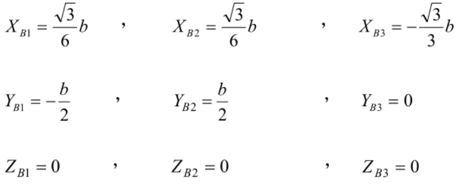
2 b XB 6 3 1 = , XB b 6 3 2 = , XB b 3 3 3 =− 2 1 b YB =− , 2 2 b YB = , YB3 =0 0 1 = B Z , ZB2 =0 , ZB3 =0
The coordinates of Q1, Q , Q of the movable plate with respect to the top frame are: 2 3 a xQ 3 3 1 = , xQ a 6 3 2 =− , xQ a 6 3 3 =− 0 1 = Q y , 2 2 a yQ = , 2 3 a yQ =− 0 1 = Q z , zQ2 =0 , zQ3 =0
The homogeneous transformation from the top to the base frames is described by the transformation matrix:
⎥ ⎥ ⎥ ⎥ ⎦ ⎤ ⎢ ⎢ ⎢ ⎢ ⎣ ⎡ − − + = 1 0 0 0 cos cos cos sin sin cos sin sin sin cos cos cos sin sin sin sin cos sin sin cos cos sin sin cos cos ] [ Z Y X Top Base P P P T β α β α β γ α γ β α γ α γ β α γ α γ β α γ β α γ β ⎥ ⎥ ⎥ ⎢ = v w P ⎥ ⎦ ⎤ ⎢ ⎢ ⎢ ⎣ ⎡ 1 0 0 0 Z z z z Y y y y X x X X P w v u u P w v u (2.1)
The coordinates of the origin of the top frame with respect to the base frame are denoted by [P 、PY、P ]T. Let
X Z α, β , γ represent the rotation
angles defined by rotating the top frame first about the X axis with α degrees, then about the Y axis with β degrees, and finally about the Z axis with γ degrees, respectively. The coordinates of Q , =1, 2, 3, in terms of the base frame can be calculated through
⎥ ⎥ ⎥ ⎥ ⎦ ⎤ ⎢ ⎢ ⎢ ⎢ ⎣ ⎡ = ⎥ ⎥ ⎥ ⎥ ⎦ ⎤ ⎢ ⎢ ⎢ ⎢ ⎣ ⎡ 1 ) , , , , , ]( [ 1 Qi Qi Qi Z Y X Top Base Qi Qi Qi z y x P P P T Z Y X γ β α , i=1~3 (2.2)
Consequently, the coordinates of Q , , and Q with respect to the base frame can be computed
1 Q2 3 ⎥ ⎥ ⎥ ⎥ ⎦ ⎤ ⎢ ⎢ ⎢ ⎢ ⎣ ⎡ = ⎥ ⎥ ⎥ ⎥ ⎦ ⎤ ⎢ ⎢ ⎢ ⎢ ⎣ ⎡ 1 z y x ] [T 1 Z Y X Q1 Q1 Q1 Top Base Q1 Q1 Q1 ⎥ ⎥ ⎥ ⎥ ⎥ ⎦ ⎤ ⎢ ⎢ ⎢ ⎢ ⎢ ⎣ ⎡ ⎥ ⎥ ⎥ ⎥ ⎦ ⎤ ⎢ ⎢ ⎢ ⎢ ⎣ ⎡ = 1 0 0 3 3 1 0 0 0 a P w v u P w v u P w v u Z z z z Y y y y X x x x ⎥ ⎥ ⎢ ⎢ − 3 3 z u P ⎥ ⎥ ⎥ ⎥ ⎥ ⎦ ⎤ ⎢ ⎢ ⎢ ⎢ ⎢ ⎣ ⎡ + + 1 3 3 3 3 Z y Y X X a u a P u a P = (2.3)
⎥ ⎥ ⎥ ⎥ ⎦ ⎤ ⎢ ⎢ ⎢ ⎢ ⎣ ⎡ = ⎥ ⎥ ⎥ ⎥ ⎦ ⎤ ⎢ ⎢ ⎢ ⎢ ⎣ ⎡ 1 z y x ] [T 1 Z Y X Q2 Q2 Q2 Top Base Q2 Q2 Q2 ⎥ ⎥ ⎥ ⎥ ⎥ ⎥ ⎦ ⎤ ⎢ ⎢ ⎢ ⎢ ⎢ ⎢ ⎣ ⎡ − ⎥ ⎥ ⎥ ⎥ ⎦ ⎤ ⎢ ⎢ ⎢ ⎢ ⎣ ⎡ = 1 0 2 6 3 1 0 0 0 a a P w v u P w v u P w v u Z z ⎥ ⎥ ⎢ ⎢ 6 2 z ⎥ ⎥ ⎢ ⎢ − + 1 2 6 z z Z u v P ⎥ ⎥ ⎥ ⎥ ⎦ ⎤ ⎢ ⎢ ⎢ ⎢ ⎣ ⎡ + − + − 1 3 3 2 6 3 z Z y y Y X X X v a u a P a a v a u a P ⎥ ⎥ ⎢ ⎢ − + = P 6 u 2v ⎥ ⎥ ⎢ ⎢ − + = PY 6 uy 2vy ⎥ ⎥ ⎥ ⎥ ⎦ ⎤ ⎢ ⎢ ⎢ ⎢ ⎣ ⎡ + − 3 3 2 6 3 X X X a a a a v a u a P ⎥ ⎥ ⎥ ⎥ ⎦ ⎤ ⎢ ⎢ ⎢ ⎢ ⎣ ⎡ = ⎥ ⎥ ⎥ ⎥ ⎦ ⎤ ⎢ ⎢ ⎢ ⎢ ⎣ ⎡ 1 z y x ] [T 1 Z Y X Q2 Q2 Q2 Top Base Q2 Q2 Q2 ⎥ ⎥ ⎥ ⎥ ⎥ ⎥ ⎦ ⎤ ⎢ ⎢ ⎢ ⎢ ⎢ ⎢ ⎣ ⎡ − ⎥ ⎥ ⎥ ⎥ ⎦ ⎤ ⎢ ⎢ ⎢ ⎢ ⎣ ⎡ = 1 0 2 6 3 1 0 0 0 a a P w v u P w v u P w v u Z z z z Y y y y X x x x (2.4) ⎥ ⎥ ⎥ ⎥ ⎦ ⎤ ⎢ ⎢ ⎢ ⎢ ⎣ ⎡ = ⎥ ⎥ ⎥ ⎥ ⎦ ⎤ ⎢ ⎢ ⎢ ⎢ ⎣ ⎡ 1 z y x ] [T 1 Z Y X Q3 Q3 Q3 Top Base Q3 Q3 Q3
⎥ ⎥ ⎥ ⎥ ⎥ ⎥ ⎦ ⎤ ⎢ ⎢ ⎢ ⎢ ⎢ ⎢ ⎣ ⎡ − ⎥ ⎥ ⎥ ⎥ ⎦ ⎤ ⎢ ⎢ ⎢ ⎢ ⎣ ⎡ = 1 02 6 3 1 0 0 0 a a P w v u P w v u P w v u Z z z z Y y y y X x x x ⎥ ⎥ ⎥ ⎥ ⎥ ⎥ ⎥ ⎢ ⎢ 3 a ⎥ ⎦ ⎢ ⎢ ⎢ ⎢ ⎢ ⎢ ⎣ − − − − − − = 1 2 6 3 2 6 2 6 z z Z y y Y X X X v a u a P v u a P v u a P ⎤ ⎡ 3 a (2.5)
Figure 2.3 illustrates a ball joint has two adjacent equal-length linkages connected to two sliders movable on one of the three guideways mounted on the stationary plate. is the ball joint. and are linear sliders. The length of is b. and are the linkages with a length . Then i Q S2i−1 S2i i 2 B B2i−1 QiF2i−1 QiF2i l i i i i t b t b t22 = 22−1+ 2 −2 2−1 cosϕ , 3i=1~ ] 2 [ cos 1 2 2 2 2 1 2 1 b t b t t i i i i − − − − + = ϕ (2.6) i 1 i 2 1 i 2 2 1 i 2 2 1 i 2 2 t Sˆ 2t Sˆ cos l = − + − − − − ϕ , the distance between B2i and S2i−1 yields
i 2 2 1 i 2 2 i 1 i 2 1 i 2 t cos l t sin Sˆ − = − ϕ − − − ϕ , 3i=1~ (2.7) i i 2 1 i 2 2 i 2 2 1 i 2 2 t (b Sˆ ) 2t (b Sˆ )cos l = − + − − − − ϕ ,
i 2 2 1 i 2 2 i 1 i 2 (b t cos ) l t sin Sˆ = − ϕ − − − ϕ , 3i=1~ (2.8) §2-3 Kinematics of RSSR Mechanisms
The conventional forward kinematics for the six degree-of-freedom manipulator needs complicated mathematic operations. The forward kinematic problem involves systems of highly non-linear equations. Many of these studies was established on the basis of a simplified structure to reduce the nonlinearity of the equations, such that an analytical approach can be performed to complete the solution set.
The proposed forward kinematics used in this chapter needs at first to decomposite the hexglider parallel manipulator into three sets of RSSR structures. After deriving the kinematic relationships existing at the RSSR mechanism mounting on any guideway of the hexglider parallel manipulator, we can intergrate all of the three ones and solve the simultaneous equations to describe the behavior of the hexglider manipulator.
As shown in Figure 2.4, the positions of the ball joints U1 and U2 can be expressed as follows: ⎥ ⎥ ⎥ ⎦ ⎤ ⎢ ⎢ ⎢ ⎣ ⎡ − ⋅ − = r y Rot f Trans U 0 0 ) , ( ) 0 , , 0 ( 1 θ (2.9)
⎥ ⎥ ⎥ ⎦ ⎤ ⎢ ⎢ ⎢ ⎣ ⎡ ⋅ − ⋅ − = q y Rot g Trans z Rot U o 0 0 ) , ( ) 0 , , 0 ( ) 60 , ( 2 δ (2.10)
The distance between U1 and U2 yields
) ( Sin ) ( qrSin ) ( grSin 3 ) ( fqSin 3 ) ( Sin ) ( qrSin 2 fg r q g f b2 2 2 2 2 θ δ θ δ θ δ + − − − − + + + = (2.11)
Eq (2.11) can be expressed as follows
) )Sin( qrSin( ) grSin( 3 ) fqSin( 3 ) )Sin( 2qrSin( fg b r q g f F* 2 2 2 2 2 θ δ θ δ θ δ + − − − − − + + + = (2.12)
Thus, the approximate attitude angles θ 、δ 、φ , as shown in Fig 2.5, can be
computeded by Newton-Raphson method.
§2-4 Newton-Raphson Method
Consider a system of equations . Using the Taylor series
⎪ ⎩ ⎪ ⎨ ⎧ = = = 0 ) , , ( 0 ) , , ( 0 ) , , ( 3 2 1 φ δ θ φ δ θ φ δ θ F F F
expansion with respect to F1(θ,δ,φ),F2(θ,δ,φ),F3(θ,δ,φ) about the current point )
, , ( 0 0 0 0 θ δ φ
X and nelecting terms of order two and higher, we obtain
⎪ ⎪ ⎪ ⎩ ⎪ ⎪ ⎪ ⎨ ⎧ − ∂ + − ∂ + − ∂ ≈ − − ∂ + − ∂ + − ∂ ≈ − − ∂ ∂ + − ∂ ∂ + − ∂ ∂ ≈ − ) ( ) , , ( ) ( ) , , ( ) ( ) , , ( ) , , ( ) ( ) , , ( ) ( ) , , ( ) ( ) , , ( ) , , ( ) ( ) , , ( ) ( ) , , ( ) ( ) , , ( ) , , ( 0 0 0 0 3 0 0 0 0 3 0 0 0 0 3 0 0 0 3 0 0 0 0 2 0 0 0 0 2 0 0 0 0 2 0 0 0 2 0 0 0 0 1 0 0 0 0 1 0 0 0 0 1 0 0 0 1 φ φ φ δ δ δ θ θ θ φ δ θ φ φ φ δ θ δ δ φ δ θ θ θ φ δ θ φ δ θ φ φ φ φ δ θ δ δ δ φ δ θ θ θ θ φ δ θ φ δ θ F F F F F F F F F F F F ∂ ∂ ∂ ∂ ∂ ∂ φ δ θ φ δ θ φ δ θ φ δ θ
(2.13) As described above, a system of equations is given by
⎪ ⎩ ⎪ ⎨ ⎧ = = = 0 ) , , ( 0 ) , , ( 0 ) , , ( 3 2 1 φ δ θ φ δ θ φ δ θ F F F
Applying the Taylor series expansions of F1(θ,δ,φ),F2(θ,δ,φ),F3(θ,δ,φ)about the point Xi(θi,δi,φi)and letting (θ,δ,φ )=(θi+1,δi+1,φi+1), we obtain
⎪ ⎪ ⎪ ⎩ ⎪ ⎪ ⎪ ⎨ ⎧ − ∂ ∂ + − ∂ ∂ + − ∂ ∂ = − − ∂ ∂ + − ∂ ∂ + − ∂ ∂ = − − ∂ ∂ + − ∂ ∂ + − ∂ ∂ = − + + + + + + + + + ) ( ) , , ( ) ( ) , , ( ) ( ) , , ( ) , , ( ) ( ) , , ( ) ( ) , , ( ) ( ) , , ( ) , , ( ) ( ) , , ( ) ( ) , , ( ) ( ) , , ( ) , , ( 1 3 1 3 1 3 3 1 2 1 2 1 2 2 1 1 1 1 1 1 1 i i i i i i i i i i i i i i i i i i i i i i i i i i i i i i i i i i i i i i i i i i i i i i i i i i i i i i F F F F F F F F F F F F φ φ φ φ δ θ δ δ δ φ δ θ θ θ θ φ δ θ φ δ θ φ φ φ φ δ θ δ δ δ φ δ θ θ θ θ φ δ θ φ δ θ φ φ φ φ δ θ δ δ δ φ δ θ θ θ θ φ δ θ φ δ θ (2.14) The system of equations in this study is given by
⎪ ⎩ ⎪ ⎨ ⎧ = = = = = = 0 ) , ( ) , , ( 0 ) , ( ) , , ( 0 ) , ( ) , , ( 1 3 1 2 1 1 i i i i i i i i i i i i i i i F F F F F F θ φ φ δ θ φ δ φ δ θ δ θ φ δ θ (2.15)
To differential F1(θ,δ,φ),F2(θ,δ,φ),F3(θ,δ,φ) with respect to φ, θ, δ yields
0 ) , ( ) , , ( 1 1 = ∂ ∂ = ∂ ∂ φ δ θ φ φ δ θi i i F i i F 0 ) , ( ) , , ( 2 2 = ∂ ∂ = ∂ ∂ θ φ δ θ φ δ θi i i F i i F 0 ) , ( ) , , ( 3 3 = ∂ ∂ = ∂ ∂ δ θ φ δ φ δ θi i i F i i F
⎪ ⎪ ⎪ ⎩ ⎪ ⎪ ⎪ ⎨ ⎧ − ∂ ∂ + − ∂ ∂ = − = − − ∂ ∂ + − ∂ ∂ = − = − − ∂ ∂ + − ∂ ∂ = − = − + + + + + + ) ( ) , ( ) ( ) , ( ) , ( ) , , ( ) ( ) , ( ) ( ) , ( ) , ( ) , , ( ) ( ) , ( ) ( ) , ( ) , ( ) , , ( 1 3 1 3 3 3 1 2 1 2 2 2 1 1 1 1 1 1 i i i i i i i i i i i i i i i i i i i i i i i i i i i i i i i i i i i i i i i F F F F F F F F F F F F θ θ φ φ θ φ φ θ φ θ φ θ φ δ θ φ φ φ φ δ δ δ δ φ δ φ δ φ δ θ δ δ δ δ θ θ θ θ δ θ δ θ φ δ θ (2.16)
The determinant D is presently equalent to the Jocobian matrix of F1(θ,δ,φ),
) , , ( 2 θ δ φ F ,F3(θ,δ,φ) and denoted by (2.17) To apply Cramer’s rule, we can obtain the solutions of the above linear system of equations ∆θi, ∆δi, ∆φi as follows
D F 0 F F F F 0 F F i i 3 i i 3 i i 2 i i 2 i i 2 i i 1 i i 1 i 1 i i φ θ φ θ φ φ φ δ δ φ δ φ δ δ δ θ δ θ θ θ θ ∆ ∂ ∂ − ∂ ∂ ∂ ∂ − ∂ ∂ − = − = + ) , ( ) , ( ) , ( ) , ( ) , ( ) , ( ) , ( θ θ φ φ φ δ δ δ θ φ θ φ δ φ δ θ δ θ ∂ ∂ ∂ ∂ ∂ ∂ + ∂ ∂ ∂ ∂ ∂ ∂ = i i i i i i φ θ φ θ θ φ φ φ δ δ φ δδ δ θ θ δ θ φ δ θ φ δ θ φ δ θ φ φ δ θ δ φ δ θ θ φ δ θ φ φ δ θ δ φ δ θ θ φ δ θ ∂ ∂ ∂ ∂ ∂ ∂ ∂ ∂ ∂ ∂ ∂ ∂ = ∂ ∂ ∂ ∂ ∂ ∂ ∂ ∂ ∂ ∂ ∂ ∂ ∂ ∂ ∂ = ) , ( ) , ( ) , ( ) , ( ) , ( ) , ( ) , ( 0 ) , ( ) , ( ) , ( 0 0 ) , ( ) , ( ) , , ( ) , , ( ) , , ( ) , , ( ) , , ( ) , , ( ) , , ( ) , , ( ) , , ( 3 2 1 3 2 1 3 3 2 2 1 1 3 3 3 2 2 2 1 1 1 i i i i i i i i i i i i i i i i i i i i i i i i i i i i i i i i i i i i i i i i i i i i i F F F F F F F F F F F F F F F F F F F F F φ δ θ ∂ ∂ ∂ D
θ θ φ φ φ δ δ δ θ φ θ φ δ φ δ θ δ θ φ θ φ δ δ θ φ δ φ φ δ δ δ θ θ φ φ θ φ δ φ δ δ θ ∂ ∂ ∂ ∂ ∂ ∂ + ∂ ∂ ∂ ∂ ∂ ∂ ∂ ∂ ∂ ∂ + ∂ ∂ ∂ ∂ − ∂ ∂ ∂ ∂ − = ) , ( ) , ( ) , ( ) , ( ) , ( ) , ( ) , ( ) , ( ) , ( ) , ( ) , ( ) , ( ) , ( ) , ( ) , ( i i 3 i i 2 i i 1 i i 3 i i 2 i i 1 i i 3 i i 1 i i 2 i i 2 i i 1 i i 3 i i 3 i i 2 i i 1 F F F F F F F F F F F F F F F (2.18) θ θ φ φ φ δ δ δ θ φ θ φ δ φ δ θ δ θ θ δ θ φ φ δ θ φ θ θ φ φ φ δ δ θ θ δ θ φ θ φ φ δ φ θ φ θ φ θ θ φ φ φ δ φ δ δ θ θ δ θ δ δ δ ∂ ∂ ∂ ∂ ∂ ∂ + ∂ ∂ ∂ ∂ ∂ ∂ ∂ ∂ ∂ ∂ + ∂ ∂ ∂ ∂ − ∂ ∂ ∂ ∂ − = ∂ ∂ − ∂ ∂ ∂ ∂ − − ∂ ∂ = − = ∆ + ) , ( ) , ( ) , ( ) , ( ) , ( ) , ( ) , ( ) , ( ) , ( ) , ( ) , ( ) , ( ) , ( ) , ( ) , ( ) , ( ) , ( ) , ( ) , ( ) , ( 0 0 ) , ( ) , ( 3 2 1 3 2 1 1 2 3 3 2 1 1 3 2 3 3 3 2 2 1 1 1 i i i i i i i i i i i i i i i i i i i i i i i i i i i i i i i i i i i i i i i i i i i i i i i F F F F F F F F F F F F F F F D F F F F F F F (2.19) θ θ φ φ φ δ δ δ θ φ θ φ δ φ δ θ δ θ δ φ δ θ θ φ δ θ δ δ θ θ θ φ φ δ δ φ δ θ δ θ θ φ θ φ θ θ φ φ δ δ φ δ δ θ δ δ θ θ δ θ φ φ φ ∂ ∂ ∂ ∂ ∂ ∂ + ∂ ∂ ∂ ∂ ∂ ∂ ∂ ∂ ∂ ∂ + ∂ ∂ ∂ ∂ − ∂ ∂ ∂ ∂ − = − ∂ ∂ − ∂ ∂ − ∂ ∂ ∂ ∂ = − = ∆ + ) , ( ) , ( ) , ( ) , ( ) , ( ) , ( ) , ( ) , ( ) , ( ) , ( ) , ( ) , ( ) , ( ) , ( ) , ( ) , ( 0 ) , ( ) , ( ) , ( 0 ) , ( ) , ( ) , ( 3 2 1 3 2 1 2 3 1 1 3 2 2 1 3 3 3 2 2 1 1 1 1 i i i i i i i i i i i i i i i i i i i i i i i i i i i i i i i i i i i i i i i i i i i i i i i F F F F F F F F F F F F F F F D F F F F F F F (2.20) The recursive formulus yields
⎪
⎩
⎪
⎨
⎧
∆
+
=
∆
+
=
∆
+
=
+ + + i i i i i i i i iφ
φ
φ
δ
δ
δ
θ
θ
θ
1 1 1 1 (2.21)If initial points θ0,δ0,φ0 are given, θ ,
δ
,φ
can be computed by recursive operations.§2-5 Forward Kinematics
Applying Eq (2.11) to the forward kinematic analysis of the hexglider manipulator, a system of equation with respect to the attitude angles θ, δ , and φ can be obtained ⎪ ⎪ ⎩ ⎪⎪ ⎨ ⎧ = = = 0 r r g f F 0 r r g f F 0 r r g f F 1 3 3 3 3 2 2 2 2 1 1 1 ) , , , , , ( ) , , , , , ( ) , , , , , ( * * *
δ
φ
φ
δ
δ
θ
(2.22)As shown in Figure 2.5, the coordinates of ball joint U1, U2, U3 on the upper plate can be computeded with the solved attitude angles θ , δ , and φ
⎥ ⎥ ⎥ ⎦ ⎤ ⎢ ⎢ ⎢ ⎣ ⎡ − ⋅ − = 1 1 0 0 ) , ( ) 0 , 3 , ( 1 r y Rot f BR BR Trans U θ (2.23) ⎥ ⎥ ⎥ ⎦ ⎤ ⎢ ⎢ ⎢ ⎣ ⎡ − ⋅ − ⋅ = 2 2 0 0 ) , ( ) 0 , 3 , ( ) 120 , ( 2 r y Rot f BR BR Trans z Rot U o δ (2.24)
⎥ ⎥ ⎥ ⎦ ⎤ ⎢ ⎢ ⎢ ⎣ ⎡ − ⋅ − ⋅ = 3 3 0 0 ) , ( ) 0 , 3 , ( ) 240 , ( 3 r y Rot f BR BR Trans z Rot U o φ (2.25)
Substituting the coordinates of ball joints U1, U2, U3 into Eq.(2.26), the coordinates of the center of the end-effector px, py, and pz can be obtained as follows ⎥ ⎥ ⎥ ⎦ ⎤ ⎢ ⎢ ⎢ ⎣ ⎡ − + + = ⎥ ⎥ ⎥ ⎦ ⎤ ⎢ ⎢ ⎢ ⎣ ⎡ IH U U U p p p z y x 0 0 3 / ) 3 2 1 ( (2.26)
The Euler rotation matrix Eq.(2.27) denotes a set of unit base vecters of the coordinate system describing the pose of the end-effector
⎥
⎥
⎥
⎦
⎤
⎢
⎢
⎢
⎣
⎡
=
⎥
⎥
⎥
⎦
⎤
⎢
⎢
⎢
⎣
⎡
−
−
+
+
−
=
⋅
⋅
=
z z z y y y x x xw
v
u
w
v
u
w
v
u
cos
cos
sin
cos
sin
sin
cos
cos
sin
sin
cos
cos
sin
sin
sin
cos
sin
sin
sin
cos
sin
cos
cos
sin
sin
sin
cos
cos
cos
)
,
x
(
Rot
)
,
y
(
Rot
)
,
z
(
Rot
)
,
,
(
RPY
α
β
α
β
β
α
γ
α
β
γ
α
γ
α
β
γ
β
γ
α
γ
α
β
γ
α
γ
α
β
γ
β
γ
α
β
γ
α
β
γ
(2.27) As a result, the positions of ball joints U1, U2, and U3 with respect to the coordinates of the center of the end-effector px, py, and pz, the radius of the tangent circle of the equilateral-triangle UR, and the unit pose vectors of the end-effector , , can be derived as Eq.(2.28), Eq.(2.29), and1
Q Q2Q3 u u u
Eq.(2.30). ⎥ ⎥ ⎥ ⎦ ⎤ ⎢ ⎢ ⎢ ⎣ ⎡ ⋅ + ⋅ + ⋅ + = z z y y x x u UR p u UR p u UR p 1 U (2.28) ⎥ ⎥ ⎥ ⎥ ⎥ ⎥ ⎥ ⎦ ⎤ ⎢ ⎢ ⎢ ⎢ ⎢ ⎢ ⎢ ⎣ ⎡ ⋅ + ⋅ − ⋅ + ⋅ − ⋅ + ⋅ − = z z z y y y x x x v UR u UR p v UR u UR p v UR u UR p U 2 3 2 1 2 3 2 1 2 3 2 1 2 (2.29) ⎥ ⎥ ⎥ ⎥ ⎥ ⎥ ⎥ ⎦ ⎤ ⎢ ⎢ ⎢ ⎢ ⎢ ⎢ ⎢ ⎣ ⎡ ⋅ − ⋅ − ⋅ − ⋅ − ⋅ − ⋅ − = z z z y y y x x x v UR u UR p v UR u UR p v UR u UR p U 2 3 2 1 2 3 2 1 2 3 2 1 3 (2.30)
Rewrite Eq.(2.28), Eq.(2.29), and Eq.(2.30), γ , β , and α can be
computed from Eq.(2.31), Eq.(2.32), and Eq.(2.33). ) 1 1 ( 1 x x y y p U p U Tan − − = − γ (2.31) ) 1 ( 1 UR p IH U Sin z − − z = − β (2.32) ) 3 3 2 ( 1 β α Cos UR U U Sin z z ⋅ − = − (2.33)
Chapter 3
Modeling of Motion Errors
§3.1 Introduction
The SP-120 is a six degree of freedom parallel manipulator which is presently the one used for modeling the false circular cotour of motion errors resulting from the individual error sources of the manipulater. With the results of simplified forward kinematics, the position deviations generated by geometric error sources, especially assembly errors, are derived mathmatically in this chapter. Simutaneously, the parameter errors relating to the geometric error sources are described as well.
§3.2 Error Descriptions
All of the errors are coupled in any parallel manipulator. Therefore, the total possible errors can be summed and expressed in terms of the Taylor expansion as follows: Total error ) ( ... ) ( ) ( ) ..., , , ( , x E c x E c x E c c c c x E m m 2 2 1 1 m 2 1 + + + = = (3.1)
Geometric resources of motional deviations, including translate and angular ones, resulting from the manufacturing or assembly of guideways and linkages
are classified and modeled with the analytical results of the kinematics in the thesis.
As shown in Fig 3.1, the geometric resources of motional deviations under investigation can be classified and described as follows.
(1) Linkage length error
The length errors of the six linkages due to the the manufacturing tolerances may affect the pose accuracy of the manipulator.
(2) Slider positioning error
The positioning errors of the six sliders S1 to S6 are usually generated from the controller, and they might exist at the initialized command data.
(3) Assembly errors for the guideways
Three guideways are assembled on the stationary plate. Three ball joints are mounted on the mobile plate as well. The improper positions of fixing guideways or ball joints may lead to assembly errors. The assembly errors can be categorized into the following items:
1. Guideway translation error ﹔In Figure 3.2 (a), the guideway is
translated a positional error along the X , Y , or Z axis.
2. Guideway rotation error (I) ﹔In Figure 3.2 (b), the guideway is
rotated an angular error by the center of the guide way on XY or YZ plane.
3. Guideway rotation error (II) ﹔In Figure 3.2 (c), the guideway is rotated an angular error about the center of the tri-angle, consist of three guideways and fixed on the base plate, on XY plane. The angular and positional deviations of the end-effector in the machine coordinate system are defined. There are thirty three deviations in a hexglider manipulator. In the following, We begin to model the above deviations with the analytical results of the kinematics.
§3.3 Error Modeling
(1) Translation errors of the guide way
a) Translation error along X-axis
[Type I]
In Figure 3.3, a translation error λXI along the X-axis of the
ight guideway is added. The position of the ball joint U2 is taken from Eq.(2.10), and the true position of the ball joint U1 becomes
1 U ) 0 , 0 , ( Trans ' 1 U = λXI ⋅ (3.2) After simplifing the equation, the distance between U1’ and U2 yields
) rSin 2 qSin g 3 ( Cos qrCos 2 Sin qrSin fqSin 3 grSin 3 fg r q g f b XI 2 2 2 2 2 θ δ λ δ θ δ θ δ θ − − + − + − − − + + + = (3.3) Eq (3.3) can be expressed as
) 2rSin qSin δ g 3 ( 2qrCosCos δ Sin qrSin fqSin δ 3 grSin θ 3 fg b r q g f F XI 2 2 2 2 2 1 θ λ δ θ − − + − + − − − − + + + = (3.4) [Type II]
Figure 3.4 shows a translation error λXII along the X-axis of the left
guideway is added .We can get the position of the ball joint U1 from Eq.(2.9) and derive the true position of the ball joint U2
2 U ) 0 , 2 3 , 2 ( Trans ' 2 U = −λXII λXII ⋅ (3.5)
The distance between U1 and U2’ yields
) qSin 2 rSin f 3 ( Cos qrCos 2 Sin qrSin fqSin 3 grSin 3 fg r q g f b XII 2 2 2 2 2 δ θ λ δ θ δ θ δ θ − − + − + − − − + + + = (3.6) Eq (3.5) can be expressed as ) 2qSin rSin θ f 3 ( δ 2qrCos θqrC Sin qrSin fqSin δ 3 grSin θ 3 fg b r q g f F XII 2 2 2 2 2 2 δ λ δ θ − − + − + − − − − + + + = (3.7)
b) Translation error along Y-axis
[Type I]
In Figure 3.5, a translation error λYI along the Y-axis of the
right guideway is added. The position of the ball joint U2 remains the same and is taken from Eq.(2.10). The true position of the ball joint U1 becomes
1 U ) 0 , , 0 ( Trans ' 1 U = λYI ⋅ (3.8)
Simplify the distance b between U1’ and U2 and obtain ) qSin 3 f 2 g ( Cos qrCos 2 Sin qrSin fqSin 3 grSin 3 fg r q g f b YI 2 2 2 2 2 δ λ δ θ δ θ δ θ − − + − + − − − + + + = (3.9) Eq (3.9) can be expressed as ) qSin 3 2f (g Cosδ 2qrCos Sin qrSin fqSin δ 3 grSin θ 3 fg b r q g f F YI 2 2 2 2 2 3 δ λ θ δ θ − − + − + − − − − + + + = (3.10) [Type II]
Figure 3.6 shows a translation error λ along the Y-axis of the left YII
guideway is added .We can get the position of the ball joint U1 form Eq.(2.9) and derive the true position of the ball joint U2
⎥ ⎥ ⎥ ⎦ ⎤ ⎢ ⎢ ⎢ ⎣ ⎡ ⋅ + − ⋅ − = q 0 0 ) , y ( Rot ) 0 , g , 0 ( Trans ) 60 , z ( Rot ' 2 U o λYII δ (3.11)
Simplify the distance b between U1 and U2’ and obtain
) rSin 3 g 2 f ( Cos qrCos 2 Sin qrSin fqSin 3 grSin 3 fg r q g f b YII 2 2 2 2 2 θ λ δ θ δ θ δ θ − − + − + − − − + + + = (3.12) Eq (3.12) can be expressed as ) rSin 3 2g (f Cos 2qrCos Sin qrSin fqSinδ 3 grSinθ 3 fg b r q g f F YII 2 2 2 2 2 4 θ λ δ θ δ θ − − + − + − − − − + + + = (3.13)
[Type I]
In Figure 3.7, a translation error λ along the Z-axis of the ZI
right guideway is added. The position of the ball joint U2 remains the same and is taken from Eq.(2.10). The true position of the ball joint U1 becomes
1 U ) , 0 , 0 ( Trans ' 1 U = λZI ⋅ (3.14)
Simplify the distance b between U1’ and U2 and obtain
) qCos rCos ( 2 Cos qrCos 2 Sin qrSin fqSin 3 grSin 3 fg r q g f b ZI 2 2 2 2 2 δ θ λ δ θ δ θ δ θ − + − + − − − + + + = (3.15) Eq (3.15) can be expressed as ) qCos (rCos 2 Cos 2qrCos Sin qrSin fqSinδ 3 grSinθ 3 fg b r q g f F ZI 2 2 2 2 2 5 δ θ λ δ θ δ θ − + − + − − − − + + + = ( 3.16) [Type II]
Figure 3.8 shows a translation error λ along the Z-axis of the left ZII
guideway is added .We can get the position of the ball joint U1 form eq.(2.9) and derive the true position of the ball joint U2
2 U ) , 0 , 0 ( Trans ' 2 U = λZII ⋅ (3.17)
The distance between U1 and U2’ yields
) qCos rCos ( 2 Cos qrCos 2 Sin qrSin fqSin 3 grSin 3 fg r q g f b ZII 2 2 2 2 2 δ θ λ δ θ δ θ δ θ − − − + − − − + + + = (3.18) Eq (3.18) can be expressed as
) qCos rCos ( 2 Cos qrCos 2 Sin qrSin fqSin 3 grSin 3 fg b r q g f F ZII 2 2 2 2 2 6 δ θ λ δ θ δ θ δ θ − − − + − − − − + + + = (3.19)
(2) Rotation errors of the Guide way
a) Rotatation error on XY plane
[Type I]
In Figure 3.9, a rotatation error εXYI on the XY-plane is added to the
right guideway. The position of the ball joint U2 remains the same and is taken from Eq.(2.10). The true position of the ball joint U1 becomes
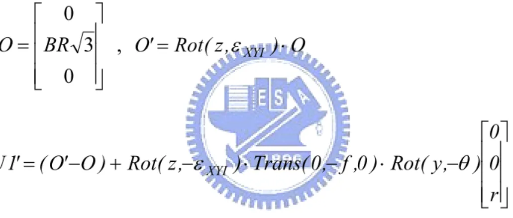
⎥ ⎥ ⎥ ⎦ ⎤ ⎢ ⎢ ⎢ ⎣ ⎡ = 0 3 0 BR O , O'= Rot(z,εXYI )⋅O ⎥ ⎥ ⎥ ⎦ ⎤ ⎢ ⎢ ⎢ ⎣ ⎡ − ⋅ − ⋅ − + − = r 0 0 ) , y ( Rot ) 0 , f , 0 ( Trans ) , z ( Rot ) O ' O ( ' 1 U εXYI θ (3.20)
Simplify the distance b between U1’ and U2 and obtain
] ) ) [ θ δ θ δ ε δ θ δ θ δ θ Sin qrSin 3 qSin f BR 3 ( rSin g BR 3 2 ( f BR 3 fg 3 Cos qrCos 2 Sin qrSin fqSin 3 grSin 3 fg r q g f b XYI 2 2 2 2 2 + + ⋅ + + ⋅ + ⋅ ⋅ − − + − + − − − + + + = (3.21) Eq (3.21) can be expressed as ] ) ) [ θ δ θ δ ε δ θ δ θ δ θ Sin qrSin 3 qSin f BR 3 ( rSin g BR 3 2 ( f BR 3 fg 3 Cos qrCos 2 Sin qrSin fqSin 3 grSin 3 fg b r q g f F XYI 2 2 2 2 2 7 + + ⋅ + + ⋅ + ⋅ ⋅ − − + − + − − − − + + + = (3.22) [Type II]
the guideway B2B3. We can get the position of the ball joint U1 form Eq.(2.9) and derive the true position of the ball joint U2
⎥ ⎥ ⎥ ⎥ ⎥ ⎥ ⎦ ⎤ ⎢ ⎢ ⎢ ⎢ ⎢ ⎢ ⎣ ⎡ = 0 2 3 2 3 BR BR O , O' = Rot(z,−εXYII )⋅O ⎥ ⎥ ⎥ ⎦ ⎤ ⎢ ⎢ ⎢ ⎣ ⎡ ⋅ − ⋅ − − + − = q 0 0 ) , y ( Rot ) 0 , g , 0 ( Trans ) 60 , z ( 1 Rot ) O ' O ( ' 2 U o εXYII δ (3.23) Simplify the distance b between U1 and U2’ and obtain
] ) ) [ θ δ θ δ ε δ θ δ θ δ θ Sin qrSin 3 qSin f BR 3 2 ( rSin g BR 3 ( f BR 3 fg 3 Cos qrCos 2 Sin qrSin fqSin 3 grSin 3 fg r q g f b XYII 2 2 2 2 2 − − ⋅ + − ⋅ + ⋅ ⋅ + − + − + − − − + + + = (3.24) Eq (3.24) can be expressed as ] ) ) [ θ δ θ δ ε δ θ δ θ δ θ Sin qrSin 3 qSin f BR 3 2 ( rSin g BR 3 ( f BR 3 fg 3 Cos qrCos 2 Sin qrSin fqSin 3 grSin 3 fg b r q g f F XYII 2 2 2 2 2 8 − − ⋅ + − ⋅ + ⋅ ⋅ + − + − + − − − − + + + = (3.25)
b) Rotatation error on YZ plane
[Type I]
In Figure 3.11, a rotatation error ε on the YZ-plane is added to the YZI
right guideway. The position of the ball joint U2 remains the same and is taken from Eq.(2.10). The true position of the ball joint U1 becomes
⎥ ⎥ ⎥ ⎦ ⎤ ⎢ ⎢ ⎢ ⎣ ⎡ = 0 3 0 BR O , O'= Rot(x,εYZI )⋅O ⎥ ⎥ ⎥ ⎦ ⎤ ⎢ ⎢ ⎢ ⎣ ⎡ − ⋅ − ⋅ − + − = r 0 0 ) , y ( Rot ) 0 , f , 0 ( Trans ) , x ( Rot ) O ' O ( ' 1 U εYZI θ (3.26)
Simplify the distance b between U1’ and U2 and obtain
] [ θ δ δ θ δ ε δ θ δ θ δ θ Sin qrSin 3 Cos ) q r ( BR 3 2 fqSin grSin fg 3 Cos qrCos 2 Sin qrSin fqSin 3 grSin 3 fg r q g f b YZI 2 2 2 2 2 + − ⋅ ⋅ + + + − + − + − − − + + + = (3.27) Eq (3.27) can be expressed as ] [ θ δ δ θ δ ε δ θ δ θ δ θ Sin qrSin 3 Cos ) q r ( BR 3 2 fqSin grSin fg 3 Cos qrCos 2 Sin qrSin fqSin 3 grSin 3 fg b r q g f F YZI 2 2 2 2 2 9 + − ⋅ ⋅ + + + − + − + − − − − + + + = (3.28) [Type II]
Figure 3.12 shows a rotatation error εYZII on the YZ-plane is added to
the left guideway. We can get the position of the ball joint U1 form Eq.(2.9) and derive the true position of the ball joint U2
⎥ ⎥ ⎥ ⎦ ⎤ ⎢ ⎢ ⎢ ⎣ ⎡ = 0 3 0 BR O , O' = Rot(x,−εYZII )⋅O ⎥ ⎥ ⎥ ⎦ ⎤ ⎢ ⎢ ⎢ ⎣ ⎡ ⋅ − ⋅ − ⋅ − + − = q 0 0 ) , y ( Rot ) 0 , g , 0 ( Trans ) , x ( Rot ) 60 , z ( Rot ) O ' O ( ' 2 U o εYZII δ (3.29)
Simplify the distance b between U1 and U2’ and obtain ] [ θ δ θ δ ε δ θ δ θ δ θ Sin qrSin 3 qCos ) BR 3 2 f ( rCos ) BR 3 g ( 2 Cos qrCos 2 Sin qrSin fqSin 3 grSin 3 fg r q g f b YZII 2 2 2 2 2 + ⋅ + + ⋅ + − + − + − − − + + + = (3.30) Eq (3.30) can be expressed as ] [ θ δ θ δ ε δ θ δ θ δ θ Sin qrSin 3 qCos ) BR 3 2 f ( rCos ) BR 3 g ( 2 Cos qrCos 2 Sin qrSin fqSin 3 grSin 3 fg b r q g f F YZII 2 2 2 2 2 10 + ⋅ + + ⋅ + − + − + − − − − + + + = (3.31) The deviations due to rotating the guide way on the XZ plane will not be derived because the joint of the RSSR mechanism is free.
(c) Rotatation error about the center of the base on XY plane [Type I]
Figure 3.13 shows a rotatation error ε about the center of the base OI
on the XY-plane is added to the right guideway. We can get the position of the ball joint U2 form Eq.(2.9) and derive the true position of the ball joint U1 ⎥ ⎥ ⎥ ⎦ ⎤ ⎢ ⎢ ⎢ ⎣ ⎡ = 0 3 BR BR O O ) , z ( Rot ' O = εOI ⋅ ⎥ ⎥ ⎥ ⎦ ⎤ ⎢ ⎢ ⎢ ⎣ ⎡ − ⋅ − ⋅ + − = r 0 0 ) , y ( Rot ) 0 , f , 0 ( Trans ) , z ( Rot ) ' O O ( 1 U εOI θ (3.32)