sors. Later, some cost-optimal parallel solvers were pre-sented, where cost is defined to be the product of time and the number of processors used [19]. Using a newly proposed computational model called the mesh-of-unshuf-fle network, Chung and Lin [7] presented an O(log m log n)-time parallel algorithm using O(mn/(log m log n)) processors. On a hypercube network, a similar result was presented by Lin and Chung [20]. Using the pipelining strategy [11], an O(log n9)-time parallel algorithm was presented on the same network with O(mn/log n9) proces-sors [13], where n9 5 max(m, n). Cheng et al. [6] presented the first constant-time parallel algorithm on a mesh-con-nected computer with O(mn) processors based on the Chebyshev iterative method; they also gave the corre-sponding relative error analysis. Note that their algorithm [6] is time- and cost-optimal.
Based on the matrix perturbation method, this paper first presents a novel approximate O(n/p)-time parallel B-spline curve fitting algorithm for finding the corresponding
n control points that interpolate those n data points on a
linear array processor with p processors, where p # n. Given m 3 n data points, we then present an O(mn/ ( p1p2))-time parallel algorithm for B-spline surface fitting on a p13 p2mesh-connected computer, where p1# m and
p2# n. The relative error analyses of our two stable and cost-optimal parallel solvers are also given. When setting
p15 m and p25 n, a time- and cost-optimal parallel solver can be derived; our result is a direct method vs. the result of Cheng et al. [6].
2. PARALLEL B-SPLINE CURVE INTERPOLATOR Suppose we are given a set of 3-dimensional data points,
Bi 5 (b (1) i , b (2) i , b (3) i ) for 1# i # n. According to [2, 15],
for uniform B-spline curve, each data point can be ex-pressed by a weighted average of three control points:
Bi 5 Ah(Ci21 1 4Ci 1 Ci11), 1 # i # n, where Ci 5
(c(1)i , c(2)i , c(3)i ). They form a system of n equations in n1 2 unknowns for all given points. In order to completely solve the system, we need the following two additional equations to specify how the boundary control points are interpolated: C05 C1; Cn115 Cn. For simplicity, we only
consider b 5 (b1, b2, ..., bn)T 5 (b(1)1 , b (1) 2 , ..., b (1) n )T and c 5 (c1, c2, ..., cn)T 5 (c(1)1 , c (1) 2 , ..., c (1) n )T throughout this ARTICLE NO.0082
Parallel B-Spline Surface Fitting on Mesh-Connected Computers
KUO-LIANGCHUNG*,1AND WEN-MING YAN†,2
*Department of Information Management, National Taiwan Institute of Technology, No. 43, Section 4, Keelung Road,
Taipei, Taiwan 10672, Republic of China; and †Department of Computer Science and Information Engineering, National Taiwan University, Taipei, Taiwan 10764, Republic of China
0743-7315/96 $18.00 Copyright1996 by Academic Press, Inc. All rights of reproduction in any form reserved.
205
The solution of uniform bicubic B-spline curve/surface fitting problem is considered. Based on the matrix perturbation method, this paper first presents a novel approximate O(n/p)-time parallel B-spline curve fitting algorithm for finding the corresponding n control points that interpolate those n data points on a linear array processor with p processors, where p # n. Given m 3 n data points, we then present an O(mn/
( p1p2))-time parallel algorithm for solving the uniform bicubic
B-spline surface fitting problem on a p13 p2mesh-connected
computer, where p1# m and p2# n. The relative error analyses
of our two stable and cost-optimal parallel solvers are also given. When setting p15 m and p25 n, a constant-time parallel
solver for B-spline surface fitting can be derived; this time- and cost-optimal result is a direct method, in contrast to the parallel iterative method of Cheng et al. (Parallel B-spline surface inter-polation on a mesh-connected processor array, J. Parallel Dis-trib. Comput. 24, 2 (1995), 224–229). 1996 Academic Press, Inc.
1. INTRODUCTION
Surface fitting is very important in the fields of CAD, CAM, robotic path planning, graphics, pattern recognition, and image processing. Due to the local change property, B-spline surface interpolation is a good fitting tool to con-struct a smooth surface that fits those given points in the space [15, 2]. From the viewpoint of filters, finding the control points can be solved by using an inverse filtering operation [17].
Suppose we are given a set of m3 n data points to be interpolated. Based on the Gauss–Seidel iteration method, Ajjanagadde and Patnaik [1] presented the first parallel algorithm to perform uniform bicubic B-spline surface fit-ting in O(n1 p) time using O(pn) processors, where p is the number of iterations specified by the user. Then Cheng and Goshtasby [4] presented another parallel iterative solver based on the SLOR method to find the control points in O(m log n) time using O(n) processors. Based on the cyclic reduction method [18], Cheng and Goshtasby [5] presented the first logarithmic-time parallel algorithm, which takes O(log m1 log n) time using O(mn)
proces-1
E-mail: [email protected].
2
which implies that a2 b 5 4 and 2ab 5 1; this then implies that b5 21/a and a 5 2 6 Ï3. Since we wish the matrices
L9 and U9 to be diagonally dominant, we will select the
sign so that the absolute value of a is greater than 1. There-fore, let a5 2 1 Ï3 and b 5 21/a 5 Ï3 2 2.
The computation of a and b provides the Toeplitz factor-ization of matrix A9q(phase 1 in our algorithm), which can
be computed in parallel by each processor in O(1) time on the array processor.
2.2. Phase 2: Substitution Procedure
Initially, we partition b into p parts and b 5 (b0T, b1T, ..., bp21T)T, where bi5 (6b
iq11, 6biq12, ..., 6biq1q)T
for 0 # i # p 2 1. The ith processor first solves A9qzi5
bi, 0# i # p 2 1, where zi5 (z
iq11, ziq12, ..., ziq1q)T, that
is, the ith processor solves L9qU9qzi5 bi. It can be verified
that each processor in the linear array processor needs about 5q time to perform the forward and backward substi-tution procedure for solving L9qU9qzi5 bi (second phase
in our algorithm) sequentially [16]. Consequently, it follows that
Anz2 b 5 gpen1 hpe11
O
p21 i51 (gieiq1 hieiq11), (4) where gi5 ziq11, hi5 ziq1 (2 2 Ï3)ziq11, 1# i # p 2 1, (5) gp5 zn, hp5 (3 2 Ï3)z1. (6)By (4), the solution of c in (1) will be determined approx-imately, say, z2 p, in Section 2.3 later, where Ap P gpen1 hpe11
o
p21
i51( gieiq1 hieiq11). To estimate the bound of the relative error, we need the following two auxiliary results. Herei ● i denotes the infinity norm of a vector.
LEMMA1 [13]. If Ax5 b, where A 5 [aij]n3nis a diago-nally dominant matrix, then ixi # (1/min1#i#n (uaiiu 2
o
nj51, j?iuaiju)) ibi.
For A9 in (2), because min1#i#n(uaiiu 2
o
nj51, j?iuaiju) 5 2,
we have the immediate result.
COROLLARY2 [13]. If A9x9 5 b9, then ix9i # Asib9i.
From A9qzi5 bifor 0 # i # p 2 1 and by Corollary 2,
izii # Asibii # Asibi. (7)
2.3. Phase 3: Update Procedure
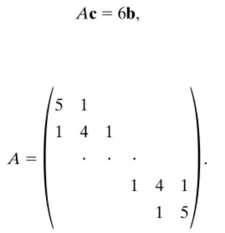
From (4), the solution of c in (1) will be determined approximately in this section and only local communica-section. Thus, the above system of linear equations can be
equivalently transformed into
Ac5 6b, (1) where A5
1
5 1 1 4 1 ? ? ? 1 4 1 1 52
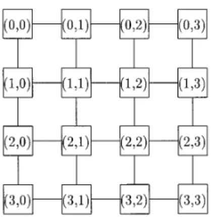
.Our parallel solver consists of three phases called the Toeplitz factorization, the substitution procedure, and the update procedure, respectively. Suppose we have a linear array processor with p processors. Figure 1 shows a linear array processor with four processors, where the processor identity inside the square box denotes the address of the processor. For convenience, suppose n is a multiple of the number of processors used, i.e., n 5 pq. Throughout the remainder of this section, matrices are represented by up-percase letters, vectors by bold lowercase letters, and sca-lars by plain lowercase letters. The superscript T corres-ponds to the transpose operation. We now show how each phase can be accomplished on the linear array network in a highly parallel way.
2.1. Phase 1: Toeplitz Factorization
Let A9q5
1
a 1 1 4 1 ? ? ? 1 4 1 1 42
q3q 5 L9qU9q, (2) L9q51
1 2b 1 ? ? 2b 1 2b 12
q3q , and U9q51
a 1 a 1 ? ? a 1 a2
q3q , (3)tions between adjacent processors on the linear array pro-cessor will be needed. Then, the bound of the relative error will be analyzed.
From a2 b 5 4 and 2ab 5 1, we have 1 1 4b 1 b25 0. Let pk 5 (0, ..., 0, 1, b, ..., b
t, 0, ..., 0)
T and qk 5k n2k
(0, ..., 0, bt, ..., b, 1, 0, ..., 0)T for q # k # n 2 q 1 1.
k n2k
Here we assume that q . t. In addition, we let p1 5 (1, b, ..., bt21, bt, 0, ..., 0)Tand q n5 (0, ..., 0, bt, bt21, ..., b, 1)T. Accordingly, we have Apk5 ek211 (2 1 Ï3)ek1 bt(2bek1t1 ek1t11), (8) Aqk5 bt(ek2t212 bek2t)1 (2 1 Ï3)ek1 ek11, (9) Ap15 (3 1 Ï3)e11 bt(2bet111 et12), (10) Aqn5 (3 1 Ï3)en1 bt(en2t212 ben2t). (11)
By (8), (9), (10), and (11), for 1 # i # p 2 1, we have
A(uipiq111 viqiq)5 (ui1 (2 1 Ï3)vi)eiq
1 ((2 1 Ï3)ui1 vi)eiq11 1 uibt(2beiq1t111 eiq1s12)
1 vibt(eiq2t212 beiq2t), (12) A(upp11 vpqn)5 (3 1 Ï3)vpen1 (3 1 Ï3)upe1
1 upbs(2bet111 et12)
1 vpbt(en2t212 ben2t). (13)
Let ui1 (2 1 Ï3)vi5 giand (21 Ï3)ui1 vi5 hifor
1 # i # p 2 1; (3 1 Ï3)vp5 gpand (31 Ï3)up5 hp, by (5) and (6), ui5 gi2 (2 1 Ï3)hi 26 2 4Ï3 5 (21 Ï3)ziq 61 4Ï3 , vi5 hi2 (2 1 Ï3)gi 26 2 4Ï3 5 2Ï3ziq112 ziq 61 4Ï3 , 1# i # p 2 1, (14) up5 hp 31 Ï35 32 Ï3 31 Ï3z1, vp5 gp 31 Ï35 zn 31 Ï3. (15) Let p5 (upp11 vpqn)2
O
p21 i51 (uipiq111 viqiq), (16) by (12), (13), (14), and (15), we have Ap P gpen 1 hpe11o
p21i51 (gieiq 1 hieiq11). Recall that the solution of c in (1) is determined approximately by c5 z 2 p; then we have the bound of the corresponding relative error.
THEOREM 3 [13]. Let c5 A21b; i.e., let c be the exact
solution of Ax5 b; then
iAnc2 bi # 0.173ubtu ibi and i
c2 ci
ici # 0.519ubtu.
The above three-phase parallel algorithm for solving (1) can be written as follows, where the ith, 0 # i # p 2 1, processor in the linear array processor returns the partial solution vector ci. ALGORITHM1 FOR i :5 0 TO p 2 1 DO IN PARALLEL (1) Solve Azi5 bi; (2) Evaluate ui, vi11; (3) cir zi2 u i(1, b, b2, ..., bt, 0, ..., 0)T2 vi11(0, ..., 0, bt, ..., b2, b, 1)T; END
Following the above algorithm, the parallel pseudo code performed by processor (node) i, 0# i # p 2 1, is referred to [13]. Since each processor wants to solve a small linear system of size O(n/p) and only local communications be-tween adjacent processors on the linear array processor are needed, we have the following result.
THEOREM4. Given n data points, the uniform B-spline
curve fitting problem can be solved in O(n/p) time on the linear array processor with O(p) processors; the relative error is#0.519(2 2 Ï3)tfor t, n/p.
When setting p5 O(n), a constant-time parallel algorithm for B-spline curve fitting is obtained. However, it is a trade-off between the time needed and the relative error desired. We have presented the parallel B-spline curve fitting on the linear array processor. The next section will extend this result to solve the B-spline surface fitting on the mesh-connected computer and derive the corresponding rela-tive error.
3. PARALLEL B-SPLINE SURFACE INTERPOLATOR Suppose we are given a set of 3-dimensional points,
Bi, j5 (b(1)i, j, b
(2)
i, j, b
(3)
i, j) for 1# i # m, 1 # j # n. The uniform
bicubic B-spline surface for interpolating these m3 n data points consists of (m2 1) 3 (n 2 1) patches Si, j(u, v) for
0 # u, v , 1, 1 # i # m 2 1, and 1 # j # n 2 1. Each patch is defined by a bicubic polynomial si, j(u, v) 5
(1/36)[u3, u2, u, 1] NQ i, jNt[v3, v2, v, 1]t, where N5
1
21 3 23 1 3 26 3 0 23 0 3 0 1 4 1 02
and Qi, j51
Ci21, j21 Ci21, j Ci21, j11 Ci21, j12 Ci, j21 Ci, j Ci, j11 Ci, j12 Ci11, j21 Ci11, j Ci11, j11 Ci11, j12 Ci12, j21 Ci12, j Ci12, j11 Ci12, j122
,Since B can be factorized into B 5 CD, where C5
1
An An . . . An An2
m3m and D51
5In In In 4In In . . . . . . . . . In 4In In In 5In2
m3m ,the above system, Bc5 b, can be transformed into
An3nhkil5 bkilfor 1# i # m, (17) Am3mc[ j]5 h[ j]for 1# j # n, (18)
where hkil5 (h
i,1, hi,2, ..., hi,n)T, bkil5 (bi,1, bi,2, ..., bi,n)T
for 1# i # m, c[ j]5 (c1, j, c2, j, ..., c
m, j)T, h[ j]5 (h1, j, h2, j, ..., hm, j)T
for 1# j # n.
Therefore, B-spline surface interpolation becomes a two-part process, namely, solving the m special tridiagonal systems in (17) for hkil, 1# i # m, first and then solving
the n tridiagonal systems in (18) for c[ j ], 1 # j # n. We now present the parallel algorithm for B-spline surface fitting on a mesh-connected computer. The mesh-con-nected computer with p13 p2processors is shown in Fig. 2, where all the rows and columns are linear array proces-sors. For simplicity, suppose m5 p1q1and n5 p2q2.
The linear array processor in row j, 0 # j # p12 1, is responsible for solving An3nhkkl5 36bkklfor jq
11 1 # k # ( j 1 1)q1 by applying Algorithm 1 q1 times. Since each system An3nhkil5 bkilcan be solved in O(n/p2) time, totally it takes O(mn/( p1p2)) time for solving (17) and it gives iAn3nhkil2 bkili # 0.173ubtu ibkili. Therefore, we have
iCh 2 bi # 0.173ubtu max
1#i#mib kili 5 0.173ubtu ibi. where Ci, j5 (c (1) i, j , c (2) i, j, c (3) i, j), 0# i # m 1 1, 0 # j # n 1
1, are the control points of the surface to be determined. Our task is to compute these control points.
Each data point can be expressed by a weighted average of nine control points: Bi, j 5 (1/36)(Ci21, j21 1 4Ci, j21 1
Ci11, j21 1 4Ci21, j1 16Ci, j 1 4Ci11, j 1 Ci21, j111 4Ci, j11 1
Ci11,j11) for 1# i # m, 1 # j # n. They form a system of mn equations in (m 1 2)(n 1 2) unknowns. In order to
completely solve the system, commonly we need the fol-lowing 2(m1 n 1 2) 5 (m 1 2)(n 1 2) 2 mn additional equations to specify how the boundary control points are interpolated: C0, j5 C1, j; Cm11, j 5 Cm, j, 1# j # n; Ci, 0 5 Ci, 1;Ci,n115 Ci,n, 0 # i # m 1 1. For simplicity, we only
consider Bi, j5 b
(1)
i, j, 1# i # m and 1 # j # n. Throughout
the remainder of this section, matrices are also represented by uppercase letters, vectors by bold lowercase letters, and scalars by plain lowercase letters. The superscript T corresponds to the transpose operation. That is, we con-sider the given set of data points
bT5 36(b(1) 1,1, b (1) 1,2, ..., b (1) 1,n, b (1) 2,1, b (1) 2,2, ..., b (1) 2,n, ..., b(1)m,1, b(1)m,2, ..., b(1)m,n) 5 (b1,1, b1,2, ..., b1,n, b2,1, b2,2, ..., b2,n, ..., bm,1, bm,2, ..., bm,n)
and the corresponding control points (to be determined)
cT5 (c(1) 1,1, c (1) 1,2, ..., c (1) 1,n, c (1) 2,1, c (1) 2,2, ..., c (1) 2,n, ..., c(1)m,1, c(1)m,2, ..., c(1)m,n) 5 (c1,1, c1,2, ..., c1,n, c2,1, c2,2, ..., c2,n, ..., cm,1, cm,2, ..., cm,n).
Employing those additional boundary conditions, our task becomes to solve Bc5 b, where B is a block tridiagonal matrix of the following form:
Bmn3mn5
1
5A
nA
nA
n4A
nA
n.
.
.
.
.
.
.
.
.
A
n4A
nA
nA
n5A
n2
m3m ,In contrast, the linear array processor in column j, 0#
j # p2 2 1, is responsible for solving Am3mc[k] 5 h[k] for jq21 1 # k # (j 1 1)q2by applying Algorithm 1 q2times. Each system Am3mc[i]5 h[i]can be solved in O(m/p1) time,
so it takes O(mn/( p1p2)) time in total to solve (18). We haveiAm3mc[ j]2 h[ j ]i # 0.173ubtu ih[ j ]i. Then we have
iDc 2 hi # 0.173ubtu max
1#j#nih
[ j ]i 5 0.173ubti ihi.
Because ofiCh 2 bi # 0.173ubtu ibi, iDc 2 hi # 0.173ubtu
ihi, and iCi # 6, it follows that iChi # iCh 2 bz 1 ibi
# (1 1 0.173ubtu)ibi,
ihi # AsiChi #11 0.173ubtu
2 ibi,
iBc 2 bi 5 iCDc 2 bi
# iCi iDc 2 hi 1 iCh 2 bi # 6 3 0.173ubtu ihi 1 0.173ubtu ibi
# 0.173ubtu[3(1 1 0.173ubtu) 1 1]ibi.
By c5 B21b and Corollary 2, we have
ic 2 ci # As iDc 2 Dci # AfiCDc 2 CDci 5 AfiBc 2 bi and
ibi 5 iBci # iBiyici 5 36ici.
Combining the above two inequalities, we have ic 2 ci # AfiBc 2 bi
#0.173 4 ub
tu[3(1 1 0.173ubtu) 1 1]ibi
# 0.173 3 9ubtu[3(1 1 0.173ubtu) 1 1]ici,
that is, ic 2 ci/ici # 1.557ubtu[3(1 1 0.173ubtu) 1 1].
To save space, we omit the parallel pseudo code for B-spline surface fitting. Finally, we have the main result.
THEOREM5. Given m3 n data points, the uniform
B-spline surface fitting problem can be solved in O(mn/( p1p2))
time on the mesh-connected computer with O( p1p2)
proces-sors; the relative error is# 1.557u(2 2 Ï3)tu[3(1 1 0.173u
(22 Ï3)tu) 1 1] for t , min(m/p1, n/p
2).
When setting p15 m and p25 n, a constant-time parallel solver for B-spline surface fitting can be obtained.
4. CONCLUSIONS
The significance of B-spline surface fitting is due to its popular use in the areas of computer graphics, CAD, CAM, image processing, etc. Our main contribution is to present a novel approximate parallel algorithm for solving B-spline interpolation problem and to show that on the mesh-con-nected computer with O( p1p2) processors, our algorithm can be performed in O(mn/( p1p2)) time. The relative error analyses have also been given.
Using the same matrix perturbation method proposed in this paper and the Sherman–Morrison formula [3], the product-expansion based vectorized algorithms for solving B-spline curve and surface fitting were presented in [8, 9, 10]. The extension to solve the special tridiagonal systems has been developed in [23, 14]. Further, our parallel algo-rithm can be applied to solve the closed B-spline surface fitting problem on a torus (wraparound mesh) multiproces-sor directly. In addition, the results of this paper can also be applied to solve the diagonally dominant block tridiagonal system to achieve better performance.
It is interesting to employ the other parallel tridiagonal solvers [21, 22] to handle the same surface fitting problem.
ACKNOWLEDGMENTS
The authors appreciate the help of the three referees, Dr. F. Cheng, Dr. J. Gustafson, and Dr. S. Sahni which led to an improved version of this paper. This research was supported in part by the National Science Council of the Republic of China under Contract NSC85-2121-M001-002.
REFERENCES
1. Ajjanagadde, V. G., and Patnaik, L. M., Systolic architecture for B-spline surfaces. Int. J. Parallel Programming 15, 6 (1986), 551–565. 2. Bartels, R. H., Beatty, J. C., and Barsky, B. A., ‘‘An Introduction to
Splines for Use in Computer Graphics and Geometric Modeling.’’
Morgan Kaufmann, San Mateo, CA, 1987.
3. Bartlett, M. S. An inverse matrix adjustment arising in discriminant analysis. Ann. Math. Statist. 22 (1951), 107–111.
4. Cheng, F., and Goshtasby, A. B-spline surface interpolation using SLOR method with parallel relaxation. Technical Report 96-87, De-partment of Computer Science, University of Kentucky, Lexing-ton, 1987.
5. Cheng, F., and Goshtasby, A. A parallel B-spline surface fitting algo-rithm. ACM Trans. Graphics 8, 1 (1989), 41–50.
6. Cheng, F., Wasilkowski, G. W., Wang, J., Zhang, C., and Wang, W. Parallel B-spline surface interpolation on a mesh-connected processor array. J. Parallel Distrib. Comput. 24, 2 (1995), 224–229.
17. Goshtasby, A., Cheng, F., and Barsky, B. A. B-spline curves and surfaces viewed as digital filters. Comput. Vision Graphics Image
Process. 52, 2 (1990), 264–275.
18. Hockney, R. W. A fast direct solution of Poisson’s equation using Fourier analysis. J. Assoc. Comput. Mach. 12 (1965), 95–113. 19. Leighton, F. T. Introduction to Parallel Algorithms and Architectures:
Arrays, Trees, Hypercubes. Morgan Kaufmann, San Mateo, CA, 1992.
20. Lin, F. C., and Chung, K. L. Cost-optimal B-spline surface fitting on hypercube. Inter. Conf. on Parallel Process. 1990, pp. III–185–192. 21. Sun, X. H., Zhang, H., and Ni, L. Efficient tridiagonal solvers on
multicomputers. IEEE Trans. Comput. 41, 3 (1992), 286–296. 22. Wang, H. H. A parallel method for tridiagonal equations. ACM
Trans. Math. Software 7, 2 (1981), 170–183.
23. Yan, W. M., and Chung, K. L. A fast algorithm for solving special tridiagonal systems. Computing 52 (1994), 203–211.
KUO-LIANG CHUNG received the B.S., M.S., and Ph.D. in computer science and information engineering from the National Taiwan University of the Republic of China. He is now a professor in the Department of Information Management of the National Taiwan Institute of Technology. His current research interests include machine vision, computer graphics, data compression, parallel and distributed computing, and matrix compu-tations. He is a member of ACM, IEEE, and SIAM.
WEN-MING YAN received the B.S. and M.S. in mathematics from the National Taiwan University of the Republic of China. He is now a lecturer in the Department of Computer Science and Information Engi-neering of the National Taiwan University. His current research interests include parallel computing and matrix computations.
7. Chung, K. L., and Lin, F. C. A cost-optimal parallel algorithm for B-spline surface fitting. CVGIP: Graph. Models Image Process. 53, 6 (1991), 601–605.
8. Chung, K. L., and Shen, L. Z. Vectorized algorithm for B-spline curve fitting on CRAY X-MP EA/16se. Proc. of Supercomputing. IEEE Computer Society, Silver Spring, MD, 1992, pp. 166–169. 9. Chung, K. L., Peng, Y. C., and Yan, W. M. Vectorization of
B-spline surface fitting. 1st Workshop on Computer Graphics. Academia Sinica, Republic of China, 1993, pp. 21–26.
10. Chung, K. L., and Yan, W. M. Computing quadratic B-spline curve fitting on CRAY X-MP. Proc. National Computer Symposium, Chi-ayi, Republic of China, 1993, pp. 401–407.
11. Chung, K. L., and Chang, H. W. Novel pipelining and processor allocation strategy for monoid computations on unshuffle-exchange network. Parallel Process. Lett. 3, 2 (1993), 189–193.
12. Chung, K. L. On parallel algorithm for B-spline surface fitting. Tech. Report, Dept. of Inform. Mgmt., National Taiwan Inst. of Tech., Apr., 1994.
13. Chung, K. L., and Yan, W. M. Parallel B-spline surface fitting on mesh. Tech. Report, Department of Information Management, National Taiwan Institute of Technology, Dec. 1994.
14. Chung, K. L., Yan, W. M., and Wu, J. G. A parallel algorithm for solving special tridiagonal systems on ring networks. Computing, in press.
15. de Boor, C. A Practical Guide to Splines. Springer-Verlag, New York, 1978.
16. Golub, G. H., and Van Loan, C. F. Matrix Computations. 2nd ed., Chap. 4. The Johns Hopkins University Press, Baltimore, 1989. Received January 13, 1995; revised March 22, 1996; accepted March