利用非察覺型卡門濾波器理論進行無線細胞網路之即時位置追蹤

(1)

國立高雄應用科技大學

電機工程系

碩士論文

利用非察覺型卡門濾波器理論進行無線細胞網路

之即時位置追蹤

REAL-TIME LOCATION TRACKING FOR WIRELESS

CELLULAR NETWORKS USING UNSCENTED

KALMAN FILTER

研究生：潘政宏

指導教授：王冠智

(2)

National Kaohsiung University of Applied Sciences

REAL-TIME LOCATIOON TRACKING FOR

WIRELESS CELLULAR NETWORKS USING

UNSCENTED KALMAN FILTER

by

C.H. Pan

Advised by

Luke K. Wang

A Thesis

Submitted to

Institute of Electrical Engineering

in Partial Fulfillment of the Requirements

for the Degree of Master

in

Electrical Engineering

Kaohsiung, Taiwan, Republic of China

June 2006

(3)

(4)

(5)

Real-time Location Tracking for Wireless Cellular Networks Using

Unscented Kalman Filter

Student：C.H. Pan Advisor：Dr. Luke K. Wang

Institute of Electrical and Control Engineering

National Kaohsiung University of Applied Sciences

ABSTRACT

We propose an estimation algorithm for location tracking and dynamic motion model of mobile units in wireless cellular network. The underlying mobility model that we have proposed is based on a dynamic linear system driven by a discrete command process that can simulate the mobile unit's acceleration. The command process is modeled as Markov process over finite set of acceleration levels.

Our proposed tracking algorithm is based on unscented Kalman filter(UKF)

technique, owning to the highly nonlinearity of measurement process and in combination with an efficient hidden Markov model estimation algorithm to estimate the parameters of the command process. Estimation of mobility state, which consists of position, velocity, and acceleration of the mobile station is accomplished via the processing of UKF using the measurements of received signal strength from the base stations. The integration of mobility state and model parameter estimation results in an efficient and accurate real-time mobility tracking scheme that can be applied in a variety of wireless network applications.

(6)

利用非察覺型卡門濾波器理論

進行無線細胞網路之即時位置追蹤

學生：潘政宏指導教授：王冠智博士

國立高雄應用科技大學電機工程系碩士班

摘要

我們在無線細胞網路的應用上，提出了一個位置追蹤估算法和移動端的動態移動模型，此移動模式是建立在動態線性系統的輸入驅動模型(driving command) 上，這個驅動是由離散控制程序完成且可以模擬移動端的加速度，最後我們使用了 Markov model 來挑選其加速度的設定值。

在追蹤演算法方面，我們使用了 unscented Kalman filter(UKF)技術，此方法擁有高度非線性的量測處理，並結合有效的隱藏型 Markov model 來估算下列參數。我們所估算移動端的參數包括位置、速度及加速度，在 UKF 的量測上則使用 Received Signal Strength Indication (RRSI)訊號。最後，模擬的結果顯示其所使用的方法對於狀態參數的估測是有效的，且能準確即時的追蹤移動端，並可在多種無線網路裡被應用。

(7)

誌謝

在這兩年的碩士班研究生活裡，非常感謝我的指導教授王冠智老師耐心指導，在他努力的教導下，讓我了解如何獨立思考和研究的方法；還有在這兩年中，承蒙謝勝治老師在生活上與學習中的建議，才能使我能夠不斷的成長。另外要感謝口試委員蕭飛賓教授、黃國源教授和萬欽德教授對於本論文的指導與建議，使本論文更加的周詳。還有感謝黃國禎學長對我的協助，當然也有同學郁椉、家勇、鴻仁與學弟建文、丁原、柏良、世傑等的幫忙，才能使本篇論文能順利完成。最後，感謝父母、妹妹和女友的支持及鼓勵，對他們的感激無法以言語來形容，故僅以本篇論文的榮耀獻給我所摯愛的他們，來表達我的感謝之意。

(8)

LIST OF FIGURES AND TABLES

Figure 1 Global mobility model... 6

Figure 2 GMM movement example ... 6

Figure 3 Local mobility model... 8

Figure 4 The conditional distribution of r t( )... 8

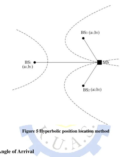
Figure 5 Hyperbolic position location method... 15

Figure 6 Angle of arrival method ... 16

Figure 7 Received signal strength indication method ... 17

Figure 8 The flow chart of the location tracking system... 19

Figure 9 Discrete-time nonlinear dynamic system... 21

Figure 10 Block diagram of the UT processing [Haykin, 2001] ... 23

Figure 11 Example of the UT for mean and covariance propagation [Haykin, 2001]... 23

Figure 12 Actual and predicted trajectories of MS (Case 1) ... 35

Figure 13 The estimation error of trajectory (Case 1) ... 35

Figure 14 Actual and predicted velocities for the x and y directions (Case 1)... 36

Figure 15 Velocity estimation error (Case 1)... 37

Figure 16 Actual and predicted accelerations for the x and y directions (Case 1) ... 37

Figure 17 Acceleration estimation error (Case 1) ... 38

(11)

Table 1 Simulation parameters... 31

Table 2 Actual and assumed initial states of the UKF for four simulation cases ... 32

(12)

CHAPTER 1 INTRODUCTION

In a wireless network, as mobile station (MS) move, segments of connections have

to be cut off and reestablished with a frequency that corresponds to the speed of the mobile. Meantime, data completeness in terms of cell sequence preservation, duplicate cell prevention, and cell loss avoidance has to be provided. Additionally, quality-of-service (QoS) guarantees must be maintained regardless of the MS’s mobility. When the wireless services become more pervasive and convenient, one of the key problems is the location tracking or location management (also known as mobility tracking or mobility management). Location tracking is the set of methods by which the system can locate a MS at any given time.

The location tracking approach is two folds： location update and location

prediction. Location update is a passive strategy which the network system regularly records the current location of the MS in database. Tracking algorithms depend on the location updating that is triggered based on network topology or MS’s call and mobility patterns. As a positive strategy in location prediction, the system proactively estimates the MS’s location based on a MS motion model. Location prediction capability depends on the precision of this model and the efficiency of the prediction algorithm.

Most of the recent studies have focused on the update method [Wong and Leung, 2001; Akyol and Cox, 1997], and relatively little attention has been given to the prediction side. Accurate prediction of a MS based on its previous location will improve the efficiency of location tracking. The task of location tracking and system resources

(13)

used will become substantially efficient if MS movement pattern is known in advance. Liu et al. (1998) proposed to use the extended Kalman filter (EKF) for tracking the mobility of a MS in wireless ATM network using the forward link received signal strengths indication (RSSI). Zaidi and Mark (2005) proposed a new mobility tracking algorithm based on RSSI measurement and EKF. It is well known that the EKF is based on linearization of the underlying nonlinear dynamic system, and often diverges when the system exhibits strong nonlinearity. In the most literatures, typically, their measurements are based on the time of arrival (TOA) or time difference of arrival (TDOA), angle of arrival (AOA) [Cong and Zhuang, 2002], and received signal strength (RSS) [Liu et al.,1998].

In order to accurately estimate the MS movement, the equation of motion can be modeled as a nonstationary process with dynamic states that are nonlinearly related to a time-correlated Gaussian process whose motion pattern behaves like a Markv process. Estimation of the model parameters is performed by means of the unscented Kalman filter (UKF). The UKF is a novel and effective estimate tool. It is used to resolve the nonlinear dynamics and measurement problems, and uses the measurements to compute the motion parameters, usually obtaining optimal MS movement estimations for real-time applications.

Julier and Uhlmann (1995; 1997) proposed the UKF as a derivative-free alternative to the EKF in the framework of state estimation. The UKF uses a deterministic sampling approach. The state parameters distribution are approximated by Gaussian random variable (GRV), but it used a minimal set of carefully chosen sigma points. When these sigma points propagated through any nonlinear system, the mean and

(14)

covariance of the GRV accurately approximated to the third-order. On the contrary, EKF only achieves first-order accuracy.

The UKF’s advantage is that it doesn’t use any linearization procedures. Therefore its covariance and Kalman gain estimates are more accurate, and leads to better state estimate. The UKF has been proposed and applied to various problems [Akin et al., 2003; Tak ea al., 2002; Mao et al., 2003; Li and Leung, 2003].

In this paper, we propose to employ the UKF to estimate the mobility information (location, velocity, and acceleration). We assume the mobility estimation is based on RSSI measurements at MS. We simulate four cases in this thesis. These cases respectively used different number of base stations in the measurement. Simulation results are provided to demonstrate the superiority of the proposed algorithm.

The remainders of this paper are organized as follows. In Chapter 2, we describe the nonlinear dynamic system model under consideration, and introduce the mathematical formulation for the problem of location tracking in wireless networks. In Chapter 3, we briefly introduce some background materials on trajectory prediction method. Chapter 4 describes the simulation results. Conclusion and future works are given in Chapter 5.

(15)

CHAPTER 2 FUNDAMENTAL CONCEPTS

This chapter develops the fundamental concepts as follows. Section 2.1 describes mobile station dynamic model. Section 2.2 depicts mobile station measurement equation.

2.1 Mobile Station Dynamic Model

The mobility model we present is along the lines of [Liu et al.,1998] to mimic

human movement behavior. The model is built of two terms： global mobility model (GMM) and local mobility model (LMM). The GMM is in terms of cells crossed by the mobile during the lifetime of the connection, and deterministic model is used to create intercell movements. The LMM resolution is in terms of a 3-component sample space (position, speed, direction) that varies with time. The rationale of having a local mobility model is based on the observation that the apparently random choice of intercell movement due to MS speed position and cell geometry. The MS mobility models found previously in literature assumed straight line movement or constant speed [Austin and Stuber, 1994； Viayan and Holtzman, 1993], which did not reflect reality. The LMM used in [Liu et al.,1998] assumes a random acceleration distribution with Gaussian assumptions during employment of Kalman filter as a state estimator.

(16)

2.1.1 Global Mobility Model

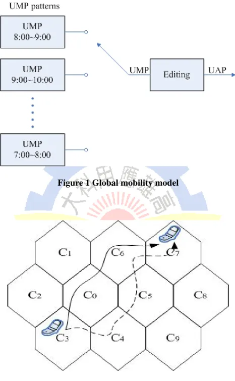
The global mobility model (GMM) is shown in Figure 1. It is motivated by the fact that most MS exhibit some regularity in their daily movement. This regularity can best be characterized by a number of MS mobility patterns (UMP’s), recorded in a database for each MS and indexed by the occurrence time. The UMP’s are like the movement patterns in [Tabbane, 1995； Liu and Maguire, 1995], but are more robust in the sense that we decrease the UMP’s sensitivity to small deviations from the MS’s actual path (UAP). The UMP is described by a cell

( )

c sequence _i

(

=c c_{1 2} c c c_i₋₁ _{i i}₊₁ c_n

)

, then we model the regular movement of a MS as an edited UMP by following operations：

1. inserting a cell ck at position i of the UMP makes up UAP： c c_{1 2} c c c c_i₋₁ _{k i i}₊₁ c_n,

2. deleting the cell ci at position i of the UMP makes up UAP： c c_{1 2} c c_i₋₁ _i₊₁ c_n,

3. changing a cell ci to another cell ck makes up UAP： c c_{1 2} c c c_i₋₁ _{k i}₊₁ c_n.

Figure 2 shows an example of a UMP , and its edited version UAP , which can be obtained by changing and inserting .

3 0 6 7

c c c c

3 4 5 6 7

(17)

Figure 1 Global mobility model

(18)

2.1.2 Local Mobility Model

In order to evolve time-varying movement patterns, we model a MS as a linear dynamic system driven by deterministic input command and random acceleration

shown in Figure 3. In real condition, the acceleration range for a MS can be rather wide. Furthermore, traffic lights and road turns can lead to abrupt changes in velocity. In order to produce such sudden and unexpected changes, while covering the wide acceleration range, is modeled as a semi-Markov process with a finite number of “state” as possible discrete levels of acceleration. A semi-Markov process includes the Markovian state transition probability and random service time in one state prior to switching to another state [Howard, 1964]. Random acceleration is modeled as a zero-mean Gaussian random variable with a variance that is chosen to cover the “gap” between adjacent acceleration states. Figure 4 shows the conditional distribution of given a different state level

( ) u t ( ) r t ( ) u t 1, , , 2 m l l l ( ) r t ( ) r t L=

{

l l1, ,2 ,lm

}

within the

acceleration range

[

−A_max, A_max

]

. Thus, the process takes values in the set . This approach to modeling acceleration has been applied to tracking maneuvering targets in tactical weapons systems [Singer, 1970 ； Moose and Vanlandingham, 1979].

( )

u t

= ×

(19)

Figure 3 Local mobility model

Figure 4 The conditional distribution of r t( )

2.1.3 Dynamical Equations for a Mobile Station

Based on the model described above, the dynamical equations are derived for

continuous-time movement, and are then transformed into discrete-time is according to the standard discretisatior procedure, thereby providing accurate statistical representation of the movement behavior.

It is known that in two-dimensional Cartesian coordinates, the movement can be

described by a first-order, vector differential equation [Brown and Hwang, 1997] with the MS state s t( ) at time t as follows:

(20)

s t( )= ⎡_⎣x t

( ) ( )

x t y t

( )

y t

( )

⎤_{⎦ (2.1)}Τ

where x t( ) and represent the position of the MS at time and the first-order derivatives of

( )

y t t

( )

x t and y t( ) specify the velocity.

The acceleration, a t( )=

[

x t( ) y t( )

]

Τ is modeled as follows：

a t( )=u t( )+r t( ) (2.2) where x t( ) and y t( ) specify the acceleration in the x and y directions in a two-dimensional grid, is the two-dimensional driving

command with and as independent Markov processes that take values

from a set of acceleration levels

( ) _x( ) _y( ) T u t = ⎣⎡u t u t ⎤⎦ ( ) x u t u t_y( )

{

1, , m

}

L= l l acting in the and directions,

respectively, and

x y

( ) _x( ) _y( )

r t = ⎣⎡r t r t ⎤⎦ is a zero-mean Gaussian process chosen to Τ

cover the gaps between adjacent levels of the process u t( ). Combining (2.1) and (2.2), we have：

s t

( )

=Fs t

( )

+Eu t

( )

+Gr t

( )

(2.3) where 0 0 i i F F F ⎡ ⎤ = ⎢ ⎣ ⎦⎥ 0 0 i i g E G g ⎡ ⎤ = = ⎢ ⎥ ⎣ ⎦ with 0 1 0 0 i F = ⎢⎡ ⎤ ⎣ ⎦⎥ 0 1 i g = ⎢ ⎥⎡ ⎤ ⎣ ⎦. The autocorrelation function of r t( ) is given by

(21)

where 2 1

σ is the common variance of r t_x( ) and r t_y( ), α is the reciprocal of the random acceleration time constant, and I is the k kk × identity matrix for any

positive integer . Such a random process can be obtained by passing the white Gaussian signals

k

( )

x

( )

y

( )

w t = ⎣⎡w t w t ⎤⎦ through a one-pole shaping filter, where Τ

and

( )

x

w t w t are uncorrelated _y

( )

r t

( )

= −αr t

( )

+w t

( )

. (2.5) The autocorrelation function of w t is given by

( )

R_w

( )

τ =2ασ δ τ₁2

( )

I₂ (2.6) where δ τ

( )

is the Dirac delta function.

Combining (2.3) and (2.4), the linear system describing the state evolution can be written as x( )t =A′x( )t +B′u( )t +C′w( )t (2.7) where x( )t =

[

x t( ) x t( ) x t( ) y t( ) y t( ) y t( )

]

T u( )t = ⎣⎡u t_x( ) u t_y( )⎤_⎦T w( )t = ⎣⎡w t_x( ) w t_y( )⎤_⎦T with

(22)

0 1 0 0 0 0 0 0 1 0 0 0 0 0 0 0 0 0 0 0 0 1 0 0 0 0 0 0 1 0 0 0 0 0 0 0 0 0 1 0 0 0 0 0 1 0 . 0 0 0 0 0 1 0 0 0 0 0 1 A B C α α ⎡ ⎤ ⎢ ⎥ ⎢ ⎥ ⎢ − ⎥ ′ = ⎢ ⎥ ⎢ ⎥ ⎢ ⎥ ⎢ ⎥ − ⎣ ⎦ ⎡ ⎤ ⎡ ⎤ ⎢ ⎥ ⎢ ⎥ ⎢ ⎥ ⎢ ⎥ ⎢ ⎥ ⎢ ⎥ ′=_⎢ _⎥ ′=_⎢ _⎥ ⎢ ⎥ ⎢ ⎥ ⎢ ⎥ ⎢ ⎥ ⎢ ⎥ ⎢ ⎥ ⎣ ⎦ ⎣ ⎦

By sampling the state every time units, the appropriate dynamic equation is given by T ( ) ( ) ( ) A T ( ) t T A t T t T A t T ( ) t t t T+ =e ′ t +

∫

+ e ′ + −τ B d′ τ+

∫

+ e ′ + −τ C τ τd x x ′w k (2.8)

where the corresponding discrete-time state equation is given by x_k₊₁ =A T( , )α x_k+B T( )u_k + w d . (2.9) it follows that ( ) ( ) ( , ) ( ) ( ) A T t T _{A t T} t t T A t T k _t A T e B T e B d e C τ τ α τ τ τ ′ + _{′ + −} + _{′ + −} = ′ = ′ =

∫

w w where

(23)

1 4 2 5 3 1 4 2 5 3 1 0 0 0 0 0 1 0 0 0 0 0 0 0 0 0 0 0 ( , ) ( ) 0 0 0 1 0 0 0 0 0 1 0 0 0 0 0 0 0 0 T p p p p p A T B T T p p p p p α ⎡ ⎤ ⎡ ⎤ ⎢ ⎥ ⎢ ⎥ ⎢ ⎥ ⎢ ⎥ ⎢ ⎥ ⎢ ⎥ =_⎢ _⎥ =_⎢ _⎥ ⎢ ⎥ ⎢ ⎥ ⎢ ⎥ ⎢ ⎥ ⎢ ⎥ ⎢ ⎥ ⎢ ⎥ _⎣ _⎦ ⎣ ⎦ _k (n 1)T

[

( 1)

]

( ) nT A n T τ C τ τd + ′ =

∫

+ − w w (2.10) where 1 2 2 3 4 5 1 ( 1 ) 1 (1 ) 1 1 . T T T T T p T p e p e p T e p e α α α α α α − − − − − = − + + = − = = − + = − e

Since w( )t is a white noise, E

[

w w_k _{k i}₊

]

=0 for (i≠0) , so that is a discrete-time white noise sequence. The covariance matrix of is given by

k w Q w_k

[ ]

{

[ ] [ ]

(

)

}

11 12 13 21 22 23 31 32 33 2 1 11 12 13 21 22 23 31 32 33 0 0 0 0 0 0 0 0 0 2 0 0 0 0 0 0 0 0 0 T Q k E k k q q q q q q q q q q q q q q q q q q ασ = ⎡ ⎤ ⎢ ⎥ ⎢ ⎥ ⎢ ⎥ = _⎢ _⎥ ⎢ ⎥ ⎢ ⎥ ⎢ ⎥ ⎢ ⎥ ⎣ ⎦ w w (2.11) where

(24)

(

)

(

)

(

)

(

)

(

)

3 3 2 2 2 11 5 2 2 12 4 2 13 3 2 22 3 2 23 2 2 33 1 2 1 2 2 4 2 3 1 1 2 2 2 2 1 1 2 2 1 4 3 2 2 1 1 2 2 1 1 2 T T T T T T T T T T T T T q e T T T q e e Te T T q e Te q e e T q e e q e α α α α α α α α α α α α α α α α α α α α α α α α α α 2 e α − − − − − − − − − − − − ⎛ ⎞ = _⎜ − + + − − _⎟ ⎝ ⎠ = + − + − + = − − = − − + = + − = − and q_ij =q_ji, i≠ j .

2.2 Mobile Station Measurement Equation

In wireless cellular networks, some new features such as dedicated reverse-link for each MS, adaptive antenna array for angle of arrival (AOA) estimation, and forward link common broadcasting channel, are used to measurement that avail in practice for mobile tracking. Some measurement scenarios are discussed hereafter.

2.2.1 Time Difference of Arrival

First of all, methods for determining the time difference of arrival (TDOA) from the spread-spectrum signal, including the coarse timing acquisition with a sliding correlator or matched filter and fine timing acquisition with a delay-locked loop (DLL) or tau-dither loop (TDL) [Ziermer and Peterson, 1985； Viterbi, 1999]. Time delay estimation is used to find the TDOA of acknowledgement signals from MS to BSs that are determined. This TDOA estimate is used to calculate the range difference

(25)

measurements between the base stations. This method is also sometimes called hyperbolic position location method, as shown in Figure 5. TDOA can be estimated by two methods：

1. Subtracting the TOA measurements from the two corresponding BSs, 2. Correlating two versions of the acknowledgement signal at the two BSs,

The second method, commonly known as Generalized Cross-Correlation (GCC) method [Knapp and Carter, 1976], is more robust and will be adopted for the rest of this thesis. The model is given by

_{k i}_, 1

(

D_{k i}_, D_k_,1

)

n_{k i}_,, i 2, 3

c

τ

τ = − + = (2.12) where 8 is the speed of light；

3 10

c= × nk i, ~ 0,

(

2

)

τ

σ is the measurement noise of

TDOA with zero mean and covariance σ between the _τ2 BS and the home BS； and th i

(

) (

2

)

1₂ , k i k i k i

D =⎡_⎣ x −a + y −b 2⎤_{⎦ is the distance between the mobile and base station}

of cell , which can be further expressed in terms of the mobile’s position i

(

x y_k, _k

)

at time k and the location of base station

(

a b . _i, _i

)

(26)

Figure 5 Hyperbolic position location method

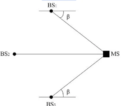
2.2.2 Angle of Arrival

The second way, with multiple antennas to collect the radio signal at the base station, we could apply array signal processing algorithms [Krim and Viberg, 1996] to estimate the AOA. The AOA method utilizes multi-array antennas and tries to estimate the direction of arrival of the signal of interest. The AOA method is sometimes called direction of arrival (DOA) method. Thus a single DOA measurement restricts the MS location along a line in the estimated DOA. If at least two such DOA estimates are available from two antennas at two different locations, the position of the signal source can be located at the intersection of the lines of bearings from the two antennas. Usually

(27)

multiple DOA estimates are used to improve the estimation accuracy by using the redundant information. Figure 6 shows the method where the MS location is found by the intersection of DOA of the signal for three antenna arrays. The model is given by

_, tan( )1 k i _,, 1, 2, 3 k i k i k i y b n i x a β β ₌ − ⎛ − ⎞₊ ⎜ ₋ ⎟ ⎝ ⎠ =

(

2

)

, ~ 0, k i nβ N (2.13)

where σ is the estimation error of AOA at the _β ith BS, and

(

2

)

0,

N σ _β stands for the normal distribution with zero mean and covariance σ_β2.

Figure 6 Angle of arrival method

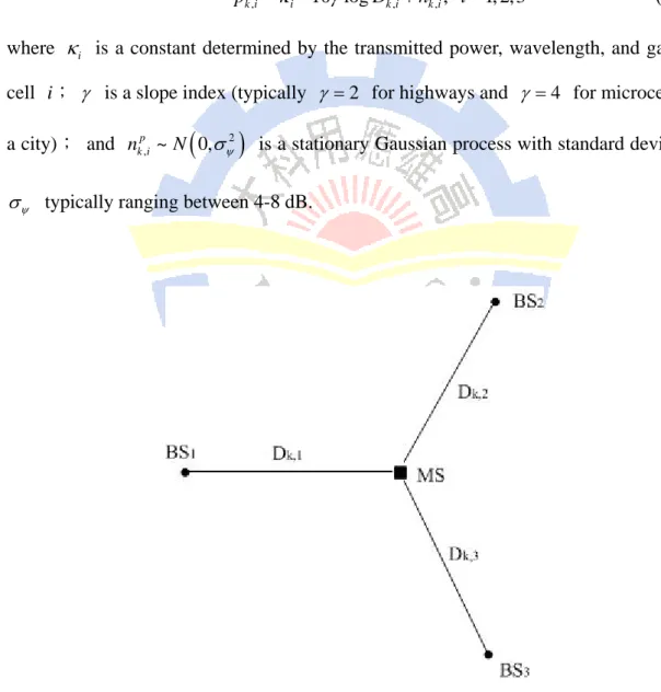
2.2.3 Received Signal Strength Indication

Finally, the Received Signal Strength Indication (RSSI) in wireless cellular networks contains the distance information between a MS and a given BS. Measured in

(28)

decibels at the mobile station, RSSI can be modeled as the sum of two terms： one due to path loss, and another due to shadow fading. Fast fading is neglected assuming that a low-pass filter is used to attenuate Rayleigh or Rician fade. Therefore, the RSSI received at the MS, shown in Figure 7, from the base station at time can be formulated as [Xia, 1996]

k

p_{k i}_, = −κ_i 10 logγ D_{k i}_, +n_{k i}p_,, i=1, 2, 3 (2.14) where is a constant determined by the transmitted power, wavelength, and gain of cell i；

i κ

γ is a slope index (typically γ =2 for highways and γ =4 for microcells in a city)； and n_{k i}p_, ~N

(

0,σ is a stationary Gaussian process with standard deviation _ψ2

)

ψ

σ typically ranging between 4-8 dB.

(29)

CHAPTER 3 LOCATION TRACKING AND

TRAJECTORY PREDICTION METHOD

In this chapter, an unscented Kalman filtering (UKF) is introduced for MS state estimations in the wireless cellular networks. The MS state model can capture a wide range of mobility scenarios, including sudden stop and changes in acceleration. In the measurement segment, the RSSI is used to compute the motion parameters to give optimal MS movement estimations for real-time applications.

The flow chart of the location tracking system is shown in Figure 8. It shows the basic operations involved in the MS state estimation problem. In section 3.1, a more detail description about estimation method is discussed. Section 3.2 presents the mathematical formulations between the state parameters and the RSSI measurements.

(30)

(31)

3.1 Estimation Method

The filtering problem of interest in this thesis is to find the best (in the sense of minimum mean square error (MMSE)) linear estimate of the state vectors of the MS, which evolves according to the discrete time nonlinear transition equation [Gelb, 1974； Julier et al., 1995]

xk

x_k₊₁ = f

(

x , u_k _k

)

+G w_k _k (3.1) y_k =h

( )

x_k + (3.2) v_k

where any time instant is denoted by subscript . is the state of the mobile unit at sampling instant ; is the deterministic matrix mapping the process noise into state space, and is the additive white process noise representing modeling errors. is the observation vector which is related to the state vector of the mobile station at sampling instant , and is the additive white measurement noise.

k x_k k Gk k w yk k vk f i and

( )

h i

( )

are the nonlinear process and measurement model. It is also assumed that the process noise and the measurement noise are zero mean and uncorrelated white sequences for all sampling instants , and their corresponding covariance and cross covariance are k w vk k E G w w G⎡_⎣ _k _k _jT _kT_⎦⎤=G E w w_k _⎣⎡ _k _jT⎤_⎦G_kT =δ_kjG_kQ_kG_kT (3.3) T k j kj k E v v⎡_⎣ ⎤ =_⎦ δ R (3.4) 0 , T k j E v w⎡_⎣ ⎤ =_⎦ ∀k j (3.5) where δ is the delta function that, by definition, is zero except _kj k= j. E i

[ ]

denotes

(32)

the excepted value operation. The block diagram of the proposed system is shown in Figure 9.

Because the true state vectors of the MS are not known, they must be estimated, and we begin with introducing the UKF to estimate the states of the MS； the state assignment is presented in section 3.2.

k

x

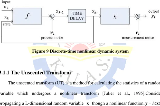
Figure 9 Discrete-time nonlinear dynamic system

3.1.1 The Unscented Transform

The unscented transform (UT) is a method for calculating the statistics of a random variable which undergoes a nonlinear transform [Julier et al., 1995].Consider propagating a L-dimensional random variable though a nonlinear function, . Assume has mean

x y=h( )x

x x and covariance . In order to calculate the statistics of , the UT creates sigma point vectors

x

P

( )

h

=

y x χ_i with dimension 2L+1 according to the followings: 0 ( ) 1,..., ( ) 1,..., 2 i i i i L i L i L L χ χ η χ η ₋ = = + = = − = + x x x x P x P (3.6)

(33)

where η= (L+λ) and λ=L(α2−1) are scaling parameters. The constant α determines the spread of the sigma points around x and is usually set to a small positive value; β is used to incorporate prior knowledge of the distribution of (for Gaussian distributions,

x 2

β = is optimal). ( P_x)_i

L

is the row or column of the matrix square root of .

th

i

x

P

When given these set of sigma vectors, the approximation process is as given below,

1. Each sigma vector is propagated through the nonlinear function h. ( ) 0,..., 2

i h i i

ζ = χ = (3.7) 2. The mean and covariance for y are approximated using a weighted sample

mean and covariance of the posterior sigma vectors ζi,

2 ( ) 0 2 ( ) 0 ( )( ) i L m i i i i L c T i i i i W W ζ ζ ζ = = = = = = −

∑

y y P y −y . (3.8)

with weights W_i given by

( ) 0 ( ) ( ) 2 0 0 ( ) ( ) ( ) 0 ( ) (1 ) 1,..., 2 . 2 m c m m m c i i W L W W W W W i L λ λ α β λ = + = + − + = = = (3.9)

(34)

Figure 10 Block diagram of the UT processing [Haykin, 2001]

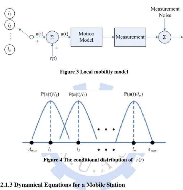
A simple example is shown in Figure 11 [Haykin, 2001] for a two-dimensional system： (a) shows the true mean and covariance propagation using Monte-Carlo sampling method； (b) shows the results using a linearization approach (EKF)； and (c) shows the performance of the UT (note that only 5 sigma points are required).

Figure 11 Example of the UT for mean and covariance propagation [Haykin, 2001]. (a) The true mean and covariance using real sampling process,

(35)

3.1.2 The Unscented Kalman Filter

The UKF is an extension of UT to the Kalman Filter framework [Van Der Merwe and Wan, 2001; Tak et al., 2002], and it uses the UT to implement the transformations for both nonlinear process (time update or prediction) and sensor models (measurement update or correction).

The Standard UKF algorithm is shown as follows: 1. Initialize the state mean and covariance matrix:

[ ]

0 E 0 0 ( 0 0)( 0 0) T E ∧ _⎡ ∧ ∧ _⎤ = = _⎢ − − _⎥ ⎣ ⎦ x x P x x x x (3.10) for k∈

{

1,...,∞ .

}

2. Calculate sigma points χ_{i k}_, ₋₁ using equation (3.6). 3. Time update equations (Prediction):

(

)

, 1 , 1 2 ( ) , 1 0 2 ( ) , 1 , 1 0 , 1 , 1 2 ( ) , 1 0 ( ) ( )( ) i k i k k L m k _i _{i k k} i L c k k k i i k k i k k i i k k i k k L m i k i k k i f W W h W T k ζ χ ζ ζ ζ δ ζ δ − − − ∧ − = − − ∧ ∧ − − − = − − − ∧ − = = = = − − = =

∑

x P x x y + Q (3.11)

where the optimal prediction (i.e., prior mean) of x_k is written as k

− ∧

x

(similar interpretation for the optimal prediction _k

− ∧ y )； = process noise covariance matrix. k Q , 1 i k k

ζ ₋ , i=0,1,..., 2L are the computed sigma points by equation (3.11); the prediction of the state variable (output) at time instant k

(36)

based on the state variable (input) at time instant k− is denoted by subscript 1 1

k k− .

4. Measurement update equations (Correction):

~ ~ ~ ~ ~ ~ ~ ~ ~ ~ 2 ( ) , 1 , 1 0 2 ( ) , 1 , 1 0 1 ( )( ) ( )( ) ( ) k k k k k k k k k k L c T i i k k k i k k k k y y _i L c T k i i k k i k k k x y _i k x y y y k k _k _k _k T k k k k y y W W K K y K K δ δ ζ δ − − ∧ ∧ − − = − − ∧ ∧ − − = − − − ∧ ∧ ∧ − = − − = − − = = + − = −

∑

P y y +R P x P P x x y P P P y (3.12) where

: measurement noise covariance matrix

k

R

: measurement correlation matrix

~ ~ k k y y P : cross-correlation matrix ~ ~ k k x y P : Kalman gain k K : updated state k ∧ x

: update state covariance matrix

k P : current measurement. k y

3.2 State Assignment

An approximated dynamic model is considered based on the assumption that the motion is to mimic human movement behavior model that described in formula 2.9 and

(37)

given by 1 1 1 1 1 4 1 2 5 3 1 1 2 5 3 v a v v a a a v a v _v _a a _a k k k k k k k k k k k k _k _k _k k _k _k k x x x k x x x x x x x k k k y y y _y _y _y y _y _y 4 k k y x T p p u x p p u p W y y T p p u p p u p W + + + + + + + + + ⎡ ⎤ ⎡ ⎤ ⎢ ⎥ ⎢ ⎥ ₊ ₊ ⎢ ⎥ ⎢ ⎥ ⎢ ⎥ ⎢ ⎥ ₊ ⎢ ⎥ ⎢ ⎥ = _{= ⎢} _⎥ + + + ⎢ ⎥ ⎢ ⎥ ⎢ ⎥ + + ⎢ ⎥ ⎢ ⎥ ⎢ ⎥ ⎢ ⎥ ₊ ⎣ ⎦ ⎢_⎣ ⎥_⎦ x

where and represent the position, and their first-order vector derivatives of and represent the relative speed； and a denote the two-dimensional random acceleration vector； and denote the driving command. T is the sampling time interval. In addition, the parameters

x y v_x v_y ax y x u u_y , 1, 2, , 5 i

p i= have been described in the section 2.1.3.

3.2.1 Process (Dynamic) Model

The discrete time dynamic model can be written as x_k₊₁ =Ax_k+Bu_k+Gw_k

where A is a 6-by-6 and B is a 6-by-2 block diagonal matrix

1 4 2 5 3 1 4 2 5 3 1 0 0 0 0 0 1 0 0 0 0 0 0 0 0 0 0 0 0 0 0 1 0 0 0 0 0 1 0 0 0 0 0 0 0 0 T p p p p p A B T p p p p p ⎡ ⎤ ⎡ ⎤ ⎢ ⎥ ⎢ ⎥ ⎢ ⎥ ⎢ ⎥ ⎢ ⎥ ⎢ ⎥ =_⎢ _⎥ =_⎢ _⎥ ⎢ ⎥ ⎢ ⎥ ⎢ ⎥ ⎢ ⎥ ⎢ ⎥ ⎢ ⎥ ⎢ ⎥ _⎣ _⎦ ⎣ ⎦ where

(38)

1 2 2 3 4 5 1 ( 1 ) 1 (1 ) 1 1 T T T T T p T p e p e p T e p e α α α α α α − − − − − = − + + = − = = − + = − e

3.2.2 Measurement (Sensor) Model

In this thesis, we used the RRSI in the measurement model. The RSSI, measured in dB, received at the mobile unit site, emitted from the base station. Denote the measurements at time instance as that is a 4-by-1 matrix. Then, we have the following measurement equation

k zk

z_k =h

( )

x_k + v_k

where v_k = ⎣⎡n_k_,1,n_k_,2,n_k_,3,n_k_,4⎤⎦Τ with covariance matrix I and 3, 4

2 4

R=σ_ψ

h_i

( )

x_k = −κ_i 10 logγ D_{k i}_,, i=1, 2,

where κi is a constant associated with transmitted power； γ is a slope index； and

(

) (

2

)

2 1₂ ,

k i k i k i

D =⎡_⎣ x −a + y −b ⎤_{⎦ is the distance between the mobile unit location}

(39)

2 2 10 m/s , 10 m/s

CHAPTER 4 SIMULATION RESULTS

We estimate those parameters including MS’s position, velocity, and acceleration. The simulation was implemented by using Matlab ver. 7.0.

To examine the performance of the UKF in the wireless cellular networks, simulations are carried out for the networks. No constraints are imposed, and the MS is permitted to move anywhere in the network along random trajectories with nonconstant speed. The dynamics are based on the movement model discussed in Section 2.1.3, except that the acceleration is present so that a known trajectory can be achieved for the purpose of performance tests. Simulation parameters are summarized in Table 1. In order to include the range of dynamic acceleration ⎡_⎣− ⎤_⎦

)

, five levels of

accelerations are selected as the states values of the

deterministic driving input. This set of acceleration levels is capable of generating a wide range of dynamic motion. The sampling interval is . The total duration of each sample is , which corresponds to 1 minute. The transition probability matrix

(

−7.5, 2.5, 0, 2.5, 7.5− 2 m/s T 0.1 s 600 N =

A is initialized as follows. The diagonal elements of A are set to zero and the off- diagonal elements in each row are initialized to a common value of 1/ 24.

The UKF coefficients are chosen as L= , 6 α =0.01, and β =2. The sampling time interval is t=0.1sec. The measurement noise covariance matrix has been set to

R =σ_ψI_i for ( ), where is an -by-i identity matrix. The process noise covariance matrix has been listed in formula 2.11. The choice of the matrix will

1, 2, 3

i= I_i i

(40)

(

0, 0

)

affect the accuracy of UKF estimates. These actual and assumed initial states of the UKF are listed in the Table 2. These four kinds of simulation cases are elaborately described as follows.

Case 1： One BS is used for the measurement.

In this case, we use only one BS in the networks. The BS is located at the coordinate . The true initial coordinate of the MS is

(

0, 0 . We assumed initial

)

coordinate of the MS is . The simulation results are shown in follows. The

actual and predicted trajectories of MS are plotted in Figure 12. The estimation error of trajectory is shown in Figure 13. Figure 14 shows the actual and predicted velocity for the x and y directions. Figure 15 draws the velocities estimation error. Figure 16 illustrates the actual and predicted accelerations for the x and y directions. Figure 17 shows the acceleration estimation error. In this case, we can conclude that estimation errors arise when we introduce use one BS in measurement process.

(

15, 10

)

Case 2： Two BSs are used for the measurement.

In this case, we use the two BSs in the networks. The BSs are located at the coordinates and . The true initial coordinate of the MS is

. We assumed initial coordinate of the MS is

(

30, 30

(

−30, 30−

(

0, 0

(

15, 10 . The simulation results are

)

shown as follows. The actual and predicted trajectories of MS are plotted in Figure 18. The estimation error of trajectory is shown in Figure 19. Figure 20 shows the actual and

(41)

predicted velocities for the x and y directions. Figure 21 draws the velocity estimation error. Figure 22 illustrates the actual and predicted accelerations for the x and y directions. Figure 23 shows the acceleration estimation error. In this case, the tracking performance is better than those in case 1. Although the estimation error is decreasing, the convergence speed is still slow.

Case 3： Three BSs are used for the measurement.

In this case, we use the three BSs in the networks. The BSs are located at the coordinates

(

30, 30

)

,

(

−30, 30

)

, and

(

0, 30−

)

. The true initial coordinate of the MS is

(

0, 0

)

. We assumed initial coordinate of the MS is

(

15, 10 . The simulation

)

results are shown as follows. The actual and predicted trajectories of MS are plotted in Figure 24. The estimation error of trajectory is shown in Figure 25. Figure 26 shows the actual and predicted velocities for the x and y directions. Figure 27 draws the velocity estimation error. Figure 28 illustrates the actual and predicted accelerations for the x and y directions. Figure 29 shows the acceleration estimation error. In this case, the tracking condition and estimation error are significantly improved compared to those in one and two BSs case. But the estimation performance is not very satisfactory.

Case 4：Four BSs are used for the measurement.

In this case, we use the four BSs in the networks. The BSs are located at the coordinates

(

30, 30

)

,

(

−30, 30

)

,

(

30, 30−

)

, and

(

−30, 30−

)

. The true initial

(42)

coordinate of the MS is . We assumed initial coordinate of the MS is .

The actual and predicted trajectories of MS are plotted in Figure 30. The estimation error of trajectory is shown in Figure 31. Figure 32 shows the actual and predicted velocities for the x and y directions. Figure 33 draws the velocity estimation error. Figure 34 illustrates the actual and predicted accelerations for the x and y directions. Figure 35 shows the acceleration estimation error. Case 4 is the best result among four cases. Even the assumed initial coordinate of the MS deviates from the true one greatly, accurate tracking can also be achieved. That is to say, the accuracy of estimation MS state parameters will increase.

(

0, 0

)

(

50, 30

)

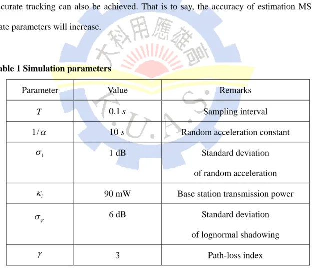
Table 1 Simulation parameters

Parameter Value Remarks

T 0.1 s Sampling interval

1/α 10 s Random acceleration constant

1

σ 1 dB Standard deviation

of random acceleration

i

κ 90 mW Base station transmission power

ψ

σ 6 dB Standard deviation

of lognormal shadowing

(43)

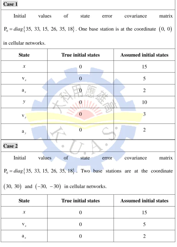
Table 2 Actual and assumed initial states of the UKF for four simulation cases Case 1

Initial values of state error covariance matrix

{

}

0

P =diag 35, 33, 15, 26, 35, 18 . One base station is at the coordinate

in cellular networks.

(

0, 0

)

State True initial states Assumed initial states

x 0 15 v_x 0 5 a_x 0 2 y _{0 10} vy 0 3 a_y 0 2 Case 2

{

}

0

P =diag 35, 33, 15, 26, 35, 18 . Two base stations are at the coordinate

and

(

30, 30

)

(

−30, 30−

)

x 0 15

v_x 0 5

(44)

y _{0 10}

vy 0 3

a_y 0 2

Case 3

{

}

0

P =diag 35, 33, 15, 26, 35, 18 . Three base stations are at the coordinate

, , and

(

30, 30

)

(

−30, 30

)

(

0, 30−

)

x 0 15 v_x 0 5 a_x 0 2 y _{0 10} v_y 0 3 a_y 0 2 Case 4

{

}

0

P =diag 35, 33, 15, 26, 35, 18 . Four base stations are at the coordinate

, ,

(

30, 30

)

(

−30, 30

)

(

30, 30−

)

, and

(

−30, 30−

)

(45)

x 0 50 v_x 0 10 a_x 0 2 y _{0 30} v_y 0 13 a_y 0 2

(46)

Figure 12 Actual and predicted trajectories of MS (Case 1)

(47)

(48)

Figure 15 Velocity estimation error (Case 1)

(49)

(50)

(51)

(52)

(53)

(54)

(55)

(56)

(57)

(58)

(59)

(60)

(61)

(62)

CHAPTER 5 CONCLUSIONS AND FUTURE WORKS

In this thesis, we have proposed a scheme for mobility estimation and prediction for the wireless cellular networks consisting of BS and MS. This research was motivated by importance of effective location management in a wireless cellular network. The location algorithm combines UKF for state estimation with an algorithm for estimating the parameters of a hidden Markov model that characterizes the acceleration behavior of the MS. Basically, we need RSSI measurements from BS. Four simulation cases are discussed for estimating the states from UKF processing.

Simulation results show that the UKF has an excellent mobility tracking and parameter estimation performance. It is evident from our results, four BSs measurement can successfully be used for tracking the MS in the wireless cellular networks. The trajectory error between the true and the estimated one is within 6 meters. The proposed location tracking technique can be applied in a variety of scenarios such as the provisioning of location-aware services.

This thesis has accomplished MS state parameters estimations, and future work will use the neural networks to train acceleration levels or demonstrate the performance comparisons of UKF and Particle filter.

(63)

REFERENCES

[Akyol and Cox, 1997]

Akyol, B.A. and Cox, D.C., “Signaling Alternatives in a Wireless ATM,” IEEE

Journal on Selected Areas in Communications, Vol. 16, pp. 35-49, January 1997.

[Akin et al., 2003]

Akin, B., Orguner, U., and Ersak, A., “State Estimation of Induction Motor Using Unscented Kalman Filter,” Proceedings of the 2003 IEEE Conference on

Control Applications, pp.915–919, June 2003.

[Austin and Stuber, 1994]

Austin, M.D. and Stuber, G.L., “Velocity Adaptive Handoff Algorithm for Microcellular System,” IEEE Transactions on Vehical Technology, Vol. 43, pp.549-561, August 1994.

[Brown and Hwang, 1997]

Brown, R.G. and Hwang, P.Y.C., Introduction to Random Signals and Applied

Kalman Filtering, 3rd ed., Wiley, New York, 1997. [Cong and Zhuang, 2002]

Cong, L. and Zhuang, W., “Hybrid TDOA/AOA Mobile User Location for Wideband CDMA Cellular System,” IEEE Transactions Wireless Communication, Vol. 1, No. 3, pp. 439-447, July 2002.

[Gelb, 1974]

Gelb, A., Applied Optimal Estimation, M.I.T. Press, Cambridge, Massachusetts,

(64)

[Haykin, 2001]

Haykin, S., Kalman Filtering and Neural Networks, John Wiley, New York,

2001. [Howard, 1964]

Howard, R.A., “System Analysis of Semi-Markov Process,” IEEE Trans. Mil.

Electron., Vol. MIL-8, pp.114-124, April 1964.

[Julier et al., 1995]

Julier, S.J., Uhlmann, J.K., and Durrant-Whyte, H., “A New Approach for Filtering Nonlinear Systems,” Proceedings of the American Control Conference, pp.1628–1632, 1995.

[Krim and Viberg, 1996]

Krim, H. and Viberg, M., “Two Decades of Array Signal Processing Research ： The Parametric Approach,” IEEE Signal Processing Magazine, Vol. 13, No. 4, pp. 67-94, 1996.

[Knapp and Carter, 1976]

Knapp, C.H. and Carter, G.C., “The Generalized Correlation Method for Estimation of Time Delay,” IEEE Transaction on Acoustics, Speech and Signal

Processing, Vol. ASSP-24, No. 4, pp. 320-327, August 1976.

[Li and Leung, 2003]

Li, W. and Leung, H., “Constrained Unscented Kalman Filter Based Fusion of GPS/INS/Digital Map for Vehicle Localization,” Proceedings of the 2003 IEEE

Intelligent Transportation Systems, Vol. 2, pp.1362–1367, 2003.

(65)

Liu, T., Bahl, P. and Chlamtac I., “Mobility Modeling, Location Tracking, and Trajectory Prediction in Wireless ATM Networks,” IEEE Journal on Selected

Areas in Communications, Vol. 16, No. 6, pp.922-936, August 1998.

[Liu and Maguire, 1995]

Liu, G.Y. and Maguire, G.Q., Jr., “A Predictive Mobility Management Algorithm for Wireless Mobile Computation and Communication,” Proc. IEEE Int. Conf.

Universal Personal Communication, 1995.

[Mao et al., 2003]

Mao, X., Wada, M., and Hashimoto, H., “Nonlinear GPS Models for Position Estimate using Low-cost GPS Receiver,” Proceedings of the IEEE Intelligent

Transportation Systems, October 2003.

[Moose and Vanlandingham, 1979]

Moose, R.L. and Vanlandingham, H.F., “Modeling and Estimation for Tracking Maneuvering Targets,” IEEE Transactions Aerospace and Electronic System, Vol. 15, No. 3, pp. 448-456, May 1979.

[Singer, 1970]

Singer, R.A., “Estimating Optical Tracking Filter Performance for Manned Maneuvering Targets,” IEEE Transactions Aerospace and Electronic System, 1970. [Tabbane, 1995]

Tabbane, S., “An Alternative Strategy for Location Tracking,” IEEE Journal on

Selected Areas in Communications, Vol. 13, No. 5, pp. 880-892, June 1995.

[Tak et al., 2002]

(66)

Constraints Solver,” Proceedings of the Computer Animation, 2002.

[Van Der Merwe and Wan, 2001]

Van Der Merwe, R. and Wan, E. A., “The Square-Root Unscented Kalman Filter for State and Parameter Estimation,” Proceedings of the IEEE International

Conference on Acoustics, Speech, and Signal Processing, pp.3461–3464, Salt Lake

City, Utah, May 2001. [Viayan and Holtzman, 1993]

Viayan, R. and Holtzman, J.M., “A Model for Analyzing Handoff Algorithms,”

IEEE Transactions on Vehical Technology, Vol. 42, pp. 351-356, August 1993.

[Viterbi, 1999]

Viterbi, A.J., CDMA：Principles of Spread Spectrum Communications, 4th edition, Addison-Wesley Reading, Mass., USA, 1999.

[Wong and Leung, 2001]

Wong, W.S.V. and Leung, C.M.V., “An Adaptive Distance-based Location Update Algorithm for Next-generation PCS Networks,” IEEE Tournal on Selected Areas in

Communications, Vol. 19, No. 10, pp.1942-1952, October 2001.

[Xia, 1996]

Xia, H.H., “An Analytical Model for Predicting Path Loss in Urban and Suburban Environments,” Proc. PIRMC, 1996.

[Zaidi and Mark]

Zaidi, Z.R. and Mark, B.L., “Real-Time Mobility Tracking Algorithms for Cellular Networks Based on Kalman Filtering,” IEEE Transactions on Mobile Computing, Vol. 4, No. 2, pp. 195-208, March/April 2005.

(67)

[Ziermer and Peterson, 1985]

Ziermer, R.E. and Peterson, R.L., Digital Communications and Spred Spectrum

利用非察覺型卡門濾波器理論進行無線細胞網路之即時位置追蹤

國 立 高 雄 應 用 科 技 大 學

電 機 工 程 系

碩 士 論 文

利用非察覺型卡門濾波器理論進行無線細胞網路

之即時位置追蹤

REAL-TIME LOCATION TRACKING FOR WIRELESS

CELLULAR NETWORKS USING UNSCENTED

KALMAN FILTER

研 究 生：潘 政 宏

指導教授：王 冠 智

National Kaohsiung University of Applied Sciences

REAL-TIME LOCATIOON TRACKING FOR

WIRELESS CELLULAR NETWORKS USING

UNSCENTED KALMAN FILTER

by

C.H. Pan

Advised by

Luke K. Wang

A Thesis

Submitted to

Institute of Electrical Engineering

in Partial Fulfillment of the Requirements

for the Degree of Master

in

Electrical Engineering

Kaohsiung, Taiwan, Republic of China

June 2006

Real-time Location Tracking for Wireless Cellular Networks Using

Unscented Kalman Filter

Institute of Electrical and Control Engineering

National Kaohsiung University of Applied Sciences

ABSTRACT

利用非察覺型卡門濾波器理論

進行無線細胞網路之即時位置追蹤

國立高雄應用科技大學 電機工程系 碩士班

摘 要

誌 謝

CONTENTS

LIST OF FIGURES AND TABLES

CHAPTER 1

INTRODUCTION

CHAPTER 2

FUNDAMENTAL CONCEPTS

2.1 Mobile Station Dynamic Model

2.1.1 Global Mobility Model

( )

(

)

2.1.2 Local Mobility Model

{

}

[

]

2.1.3 Dynamical Equations for a Mobile Station

( ) ( )

( )

( )

[

]

{

}

( )

( )

( )

( )

( )

( )

( )

( )

( )

( )

( )

( )

( )

( )

( )

( )

[

]

國立高雄應用科技大學

電機工程系

碩士論文

研究生：潘政宏

指導教授：王冠智

國立高雄應用科技大學電機工程系碩士班

摘要

誌謝