Multi-Rate Throughput Optimization for Wireless
Local Area Network Anomaly Problem
Yu-Liang Kuo
∗, Kun-Wei Lai
†, Frank Yeong-Sung Lin
†, Yean-Fu Wen
†, Eric Hsiao-Kuang Wu
‡, Gen-Huey Chen
∗∗
Dept. of Computer Science and Information Engineering, National Taiwan University
†Dept. of Information Management, National Taiwan University
‡Dept. of Computer Science and Information Engineering, National Central University
Abstract— Due to varying wireless channel conditions, the IEEE 802.11 wireless local area network (WLAN) standard supports multiple modulation types to accommodate the tradeoff between data rate and bit error rate. In [9], Heusse, Rousseau, Berger-Sabbatel and Duda theoretically analyzed a performance anomaly when multi-rate stations with different modulation types exist in IEEE 802.11 WLANs. The performance anomaly is: the aggregate throughput of those stations transmitting at a higher data rate will dramatically degrade below the same level as that of those stations transmitting at a lower data rate. In this paper, we address the anomaly problem and formulate a nonlinear mixed integer programming problem to maximize the total aggregate throughput of all stations subject to that the channel occupancy times among the stations transmitting at different data rates are kept at a fairness ratio. With its aid, a single-hop WLAN can dynamically accommodate the resource access usage to maximize the system throughput in varying fading environments. We prove that the optimization problem is intractable and propose a heuristic solution based on a penalty function with gradient-based approach to solve it. We show the effectiveness of the approach via computational experiments and provide some useful guidelines to regulate the parameters needed for the approach.
I. INTRODUCTION
Wireless local area networks (WLANs) have been receiving a lot of attention during the last few years due to the extensive development of WLAN standards. For example, IEEE 802.11 [2] is widely adopted in many types of hot spots and has been becoming the de facto WLAN standard in recent years. Later, the IEEE 802.11b [4] and 802.11a/g [3], [5] standards further enhance the IEEE 802.11 physical layer protocol to support maximum data rate up to 11 Mbps and 54 Mbps, respectively. Higher data rates are usually achieved by more efficient modulation types. Modulation is the process of translating a data stream into a form suitable for transmitting on the physical medium. The performance criterion of a modulation type is often measured by its ability to preserve the accuracy of transmitted bits over wireless channels. As a symbol is transmitted with a small number of encoded bits (i.e., with a high data rate) under a low quality channel condition, it will be hard to decode the received signal. In other words, when the data is transmitted at a higher data rate, it will suffer from a higher bit error rate.
In the IEEE 802.11b standard, four modulation types whose data rates are 11 Mbps, 5.5 Mbps, 2 Mbps, and 1 Mbps, re-spectively, are supported to accommodate the tradeoff between
data rate and bit error rate in different fading environments. Heusse, Rousseau, Berger-Sabbatel and Duda [9] theoretically analyzed a performance anomaly when multi-rate traffic is supported in IEEE 802.11b WLAN. The performance anomaly is: the aggregate throughput of those stations transmitting at a higher data rate dramatically degrades below the same level as that of those stations transmitting at a lower data rate. The performance anomaly arises because the basic CSMA/CA channel access method guarantees that the long-term channel access probabilities of the stations transmitting at different data rates are the same. Hence the long-term channel occupancy time for those stations transmitting at a lower data rate will be larger than those stations transmitting at a higher rate. When one station transmitting at a lower data rate captures the channel, it will last for a longer time and hence penalize the aggregate throughput of those stations transmitting at a higher data rate.
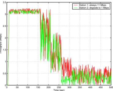
Fig. 1 shows the throughput for two stations, which is run by using the ns-2 simulator [1]. Station 1 always transmits at 11 Mbps while station 2 moves away from the access point (AP) and degrades its data rate to 1 Mbps eventually. The traffic loads for these two stations are saturated, i.e., the queues of these two stations always have packets ready to transmit. The frame sizes for these two stations are fixed as 1500 bytes. It can be seen from Fig. 1 that the throughput of station 1 degrades below 1 Mbps eventually when station 2 transmits at 1 Mbps (i.e., after 300 second). More theoretical and experimental results for the performance anomaly problem can refer to [9].
In the 802.11 series specifications, IEEE 802.11b and IEEE 802.11g standards are backward compatible with the IEEE 802.11 standard. Mobile stations implementing IEEE 802.11g and/or IEEE 802.11b protocols transmit data with higher data rates than those ones implementing basic IEEE 802.11. The performance anomaly problem also incurs and deteriorates the system performance for the backward compatibility case.
In this paper, our work tries to optimize the aggregate throughput for those stations transmitting at a higher data rate by accommodating the channel occupancy times among the stations transmitting at different data rates. The channel occupancy time of a station can be adjusted by tuning its trans-mitted MAC frame size and its values of backoff parameters. Tuning the MAC frame size of a station can adjust its capture
0 50 100 150 200 250 300 350 400 450 500 0 0.5 1 1.5 2 2.5 3 3.5 Time (sec) Throughput (Mbps) Station 1: always 11 Mbps Station 2: degrade to 1 Mbps
Fig. 1. An example for performance anomaly.
time when it seizes the channel. Similarly, tuning the values of backoff parameters of a station can adjust its channel access probability so that the channel occupancy time of the station can be adjusted. We specify an index ratio, called time fairness index (T F I) ratio to quantify the ratio of channel occupancy time among all stations, which is based on the fairness model described in [10].
We post a throughput efficiency problem as follows: how to maximize the total aggregate throughput subject to that the channel occupancy times among the stations transmitting at different data rates are kept at a time fairness index ratio. In the paper, we present a primal formulation for the optimization problem, which is a nonlinear mixed integer pro-gramming problem. We prove that the optimization problem is intractable, i.e., the feasible set of the problem is not convex. A heuristic solution based on a penalty function with gradient-based approach is proposed to solve the formulated problem. The computational experiments are made to show that the approach can avoid the performance anomaly and raise the total aggregate throughput. Some guidelines for regulating the parameters needed for the approach are also drawn in this paper.
We consider a tunable T F I ratio since it can gain the flexibility for system administrators to control the radio re-sources. The anomaly problem aries because of the channel occupancy time of those stations transmitting at a lower data rate is longer than those ones transmitting at a higher data rate. It is easy to conquer the problem by forcing all multi-rate stations to remain the same time occupancy time, i.e., T F I ratio is adjusted to be the fairest case (the ratio is one in the proposed fairness model, which will be described in the following section). However, system administrators might want to have some degree of differentiation among those stations transmitting at different data rates, which can be achieved by adjusting T F I ratio. Therefore, for the sake of flexibility, we would allow T F I ratio to be tunable for system
administrators.
The proposed optimization model could be implemented in the AP, for which it can dynamically control the resource access usages in its single-hop coverage. The algorithm for the optimization model is executed whenever a station initiates to transmit, a station leaves its transmission, or a station changes its data rate in the coverage of the AP. The computed results are then distributed to each station in its coverage via a Beacon message in the next Beacon interval. The AP should maintain a data structure to record the statuses of those stations in its coverage. It is easy to know the entrance and departure of a station by using the (re)association service and disassociation service specified in IEEE 802.11. Each station that intends to transmit data via the AP should first associate with the AP. Moreover, whenever a station leaves, it notifies the AP of its departure. The modulation type used for each station to transmit data is also recorded in the data structure of the AP, which can be obtained by checking the SIGNAL field of the physical layer header transmitted by each station.
The rest of this paper is organized as follows. In Section II, we propose an optimization model, which considers both channel occupancy time and total aggregate throughput. We also prove that the model is intractable, i.e., non-convexity property. Section III presents a penalty function with gradient-based approach to solve the optimization model. In Section IV, we show the effectiveness of the approach via computational experiments and provide some guidelines to regulate the pa-rameters needed for the proposed approach. Some remarkable discussions and conclusion are drawn in Section V.
II. THROUGHPUTEFFICIENCYPROBLEM
In this section, we first introduce the notations and assump-tion that we use to formulate the throughput efficiency prob-lem. Second, a mathematical representation for the problem is presented. Finally, we show the hardness of the formulated problem.
A. Notations and Assumption
The system environment we consider is a single wireless cell coordinated with an AP. Each station that intends to transmit a packet has to forward its packet to the AP, even if the packet is destined for a station located in the same cell. The communication channel is assumed to be error-free and of no obstacle. Besides, there is no hidden terminal problem.
Without loss of generality, we assume that there are r modu-lation types with distinct bit rates in the system, where r ≥ 1. That is, there is a set of data rates R = {R1, R2, · · · , Rr}
that can be used by a station. Stations transmitting at different data rates are categorized into multiple traffic classes. We use nk to denote the number of station transmitting at Rk,
where 1 ≤ k ≤ r. We refer to a packet transmitted at Rk as a class-k packet and a station transmitting at Rk
as a class-k station. Suppose that each class-k packet is of length Lk. The backoff parameter, minimum contention
window size, used for class-k stations are denoted by Wk.
that it has greater differentiation effect than other backoff parameters (e.g., maximum contention window size) [13]. Although other backoff parameters can be also jointly tuned in the optimization model, it will increase the complexity of the problem. Hence, in the optimization model, we choose the parameter that has greatest influence on channel access probability.
Let ρk be the aggregate throughput of all class-k stations,
where 1 ≤ k ≤ r. We estimate ρk based on a renewal reward
process [14] and the estimation is shown in the Appendix. In order to quantify channel occupancy time, we specify a time fairness index (T F I) ratio, which is defined as follows.
T F I = ( Pr k=1nkfk)2 Pr k=1nk( Pr k=1nkfk2)
where fkis the time occupied for a class-k station (1 ≤ k ≤ r)
in the long run, which will be also presented in the Appendix. Given n1, n2, · · · , and nr, T F I converges to 1 when the
the time occupancy time of each station approaches equality, while T F I converges to 1/nk when the channel is equally
shared by all class-k stations.
The fairness index carries four characteristics, which is listing as follows.
1) Population size independence: The index is applicable to any number of users (i.e., stations), finite or infinite. 2) Scale independence: The index is independent of scale,
i.e., the unit of measurement is not matter.
3) Bound: The index is bounded between 0 and 1, where a totally fair system has a fairness of 1 and a totally unfair system has a fairness of 0. That is, fairness can be expressed as a percentage. For example, a system with a fairness of 0.1 could be shown to be fair to 10% of the stations in the system and unfair to 90% of the stations in the system.
4) Continuity: The index is continuous. Any slight change in allocation is shown up in the fairness index.
The fairness index has intuitive interpretation and attractive properties. More illustrative examples are presented in [10] to explain the characteristics of the fairness index.
B. Problem Formulation
The performance anomaly problem aries because that the channel occupancy time of those stations transmitting at a lower data rate is greater than the one of those stations transmitting at a higher data rate. Hence, we try to adjust the channel occupancy time and to maximize the total aggregate throughput at the same time. Suppose that the tunable range for Lk (Wk) is {Lmin, Lmax} ({Wmin, Wmax}), where 1 ≤ k ≤ r. The primal formulation for the problem is as follows. P: max r X k=1 ρk subject to T F I = a a ∈ [0, 1] Lmin≤ Lk ≤ Lmax k = 1, 2, · · · , r Wmin≤ Wk≤ Wmax k = 1, 2, · · · , r
Wk and Lk are integers k = 1, 2, · · · , r
As seen from problem P, it is a nonlinear mixed integer programming problem. In order to solve the problem P, we should realize the hardness of the problem. In nonlinear programming, the watershed between easily solvable problems and intractable ones is not linearity, but convexity [6]. In the following section, we show that problem P is intractable, i.e., it is not an easily solved problem.
C. The Hardness of the Formulated Problem
For convenience, we first relax the integer constraint of problem P and discuss the difficulty of the relaxed problem, P0. P0: max r X k=1 ρk subject to T F I = a a ∈ [0, 1] Lmin≤ Lk≤ Lmax k = 1, 2, · · · , r Wmin≤ Wk≤ Wmax k = 1, 2, · · · , r
The objective function maxPrk=1ρk and the constraint
T F I = a contribute the difficulties of problem P0, which
are nonlinear. We show that the feasible set of problem P0 is not a convex set. This implies that problem P0 is intractable and hence problem P is also intractable.
Theorem 1: Problem P0 is intractable.
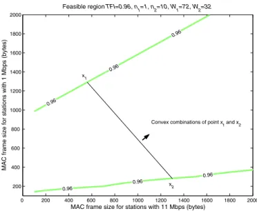
Proof: In order to show the non-convexity property of problem P0, one way we could do is to prove that the feasible set of problem P0 is not a convex set. A set is said to be convex if the line segment joining any two points of the set also belongs to the set. A special case is presented to show the non-convexity property of problem P0. Assume that there are two modulation types supported in the system, i.e., there are two data rates: R1=11 Mbps and R2=1 Mbps. The number of class-1 stations and the number of class-2 stations are one and ten, i.e., n1=1 and n2=10. The minimum contention windows for class-1 stations and class-2 stations are fixed as 72 and 32. T F I is set to 0.96.
We tune the MAC frame sizes for these two classes and show the feasible set of the problem P0, as depicted in Fig. 2. It can be observed form Fig. 2 that the feasible set has two separate regions. We choose two feasible points, which are x1 and x2 indicated in Fig. 2. By expecting x1 and x2, the line segment between x1 and x2 is not feasible. Hence the feasible set of problem P0 is not a convex set. In other words, this implies that the problem P0is not a convex programming problem and is intractable.
Algorithm 1 Sequential Penalty Technique Algorithm Step 1: Initialization.
1) Set iterative time t ← 0
2) Choose initial penalty multiplier µ0 > 0, which is relatively small.
3) Choose a initial feasible solution x(0). 4) Choose an escalation factor β > 1.
Step 2: Linear Constrained Optimization.
Beginning from x(t), solve the problem P” with µ = µt to produce the optimal point x(t+1)
by using the gradient-based algorithm, which is presented Algorithm 2.
Step 3: Stopping.
If x(t+1)is feasible or sufficiently close to feasible in the given constrained problem, i.e., P0, stop and output x(t+1).
Step 4: Advance.
1) Enlarge the penalty multiplier by β, i.e., µt+1= βµt.
2) Set t ← t + 1 and return to Step 2.
Algorithm 2 Gradient-Based Algorithm Step 1: Initialization.
1) Beginning at x(t), choose a feasibility tolerance ² > 0. 2) Set iterative index t ← 0.
Step 2: Step Size.
Choose a number λt as the step size, which is
sufficiently large.
Step 3: Gradient.
Calculate the gradient for the objective function of problem P”, i.e. ∇f (x(t)) = · ∂f (x) ∂x1 ∂f (x) ∂x2 · · · ∂f (x) ∂x2r ¸ . Step 4: Direct.
Assign the moving direction with gradient value, i.e., 4x(t)← ∇f (x(t)).
Step 5: Stationary Point.
If max 1≤i≤2r ½ λt ∂f (x) ∂xi ¾ < ², then x(t) is sufficient to close the stationary point and the algorithm stops. Otherwise, go to the next step.
Step 6: New Point.
1) x(t+1)← x(t)+ λ
t4x(t).
2) If f (x(t+1)< f (x(t))), λ
t= λt/2 and return to Step 3.
Step 7: Advance.
Set t ← t + 1 and return to Step 2.
0 200 400 600 800 1000 1200 1400 1600 1800 2000 200 400 600 800 1000 1200 1400 1600 1800 2000
MAC frame size for stations with 11 Mbps (bytes)
MAC frame size for stations with 1 Mbps (bytes)
Feasible region TFI=0.96, n
1=1, n2=10, W1=72, W2=32 0.96 0.96 0.96 0.96 0.96 0.96
Convex combinations of point x
1 and x2
x 1
x 2
Fig. 2. Non-convexity property of problem P0.
III. PENALTYFUNCTION WITHGRADIENT-BASED
APPROACH
In this section, we first solve problem P0by using a penalty function with gradient-based approach [6]. Then the fractional solution is rounding to integer solution. Considering problem P0, we add a penalty function in the objective function, which
is of the form: P”: max r X k=1 ρk− µ(a − T F I)2 subject to Lmin≤ Lk≤ Lmax k = 1, 2, · · · , r Wmin≤ Wk≤ Wmax k = 1, 2, · · · , r
where µ is the penalty multiplier. The problem P” can be solved by using an iterative algorithm, as shown in Algorithm 1. The penalty multiplier is iteratively increasing to obtain the feasible solution as possible as it can. In each iteration, penalty multiplier is given and the optimum solution of P” is solved by a gradient-based method, as shown in Algorithm 2.
The principle of the penalty approach is to slowly in-crease the penalty multiplier µ to form the sequential penalty technique algorithm. As shown in Algorithm 1, the penalty multiplier µ starts with a relatively small value and grows with each search. For each value of µ, linear constrained penalty problem, i.e., P”, is solved by the gradient-based algorithm, in which the searching begins at the optimum point obtained from the preceding search. If the result is feasible and close to the original problem P0, i.e., T F I is close to a, we stop and obtain a suboptimal solution of problem P0. Otherwise, we continue until the suboptimal solution is sufficiently close to be feasible. The escalation factor β is used to increase the penalty multiplier in the next iteration.
TABLE I
THE VALUES OF PARAMETERS USED IN THE SIMULATION
PHY header 24 bytes
MAC header 40 bytes
ACK 14 bytes Propagation delay 1 µs SIFS 10 µs Slot time 20 µs Lmin 41 bytes Lmax 2304 bytes Wmin 32 Wmax 1024
The sequential increasing technique is necessary for search-ing a good suboptimal point. Why not just use a very large penalty multiplier µ for the first search? When µ is relatively large, the corresponding objective function becomes very steep. That is, a small move from the initial feasible point will result in a dramatic impact on the objective value. Hence, the initial feasible point is hard to move and cannot obtain a good suboptimal point generally. In the gradient-based algorithm, we perform an iterative line search to produce the optimum point after a step size, i.e., λt, is chosen.
The suboptimal point obtained from the approach should be rounding to integer. The rounding method is to choose the best one by comparing 22rpossibilities of combinations. In the next section, we will describe why the basic rounding method can obtain a good suboptimal point in general, which is achieved by some degree of monotonicity property possessed by problem P.
IV. COMPUTATIONALEXPERIMENTS
In the experiment, the physical layer we adopt is the IEEE 802.11b standard [4]. There are four modulation types specified in IEEE 802.11b, under which four data rates (i.e., 11 Mbps, 5.5 Mbps, 2 Mbps and 1 Mbps) are available for data transmission. We only adopt the two-way handshaking mechanism (i.e., DATA-ACK) for all stations to transmit data. The related parameters used in the experiment are summarized in Table I. There are four stations in the system, where their data rates are associated with 1 Mbps, 2 Mbps, 5.5 Mbps and 11 Mbps, respectively, i.e., (n1 n2 n3 n4) = (1 1 1 1) and (R1 R2 R3 R4) = (1 2 5.5 11). In the following subsections, we show the effects of the parameters (i.e., β, µ0 and initial feasible point x(0)) used in the proposed approach, especially in convergence speed and optimality property.
A. Effect of Escalation Factor β
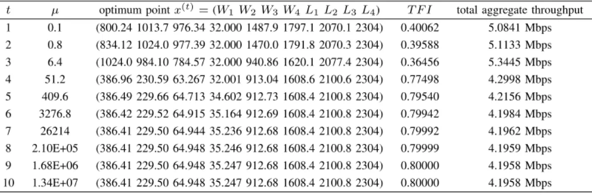
We first demonstrate the convergence speed and optimality property caused by escalation factor β. The value of T F I is set to 0.8. Table II shows the penalty form of sequential penalty technique algorithm (i.e., Algorithm 1) with β = 8. Given the penalty multiplier µ = µ0= 0.1, we start our search from the initial feasible point x(0) = (32 32 32 32 41 41 41 41).
At t = 1, the value of T F I is 0.40062 which violates the first constraint of problem P0 (i.e., T F I = 0.8). Then the multiplier is increased by factor β = 8 and a new search is ini-tiated from the vector x(1). The resulting optimum point, x(1), starts a second search by using µ = µ1 = βµ0. The process continues until µ is large enough so that the suboptimal point approaches feasibility. Hence we stop the procedure and obtain a suboptimal solution x∗ = x(10) = (386.41 229.5 64.948 35.247 912.68 1608.4 2100.8 2304). Table III summarizes the results of sequential penalty technique algorithm with different values of escalation factors β. Observing from Table III, as the value of β is larger, the convergence rate is faster. In addition, the scale of β has not direct impact on the value of suboptimal solution, i.e., total aggregate throughput. However, the initial penalty multiplier µ0 plays an important role and should be considered jointly with escalation factors. In the next section, we show the effect of initial penalty multiplier.
Guideline 1: For the sake of fast convergence speed, the value of escalation factor β should not be assigned with a relatively small value.
B. Effect of Initial Penalty Multiplier µ0
In Table IV, we summarize the results of sequential penalty technique algorithm with different value of initial penalty multiplier µ0, where β = 8, T F I = 0.8, and x(0)= (32 32 32 32 41 41 41 41). It can be seen from Table IV, as the value of initial penalty multiplier is less than 1, the solution can obtain a relatively good suboptimal value. However, the convergence speed is slower as the value of initial penalty multiplier is smaller. When the value of initial penalty multiplier is large enough (e.g., greater than 1000), the convergence speed is fast. However, the suboptimal value of the solution is relatively small.
Guideline 2: The value of initial penalty multiplier is rec-ommendable between 0.1 and 1 to obtain a good suboptimal value with a moderate convergence speed.
C. Effect of Initial Point x(0)
In Table V, we show the performance comparison by starting our search with different initial feasible points. We choose the end points to be our initial feasible points. For eight decision variables (i.e., (x1 x2 x3x4x5x6x7 x8) = (W1W2 W3W4
L1L2L3L4)), we have 28= 256 combinations of end points. Due to the page limit, we select sixteen combinations for illustration. It is remarkable that the practical implementation should compare all the 256 combinations.
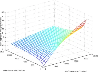
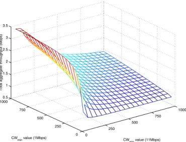
The reason we select end points is that the objective function of problem P0 over its feasible set has some degree of monotonicity property. For convenience of explaining, we show an illustrated example. Assume that there are two classes in the system. Class 1 is for 11 Mbps and class 2 is for 1 Mbps. In Fig. 3, we show the total aggregate throughput versus the MAC frame size, for which the minimum contention window (CWmin) size is (W1 W2) = (32 32) and (n1 n2) = (10 10). In Fig. 4, we show the total aggregate throughput versus the CWmin value, for which the MAC frame size is fixed as (L1
TABLE II
PENALTYFORM WITHβ = 8 (µ0= 0.1, x(0)=(32 32 32 32 41 41 41 41), T F I = 0.8)
t µ optimum point x(t)= (W1W2 W3W4L1L2 L3 L4) T F I total aggregate throughput
1 0.1 (800.24 1013.7 976.34 32.000 1487.9 1797.1 2070.1 2304) 0.40062 5.0841 Mbps 2 0.8 (834.12 1024.0 977.39 32.000 1470.0 1791.8 2070.3 2304) 0.39588 5.1133 Mbps 3 6.4 (1024.0 984.10 784.57 32.000 940.86 1620.1 2077.4 2304) 0.36456 5.3445 Mbps 4 51.2 (386.96 230.59 63.267 32.001 913.04 1608.6 2100.6 2304) 0.77498 4.2998 Mbps 5 409.6 (386.49 229.66 64.713 34.602 912.73 1608.4 2100.8 2304) 0.79540 4.2156 Mbps 6 3276.8 (386.42 229.52 64.915 35.164 912.69 1608.4 2100.8 2304) 0.79942 4.1984 Mbps 7 26214 (386.41 229.50 64.944 35.236 912.68 1608.4 2100.8 2304) 0.79992 4.1962 Mbps 8 2.10E+05 (386.41 229.50 64.948 35.246 912.68 1608.4 2100.8 2304) 0.79999 4.1959 Mbps 9 1.68E+06 (386.41 229.50 64.948 35.247 912.68 1608.4 2100.8 2304) 0.80000 4.1958 Mbps 10 1.34E+07 (386.41 229.50 64.948 35.247 912.68 1608.4 2100.8 2304) 0.80000 4.1958 Mbps TABLE III
SUMMARY OFPENALTYFORMS WITH VARYINGβ (µ0= 0.1, x(0)=(32 32 32 32 41 41 41 41), T F I = 0.8)
β # of iterations suboptimal point x∗= (W1W2W3 W4L1L2L3L4) total aggregate throughput
2 29 (827.75 753.30 146.67 81.293 1244.5 1713.1 2107.5 2304) 3.8843 Mbps 4 15 (719.43 299.95 381.65 72.836 1312.5 1742.2 2090.4 2304) 3.5413 Mbps 8 10 (386.41 229.50 64.948 35.247 912.68 1608.4 2100.8 2304) 4.1958 Mbps 16 9 (656.92 797.86 866.03 137.86 1401.6 1784.0 2095.8 2304) 2.9468 Mbps 32 7 (501.73 153.58 160.39 37.621 1440.7 1784.9 2073.7 2304) 3.8370 Mbps 64 6 (829.42 404.98 795.50 537.94 859.84 1595.7 2085.0 2304) 1.9453 Mbps 128 6 (391.11 801.13 294.39 291.06 1451.9 1788.3 2075.4 2304) 2.1779 Mbps 256 5 (310.09 316.02 86.178 316.38 1386.9 1762.6 2140.8 2304) 2.5377 Mbps 512 5 (627.41 505.15 401.90 79.453 1429.9 1797.0 2132.0 2304) 3.5299 Mbps 1024 4 (853.25 980.49 522.21 125.15 1475.0 1797.1 2077.1 2304) 3.2786 Mbps 2048 4 (393.27 435.58 521.38 284.10 1466.8 1795.9 2077.6 2304) 1.9968 Mbps 4096 4 (408.06 640.59 637.01 156.06 1477.2 1797.3 2075.2 2304) 2.4762 Mbps TABLE IV
SUMMARY OFPENALTYFORMSWITHVARYINGµ0(β = 8, x(0)= (32 32 32 32 41 41 41 41), T F I = 0.8)
µ # of iterations suboptimal point x∗= (W1 W2W3 W4L1L2L3L4) total aggregate throughput
0.0001 15 (718.50 550.53 118.22 67.621 1158.1 1631.3 2051.4 2304.0) 3.9680 Mbps 0.001 13 (381.52 182.59 334.56 50.409 1184.1 1649.8 2043.1 2304.0) 3.5219 Mbps 0.01 12 (408.75 250.18 78.918 254.57 1328.6 1727.6 2140.4 2304.0) 2.7449 Mbps 0.1 11 (386.41 229.50 64.948 35.247 912.68 1608.4 2100.8 2304.0) 4.1958 Mbps 1 10 (628.10 565.93 99.164 55.089 1442.1 1834.1 2055.4 2304.0) 4.0309 Mbps 10 9 (705.39 106.82 99.657 71.826 131.04 283.03 1017.5 1308.2) 2.8179 Mbps 100 7 (317.09 69.380 47.651 35.998 44.710 275.64 528.42 593.81) 1.9756 Mbps 1000 5 (254.61 465.50 130.72 447.81 87.647 349.38 329.52 268.61) 0.8811 Mbps 10000 7 (296.09 63.143 47.495 96.722 41.080 41.236 41.293 41.158) 0.2294 Mbps 100000 4 (407.48 66.856 66.715 110.98 41.040 41.238 41.251 41.155) 0.2218 Mbps 1000000 2 (218.62 292.62 74.464 152.16 41.007 41.005 41.020 41.011) 0.2047 Mbps 10000000 1 (138.98 246.52 49.240 77.419 41.001 41.001 41.000 41.001) 0.2243 Mbps
TABLE V
SUMMARY OFPENALTYFORMSWITHDIFFERENTINITIALFEASIBLEPOINTS(β = 8, µ0= 0.1, T F I = 0.8)
initial feasible point x(0) suboptimal point x∗= (W1 W2W3 W4L1L2L3L4) total aggregate throughput
(32 32 32 32 41 41 41 41) (386.41 229.50 64.948 35.247 912.68 1608.4 2100.8 2304.0) 4.1958 Mbps (32 32 32 32 41 41 2304 2304) (534.87 504.13 444.52 245.05 41.000 41.000 2304.0 2304.0) 3.1960 Mbps (32 32 32 32 2304 2304 41 41) (655.48 368.73 167.17 35.997 2226.4 2303.8 355.02 689.94) 2.0875 Mbps (32 32 32 32 2304 2304 2304 2304) (951.83 844.66 190.15 94.479 1136.1 1834.0 2304.0 2304.0) 3.8452 Mbps (32 32 1024 1024 41 41 41 41) (435.92 266.62 166.72 35.927 1200.5 2304.0 245.63 644.59) 1.9938 Mbps (32 32 1024 1024 41 41 2304 2304) (207.37 118.09 538.92 815.40 41.000 112.38 2304.0 2304.0) 1.5091 Mbps (32 32 1024 1024 2304 2304 41 41) (885.42 516.57 648.88 86.206 2140.1 2304.0 193.80 855.08) 1.8968 Mbps (32 32 1024 1024 2304 2304 2304 2304) (945.49 425.85 102.38 47.844 1916.4 2211.2 2304.0 2304.0) 4.1498 Mbps (1024 1024 32 32 41 41 41 41) (253.42 725.20 319.21 199.14 41.000 63.839 2108.6 2304.0) 3.2569 Mbps (1024 1024 32 32 41 41 2304 2304) (920.28 471.31 553.52 297.78 41.000 41.000 2304.0 2304.0) 3.0208 Mbps (1024 1024 32 32 2304 2304 41 41) (319.13 131.84 32.711 203.80 2070.9 2264.5 1113.7 2304.0) 2.3229 Mbps (1024 1024 32 32 2304 2304 2304 2304) (556.20 537.86 919.39 224.51 41.000 1443.8 2304.0 2304.0) 2.8979 Mbps (1024 1024 1024 1024 41 41 41 41) (506.45 418.32 867.49 113.97 1176.3 1402.0 1536.2 2304.0) 2.9588 Mbps (1024 1024 1024 1024 41 41 2304 2304) (119.42 421.72 201.78 110.67 41.000 41.000 2304.0 2304.0) 3.5431 Mbps (1024 1024 1024 1024 2304 2304 2304 2304) (746.61 779.86 122.12 54.947 2173.9 2273.6 1961.8 2304.0) 3.9595 Mbps (1024 1024 1024 1024 2304 2304 2304 2304) (971.38 868.91 122.04 64.238 2216.1 2284.9 2304.0 2304.0) 3.9922 Mbps
L2) = (2304 2304) and (n1 n2) = (10 10). Both Fig. 3 and Fig. 4 show that the global optima incurs close to one of end points. Therefore, using the end points to be our initial feasible points might have good opportunity to reach the global optima. As seen from Table V, the selection of initial feasible points has great impact on the suboptimal value of the solution. With different initial feasible points, the resulting suboptimal values have great range of differences. It is prefer to try many initial feasible points as possible as we can. However, many comparisons increase the complexity of the algorithm. Hence, we suggest to use end points as initial feasible points and choose the one that produces maximal value.
Guideline 3: The selection of initial feasible point is sug-gested to use end points since the objective function over the feasible set has some degree of monotonicity property. Run all the combinations starting with end points and choose the one that produces maximal value.
D. Effect of Number of Stations
In this section, we show the impact on optimality prop-erty with different numbers of stations. We show that when the number of stations is changing, the sequential penalty technique algorithm should be recalculated to ensure that the suboptimal solution is the best.
We run three scenarios where the related values of parame-ters are the same with Table V excepting the number of mobile stations. The three scenarios are shown in Table VI. The initial feasible points for scenario 1 and scenario 2 are selected from the point that produces the best suboptimal value, i.e., as seen from the first row of Table V, the point is (32 32 32 32 41 41 41 41).
For scenario 3, we select the initial feasible point that produces the second best suboptimal value, i.e., as seen from the eighth row of Table V, the point is (32 32 1024 1024
0 500 1000 1500 2000 2500 0 500 100 1500 2000 2500 0 0.5 1 1.5 2 2.5 3 3.5 4 4.5
MAC frame size (11Mbps) MAC frame size (1Mbps)
Total aggregate throughput (Mbps)
Fig. 3. Total aggregate throughput vs. (L1L2).
2304 2304 2304 2304). Table VI shows the suboptimal values for these three scenarios. It can be seen form Table VI, the resulting suboptimal value of scenario 2 is less than the one of scenario 3. Hence, when the number of stations is changing, the 256 combinations should be recalculated to ensure to obtain the best initial feasible point since the best initial feasible point for (n1 n2 n3 n4) = (1 1 1 1) is not the best initial feasible point for (n1n2 n3 n4) = (1 1 10 1).
Guideline 4: When the number of station in the system is changing, the sequential penalty technique algorithm should be recalculated to obtain the best suboptimal value.
TABLE VI
SUMMARY OFPENALTYFORMWITHVARYING(n1n2n3n4) (β = 8, x(0)= (32 32 32 32 41 41 41 41), T F I = 0.8)
initial feasible point x(0) (n1 n2 n3 n4) total aggregate throughput (Mbps)
(32 32 32 32 41 41 41 41) (1 1 1 1) 4.1958 (32 32 32 32 41 41 41 41) (1 1 10 1) 3.9876 (32 32 1024 1024 2304 2304 2304 2304) (1 1 10 1) 4.0686 0 250 500 750 1000 0 250 500 750 1000 0.5 1 1.5 2 2.5 3 3.5 CWmin value (11Mbps) CWmin value (1Mbps)
Total aggregate throughput (Mbps)
Fig. 4. Total aggregate throughput vs. (W1 W2).
E. Effect of Rounding
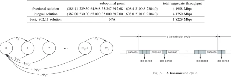
The penalty function with gradient-based approach solves the problem P0and obtains a fractional solution. The fractional solution is then rounding to obtain an integral solution that can produce the maximal value by comparing 22r possible combinations. In Table VII, we show the case by rounding the obtained solution. The integral solution produces worse value than the one of fractional solution. Actually, the val-ues among the 256 integral solutions have little difference. This achievement is caused by the monotonicity property as mentioned before. Therefore, for alleviating the computational efforts of the algorithm, it is suggested to choose any one of integral solutions.
As shown in Table VII, the total aggregate throughput produced by the proposed optimization model is 4.175 Mbps, which is much larger than the one produced by the original IEEE 802.11 protocol, i.e., 1.8229 Mbps.
Guideline 5: Among all the possible integral solutions, they have little difference in the suboptimal value since the objective function over the feasible set has some degree of monotonicity property. In order to save computational time, it is suggested to select any one of integral solutions.
V. CONCLUSION
In this paper, we addressed the performance anomaly prob-lem which is arising when multi-rate traffic is available in
IEEE 802.11 WLANs. Mobile stations transmitting at different data rates are categorized into multiple traffic classes. In order to avoid the performance anomaly problem, we character-ized the channel occupancy times among multiple classes by using a fairness index ratio. With this characterization, we regulate the channel occupancy time by adjusting the minimum contention window sizes and MAC frame sizes among multiple traffic classes. A nonlinear mixed integer programming problem was formulated to maximize the total aggregate throughput. The solution approach was based on a penalty function with gradient-based algorithm. We showed the convergence speed analysis and optimality property anal-ysis. Some examples were also demonstrated to illustrate the effects of selected parameters for the approach.
There are two further research topics. On the one hand, in addition to T F I criterion, the throughput fairness index or delay fairness index criteria could be derived. The criteria can be used to bind to the constraint range for which more realistic solution can be obtained. On the other hand, the proposed capacity estimation model can be used as information for system administrators to manage the radio access resources. The resource management problem, i.e., admission control and bandwidth reservation, in WLAN is a novel topic in future high-speed WLAN. A proper resource management mechanism is desired to ensure that the wireless resources could be effectively utilized.
APPENDIX
AGGREGATETHROUGHPUTANALYSIS
In the appendix, we present the estimation for the aggregate throughput of class-k stations. We first derive the collision probability and transmission probability of a class-k station. With these two probabilities, the aggregate throughput for class-k stations is then analyzed based on a renewal reward process [14]. The analytical model for estimating the aggregate throughput was inspired from [7], [8], [11], [12]. Finally, we present the derivation of fk.
A. Collision Probability and Transmission Probability A discrete and integral time scale is adopted: [t, t + 1) represents a logical time unit, where t ≥ 0 is an integer. Each mobile station decreases its backoff counter or transmits a packet at the beginning of a logical time unit. The length of each logical time unit can be any of the following: the length (i.e., δ) of a time slot, the time length required for a successful transmission, and the time length required for a colliding transmission.
TABLE VII
ROUNDING(µ0= 0.1, β = 8, x(0)=(32 32 32 32 41 41 41 41), T F I = 0.8)
suboptimal point total aggregate throughput
fractional solution (386.41 229.50 64.948 35.247 912.68 1608.4 2100.8 2304.0) 4.1958 Mbps
integral solution (387.00 230.00 65.000 35.000 912.00 1608.0 2101.0 2304.0) 4.1750 Mbps
bacic 802.11 solution N/A 1.8229 Mbps
0 m k m k-1 1
...
pk 1-pk pk 1-pk 1-pk 2 pk 1-p kFig. 5. State transition diagram of Sk(t).
Let pk(t) be the probability of collision when a class-k
station transmits a packet at time t, where 1 ≤ k ≤ r. Like [7], it is assumed that pk(t) = pk for all integers t ≥ 0, i.e., pk(t)
is independent of time. Suppose that the maximum contention window for class-k stations is CWmax = 2mkWk, where mk
is called the maximum backoff stage. Also let Sk(t) be the
backoff stage of a class-k station at time t, where 0 ≤ Sk(t) ≤
mk. Since Sk(t + 1) depends only on Sk(t), {Sk(t) : t ≥ 0}
is a discrete-time Markov chain and the transition diagram is depicted in Fig. 5. By Sk we denote the backoff stage of a
class-k station in steady state. The probability distribution of Sk is given as follows. Pr{Sk= s} = (1 − pk)psk if 0 ≤ s ≤ mk− 1; P∞ j=mk(1 − pk)pjk if s = mk; 0 if s > mk.
Each backoff counter that is generated for a class-k station is randomly determined from [0, 2sWk− 1] in backoff stage
s. Let Bk be a backoff counter for a class-k station, where
0 ≤ Bk ≤ 2mkWk− 1. According to IEEE 802.11 [2], the
probability distribution of Bk in backoff stage s is uniform
[2], i.e., Pr{Bk= i|Sk= s} = 1 2sW k, for 0 ≤ i ≤ 2 sW k− 1.
Consequently, the expected backoff counter for a class-k station in backoff stage s can be computed as follows.
E[Bk|Sk = s] =
2sW k− 1
2 .
Further, the expected backoff counter for a class-k station
collision ... success a transmission cycle
idle period idle period idle period idle period
... success collision ...
Fig. 6. A transmission cycle.
can be easily computed as follows. E[Bk] = mk X s=0 E[Bk|Sk = s]Pr{Sk= s} = Wk− 1 + pkWk Pmk−1 i=0 (2pk)i 2 = (1 − 2pk)(Wk− 1) + pkWk(1 − (2pk) mk) 2(1 − 2pk) ,
where the last equality holds as pk 6= 1/2. If pk = 1/2, E[Bk]
is simply given by omitting the last equality.
Let qk be the probability of a class-k station to transmit a
packet at any given time, which can be computed as follows.
qk = 1
E[Bk] + 1
= 2(1 − 2pk)
(1 − 2pk)(Wk+ 1) + pkWk(1 − (2pk)mk).
With qk, the value of pk can be computed as follows.
pk= 1 − (1 − qk) Y 1≤j≤r j6=k (1 − qj)nj .
Solving the 2r simultaneous equations for pk and qk by
numerical techniques, e.g., Newton-Raphson method, we can obtain the values of pk and qk.
B. Aggregate Throughput
When multiple stations contend the channel at the same time, there may be several idle periods and colliding trans-missions before a successful transmission. The time interval between two consecutive successful transmissions is referred to as a transmission cycle. Refer to Fig. 6, where each idle period is caused due to the backoff procedure. A new transmission cycle is initiated immediately after a successful transmission.
p = Pr{# of active nodes ≥ 2 | # of active nodes ≥ 1}
= 1 − Pr{# of active nodes = 0} − Pr{# of active nodes = 1} Pr{# of active nodes ≥ 1} = 1 − Q 1≤j≤r(1 − qj)nj− Pr i=1niqi(1 − qi)ni−1 Q 1≤j≤r j6=i (1 − qj) nj 1 −Q1≤j≤r(1 − qj)nj .
Now, the aggregate throughput for class-k stations is ana-lyzed based on a renewal reward process. Here the aggregate throughput means the average bandwidth. Suppose that a station will win a reward if it makes a successful transmission. We define the reward to be the number of bits successfully transmitted. According to renewal arguments [14], in steady state, the reward earned by class-k stations per unit time, i.e., the average bandwidth for all class-k stations, is equal to the expected reward earned by a class-k station during a transmission cycle divided by the expected time length of a transmission cycle.
By Rk(t) we denote a renewal reward process that
repre-sents the reward earned by class-k stations from time zero to time t. The average bandwidth for class-k stations is given as follows. ρk = lim t→∞ Rk(t) t = Fk TS+ TC+ TI,
where Fkis the expected number of bits successfully
transmit-ted for a class-k station and TI (TC and TS, respectively) is
the average time length of idle periods (colliding transmission periods and the successful transmission period, respectively), all during a transmission cycle. The computations of Fk, TS,
TC and TI are detailed in the rest of this section.
Suppose that each class-k packet has length of Lk. Then,
Fk = gkLk, where gk is the probability that a class-k packet
is successfully transmitted during a transmission cycle. The value of gk can be computed as follows.
gk = Pr{active node is class-k|# of active nodes = 1}
= nkqk(1 − qk)nk−1 Q 1≤j≤r j6=k (1 − qj) nj Pr i=1niqi(1 − qi)ni−1 Q 1≤j≤r j6=i (1 − qj) nj.
Let TP HY, TM AC, TACK, TRT S, and TCT S be the time
lengths required to transmit a physical layer header, a MAC layer header, an ACK, an RTS, and a CTS respectively. Also, by TDIF S we denote the time length required for a DCF
interframe space (DIFS). Assume that the propagation delay for all packets is π. According to IEEE 802.11 [2], we have TS = TDIF S+TP HY+TM AC+
Pr
k=1Fk/Rk+π +TP HY+
TM AC + TACK+ π if the two-way handshaking is adopted,
and TS = TDIF S+ TP HY + TM AC+ TRT S+ TSIF S+ π +
TP HY + TM AC+ TCT S+ TSIF S+ π + TP HY + TM AC +
+TSIF S+
Pr
k=1Fk/Rk+ π + TP HY + TM AC+ TACK+ π
if the four-way handshaking is adopted.
Let C be the number of colliding transmissions in a transmission cycle. Then, TC is equal to E[C] multiplied
by the time length of each colliding transmission period. The latter can be computed as TDIF S+ TP HY + TM AC +
Pr
k=1Fk/Rk+ π if the two-way handshaking is adopted, and
TDIF S+ TP HY + TRT S+ π if the four-way handshaking is
adopted.
The probability distribution of C is given as follows. Pr{C = i} = (1 − p)pi, for i ≥ 0,
where p is the probability of collision when a station transmits a packet. It is easy to obtain E[C] = 1−pp . The computation of p is shown at the top of this current page.
Assume that the time lengths of idle periods are indepen-dently and identically distributed. Let I be the number of time slots contained in an idle period. Then, TI = (E[C] + 1) ×
δ × E[I] (refer to Fig. 6). The probability distribution of I is given as follows. Pr{I = i} = 1 − Y 1≤j≤r (1 − qj)nj × Y 1≤j≤r (1 − qj)nj i , for i ≥ 0. It is easy to obtain E[I] = ∞ X i=0 i 1 − Y 1≤j≤r (1 − qj)nj Y 1≤j≤r (1 − qj)nj i = Q 1≤j≤r(1 − qj)nj 1 −Q1≤j≤r(1 − qj)nj .
C. Channel Occupancy Time for a Class-k Station - fk
Observing from Fig. 6 again, the long-term channel oc-cupancy time for a class-k station can also consider the transmission behavior during a transmission cycle. Let TS,k
be the time length required for class-k stations to make a successful transmission during a transmission cycle. It is easy to compute that TS,k= TDIF S+ TP HY + TM AC+ Lk/Rk+
π + TP HY+ TM AC+ TACK+ π if the two-way handshaking
is adopted, and TS,k = TDIF S+ TP HY + TM AC+ TRT S+
TSIF S+ π + TP HY+ TM AC+ TCT S+ TSIF S+ π + TP HY+
TM AC+ TSIF S+ Lk/Rk+ π + TP HY + TM AC+ TACK+ π
if the four-way handshaking is adopted. In order to reflect the control overhead caused by backoff behavior and/or collision, we distribute the control overhead according to their ability to
capture the channel (recall the definition of gk). Therefore, fk
can be expressed as follows.
fk =gk(TC+ TI + TS,k)
nk(TC+ TI+ TS).
REFERENCES
[1] The network simulator ns-2, [online] available at
http://www.isi.edu/nsnam/ns/
[2] Wireless LAN Medium Access Control (MAC) and Physical Layer (PHY)
Specifications, IEEE Standard 802.11, 1999.
[3] Wireless LAN Medium Access Control (MAC) and Physical Layer (PHY)
Specifications: High-speed Physical Layer in the 5 GHZ Band, IEEE
Standard 802.11a, 1999.
[4] Wireless LAN Medium Access Control (MAC) and Physical Layer (PHY)
Specifications: High-speed Physical Layer Extension in the 2.4GHz Band, IEEE Standard 802.11b, 1999.
[5] Wireless LAN Medium Access Control (MAC) and Physical Layer (PHY)
Specifications: Further Higher-speed Physical Layer Extension in the 2.4GHz Band, IEEE Standard 802.11g/D3.0, 2002.
[6] M. S. Bazaraa, H. D. Sherali, and C. M. Shetty, Nonlinear Programming, John Wiley & Sons, second edition, 1993.
[7] G. Bianchi, ”Performance analysis of the IEEE 802.11 distributed coor-dination function,” IEEE Journal of Selected Areas in Communications, vol. 18, pp. 535-547, March 2000.
[8] F. Cali, M. Conti, and E. Gregori, ”Dynamic tuning of the IEEE 802.11 protocol to achieve a theoretical throughput limit,” IEEE/ACM
Transactions on Networking, vol. 8, pp. 785-799, December 2000.
[9] M. Heusse, F. Rousseau, G. Berger-Sabbatel, and A. Duda, ”Perfor-mance anomaly of 802.11b”, Proceedings of the IEEE International
Conference on Computer Communication (INFOCOM), April 2003, pp.
836-843.
[10] R. Jain, D. Chiu, and W. Hawe, ”A quantitative measure of fairness and discrimination for resource allocation in shared computer systems,”
DEC, Research Repeport TR-301, 1984.
[11] Y. L. Kuo, C. H. Lu, E. H. K. Wu, and G. H. Chen, ”Performance analysis of enhanced distributed coordination function in IEEE 802.11e,”
Proceedings of the IEEE Vehicular Technology Conference (VTC) Fall,
vol. 3, Orlando U.S., pp. 1412-1416, October 2003.
[12] Y. L. Kuo, C. H. Lu, E H. K. Wu, and G. H. Chen, ”An admission control strategy for differentiated services in IEEE 802.11,” Proceedings of the
IEEE Global Communications Conference (GLOBECOM), vol. 2, San
Francisco, December 2003, pp. 707-712.
[13] Y. L. Kuo, E. H. K. Wu, and G. H. Chen, ”MAC protocol enhancement for QoS provisioning in the IEEE 802.11 wireless LANs: a perfor-mance analysis,” NTU Technical Report, 2003, [online] available at http://inrg.csie.ntu.edu.tw/˜laner/analytical model.pdf
[14] S. M. Ross, Introduction to Probability Models, Academic Press, eighth edition, 2003.