近似無關分量迴歸

科技部補助專題研究計畫成果報告

期末報告

近似無關分量迴歸

計 畫 類 別 ： 個別型計畫

計 畫 編 號 ： MOST

103-2410-H-004-014-執 行 期 間 ： 103年08月01日至104年07月31日

執 行 單 位 ： 國立政治大學經濟學系

計 畫 主 持 人 ： 林馨怡

計畫參與人員： 碩士級-專任助理人員：羅杏芳

碩士班研究生-兼任助理人員：李崇凱

處 理 方 式 ：

1.公開資訊：本計畫可公開查詢

2.「本研究」是否已有嚴重損及公共利益之發現：否

3.「本報告」是否建議提供政府單位施政參考：否

中　華　民　國　104　年　10　月　22　日

中 文 摘 要 ： 考量外匯市場的通貨彼此有同期相關，本研究計劃使用分量迴歸方

法，結合近似不相關迴歸模型，用以分析遠期匯率不偏性假說。本

研究計劃有二大貢獻，第一，提出一個結合分量迴歸及近似不相關

迴歸模型的新估計方式，且由本計劃的蒙地卡羅模擬可知，本計劃

所提的方法的小樣本表現良好，因此未來將可應用到多種議題。第

二，本計劃的國際金融實證發現遠期匯率是即期匯率的偏誤估計式

，而且此偏誤會隨著即期匯率的變化程度而有不同，故支持

Huisman et al (1998)的分析。

中 文 關 鍵 詞 ： 遠期匯率，即期匯率，分量迴歸，近似不相關迴歸模型

英 文 摘 要 ：

英 文 關 鍵 詞 ：

1

Introduction

Is the forward exchange rate a good predictor of the future spot exchange rate?

When the foreign exchange market is efficient, following the argument of Fama

(1970), the forward exchange rate should be an unbiased predictor of the future

spot exchange rate. The resulting theory is the “forward rate unbiasedness

hy-pothesis” from Levich (1979). The hypothesis is an important issue in the field of

international finance. Many researchers are devoted to test this hypothesis. For

example, the studies of Cornell (1977), Levich (1979) and Frankel (1980) support

the hypothesis. More recent contributions to the linterature include Cornell (1989),

Bilson (1981), Fama (1984), Froot and Frankel (1989), Lewis (1989), Froot (1990),

Engel (1996) and Campbell et al. (2007), among others. They find the forward

exchange rate to be a biased predictor of the future spot exchange rate. In

addi-tion, since the foreign exchange markets are subject to common external shocks, a

contemporaneous correlation between currencies is inevitable. Thus, the seemingly

unrelated regression (SUR) model is used to test the validity of the forward rate

un-biasedness hypothesis (Bailey et al, 1984; Chiang, 1988; Doroodian and Albarano,

1998; Frankel and Poonawala, 2010).

Moreover, it is noted that the bias of forward exchange rate depends on the

amount of the future change in the spot exchange rate.

Huisman et al (1998)

find that the bias is small in large change of spot exchange rate and is large in

small change of spot exchange rate. Lobo and Tufe (1998) argue that the exchange

rates are dynamic correlated and are asymmetry. Rogoff (1977), Hansen and Hodric

(1980) and Frankel (1980) point out that exchange rates are non-normal distribution.

According to these characteristics, the quantile regression method, instead of the

ordinary least square technique, should be considered when testing the forward rate

unbiasedness hypothesis. Therefore, a feasible method of quantile regression for the

SUR model is needed. To the best of our knowledge, Jun and Pinkse (2009) is the

only theoretical research on quantile regression for SUR model. Jun and Pinkse

(2009), following Zhao’s (2001) weighted quantile regression, propose an efficient

semiparametric estimator of a multivariate linear regression model. They show that

the proposed estimator is asymptotical and they obtain good simulation results.

However, since Jun and Pinkse (2009) use the nonparametric estimating method, it

is difficult to apply their method for large number of equations. For example, Jun

and Pinkse (2009) do not even provide simulation results in their paper for number

of equation larger than 3. In the empirical research of forward rate unbiasedness

hypothesis, the number of currencies used are large, which makes the method of Jun

and Pinkse (2009) not feasible. Therefore, one motivation of this paper is to propose

an alternative on quantile regression for SUR model and apply the proposed method

to test the forward rate unbiasedness hypothesis.

In this paper, we propose a quantile regression method for SUR model. The

Monte Carlo simulation is provided to show that the proposed method has better

small sample performances. We then apply the proposed method to investigate the

forward rate unbiasedness hypothesis. Our empirical results show that the forward

exchange rate is biased and the bias depends on the amount of the future change in

the spot exchange rate. When the amount of the future change in the spot exchange

is large, the biased is small and vice versa. Our empirical results are consistent with

those in Huisman et al (1998).

The remainder of this paper is organized as follows. Section 2 provides the

literature review. The econometric methodology are presented in Section 3. In

Section 4, I discuss the empirical study of the paper. Section 5 concludes the paper.

2

Literature review

Forward rate unbiasedness hypothesis, proposed by Levich (1979), is one of the

fun-damental theoretical building blocks for understanding the behavior of spot exchange

rate in foreign exchange markets. Forward rate unbiasedness hypothesis implies that

the forward exchange rate is an unbiased predictor of the future spot exchange rate.

Cornell (1977), Levich (1979), and Frankel (1980) regress spot exchange rate on

forward exchange rate and their results support the hypothesis. However, the

em-pirical studies of Bilson (1981), Fama (1984), and Froot and Frankel (1989) reject

the hypothesis. Various researches have been proposed for this rejection, such as

Froot and Frankel (1989), Lewis (1989, 1995), Engel (1996) and Campbell et al.

(2007). Froot and Frankel (1989), Lewis (1989), and Campbell et al. (2007) argue

that the foreign exchange market is not efficient because invests do not have rational

expectations. Most traders are risk aversion within the market, and there exists risk

premium, e.g. Fama (1984), Engel (1996b).

Since the foreign exchange markets are subject to common external shocks, the

SUR model is used to test the validity of the forward rate unbiasedness hypothesis.

Bailey et al. (1984) use weekly data of spot and 3–day forward exchange rates of

the UK pound, Germany mark, Italian lira, and French franc to test the hypothesis

and their results reject the hypothesis. Chiang (1988) uses monthly data of spot

and 30-day forward exchange rates of the Canadian dollar, French franc, Germany

mark and UK pound to test the hypothesis and the results support the hypothesis.

Doroodian and Albarano (1998) use monthly data of spot and forward exchange

rates of the Canadian dollar, French franc, Germany mark and Swiss Franc, and

show the exchange markets are inefficient.

Most studies of forward rate unbiasedness hypothesis focus on advanced

mar-ket currencies and find that the coefficient of forward exchange rate is biased and

negative. Frankel and Poonawala (2010) first test for bias in the forward markets

in emerging market currencies, and to see how the bias compares to that for major

currencies. Frankel and Poonawala (2010) use monthly data of spot and 1-month

forward exchange rates of 21 advanced country currencies and 14 emerging

coun-try currencies. Their results reject the hypothesis and the bias of advanced market

currencies are larger than that of emerging market currencies.

In the existing literature, the ordinary least square method is used for the SUR

model on the forward rate unbiasedness hypothesis. However, in foreign exchange

markets, it may occur peso problem. In an open environment, the expected impact

of catastrophic events will be further spread and strengthened. People will expect

depreciation in the future because overvalue the currency, making the expected

depreciation to be self-realization. Thus, the change of exchange rates is not normal

distributed. Rogoff (1977), Hansen and Hodric (1980) and Frankel (1980) point out

that exchange rates are non-normal distribution. In addition, Lobo and Tufe (1998)

argue that the exchange rates are dynamic correlated and are asymmetry. Huisman

et al. (1998) find that the bias is small in large change of spot exchange rate and is

large in small change of spot exchange rate. According to these characteristics, the

quantile regression method, instead of the ordinary least square technique, should

be considered when testing the forward rate unbiasedness hypothesis.

3

Seemingly Unrelated Quantile Regression

3.1

Model and estimation

The ordinary SUR model is to stack the data and to estimate parameters by

gener-alized least square estimation. Following this procedure, we stack data to construct

a SUR model and then estimate the model by quantile regression. The resulting

estimation method is called “stacking quantile regression”. For example, consider

two regression equations as follows.

y

= x

0

t

β

+ ε

, Q(ε

|x

) = 0, t = 1, . . . , T,

where Q(·|·) is the conditional quantile function,

y

=

"

y

y

#

,

x

=

"

x

0

0

x

#

,

β

=

"

β

β

#

.

Or equivalently,

y

= x

β

+ ε

, i = 1, 2; t = 1, · · · , T,

where y

∈ R

, x

∈ R

, β

is a vector of parameters, and K is total number of

unknown regression coefficients. This paper suggests using the quantile regression

technique to estimate the stacked data to obtain the parameters of interest.

In this paper, we provide some preliminary simulation results to show that the

proposed method is feasible. In our Monte Carlo simulation, we compare three

estimators: the stacking quantile regression of this paper, the weighted quantile

re-gression of Zhao (2001), and the estimator of Jun and Pinkse (2009). The estimating

procedure of Jun and Pinkse (2009) is in the following:

Step1 Run regression for each equation uses quantile regression:

ˆ

β

= arg min

X

τ |y

− x

β

| +

X

(1 − τ )|y

− x

β

|,

ˆ

β

= arg min

X

τ |y

− x

β

| +

X

(1 − τ )|y

− x

β

|.

Save the residuals ˆ

ε

and ˆ

ε

.

Step2 Suppose that w

are the k-nearest neighbor (KNN) weights, satisfying

T

X

d=1

w

= 1, w

= 0, w

≥ 0, t, d = 1, 2, · · · , T.

The kernel density estimator of ε

at zero is defined as

ˆ

F

=

"

I

/(2θ

)

0

0

I

/(2θ

)

#

,

where ι is a vector of ones, and θ

is a bandwidth parameter. Then, we can

obtain

ˆ

S

=

X

w

F

ˆ

x

.

Step3 Compute

ˆ

G

=

X

w

ˆ

s

s

ˆ

,

with ˆ

s

= I

− τ . Then, we obtain ˆ

A

= ˆ

S

t

G

ˆ

.

Step4 Use linear programming technique to solve the following moment condition:

1

T

X

ˆ

A

(I

− τ ) = 0.

Finally the estimator

β is obtained by Newton step.

ˆ

ˆ

3.2

Monte Carlo Simulation

The data generating process of our experiment follows Jun and Pinkse (2009):

y

= β

+ β

x

+ β

x

+ ε

, i = 1, 2, · · · , N, t = 1, 2, · · · , T,

where T is the sample size, N is the total number of equations, and β

= [β

β

β

]

0

=

[10 − 4 2]

. In addition, the regressors x

, x

and ε

are generated using the

following design:

x

= N

+ 0.2U

, x

= 0.2N

+ U

, ε

= h

(X

)e

,

where N

∼ N (5, 9) , U

∼ U (0, 4). In the homoskedastic experiments we set

h

= 1 and the heteroskedastic form used is

h

(X

) = exp(|x

β

+ x

β

+ x

β

|/10),

h

(X

) = 1 + 3exp(−(x

β

+ x

β

+ x

β

+ 10)

/100),

where x

= [1 x

x

]

0

. The number of replication is 1000. We calculate

bias and root mean squared error (RMSE) for the three estimators. We list all

the simulation results in the Appendix and provide more explanations in the future

version of this paper.

4

Empirical Study

4.1

Data and Empirical Models

The data used in the paper is based on those in Frankel and Poonawala (2010).

There are 10 advanced market currencies, including the Australian dollar, Canadian

dollar, Danish krone, Euro, Japanese yen, New Zealand dollar, Norwegian krone,

Swedish Krona, Swiss franc and UK pound. Also, there are 14 emerging market

cur-rencies, including the Czechoslovakia koruna, Hong Kong dollar, Hungarian forint,

Indian rupee, Indonesia rupiah, Kuwaiti dinar, Mexican peso, Philippine peso, Saudi

Arabian riyal, Singapore dollar, South African rand, Taiwan dollar, Thai baht and

Turkish@lira. The monthly data of spot and 1-month forward exchange rate are

collected over the period of December 31, 1998 to March 29, 2013, and from the

Datastream.

Table 13 and Table 14 present descriptive statistics of our data. To test the

normality of future change of currencies, we use Jarque-Bera test and the results

are shown in Table 15. This table shows that most of the future change in the spot

exchange rate of each currency is right-skewed and heavy-tailed. Therefore, the

quantile regression should be considered to fully describe the distribution of future

change in the spot exchange rate. In addition, the daily data are also considered.

Table 16 and Table 17 present descriptive statistics and Table 18 show the results

of Jarque-Bera test.

Our empirical study is based on the following model:

s

− s

= α + β(f

− s

) + ε

,

where s

is log of the spot exchange rate at time t, f

is log of the forward exchange

rate at time t, s

− s

is the future change in the spot exchange rate, f

− s

is

the forward premium. The null hypothesis of unbiasedness is β = 1. The stacking

quantile regression is applied to test this hypothesis.

4.2

Empirical Results

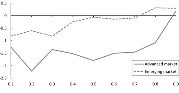
Figure 1 shows the average of ˆ

β(τ ) for advanced and emerging market currencies

under different quantiles. From Figure 1 we can see that the coefficients are smaller

in absolute values in emerging countries than those in advanced market. The results

are consistent with Frankel and Poonawala (2010) where they show a larger bias in

                                                              ‐2.5 ‐2 ‐1.5 ‐1 ‐0.5 0 0.5 0.1 0.2 0.3 0.4 0.5 0.6 0.7 0.8 0.9 Advanced market Emerging market

Figure 1: Spot on forward regression–monthly data

advanced market than in emerging market. In addition, the bias decreases along with

quantiles in absolute value; which shows that the forward exchange rate is biased

and the bias depends on the amount of the future change in the spot exchange rate.

When the amount of the future change in the spot exchange is large, the bias is

small and vice versa. Our empirical results are consistent with those in Huisman et

al (1998). The empirical result of daily data are presented in Figure 2. We have

similar conclusion for daily data.

5

Conclusions

In this paper, we propose a quantile regression method for SUR model. The Monte

Carlo simulation is provided to show that the proposed method has better small

sample performances. The empirical results show that a larger bias in advanced

market than in emerging market, which is consistent with Frankel and Poonawala

(2010). In addition, we also show that, when the amount of the future change in the

spot exchange is large, the bias is small and vice versa. Our results do not support

                                                              ‐0.6 ‐0.5 ‐0.4 ‐0.3 ‐0.2 ‐0.1 0 0.1 0.2 0.1 0.2 0.3 0.4 0.5 0.6 0.7 0.8 0.9 Advanced market Emerging market

Figure 2: Spot on forward regression–daily data

the “forward rate unbiasedness hypothesis” and is consistent with Huisman et al

(1998).

References

Bailey, R. W., Baillie, R. T., McMahon, P. C., 1984. Interpreting econometric

evidence on efficiency in the foreign exchange market. Oxford Economic Papers

36, 67–85.

Bilson, J. F. O., 1981. The speculative efficiency hypothesis. The Journal of

Busi-ness 54, 435–451.

Campbell, R., Kees, K., Lothian, J., Mahieu, R., 2007. Irving Fisher, expectational

errors, and the UIP puzzle. Centre for Economic Policy Research discussion

paper, 6294.

Chiang, T. C., 1988. The forward rate as a predictor of the future spot rate: A

stochastic coefficient approach. Journal of Money, Credit and Banking 20,

212–232.

Cornell, B., 1977. Spot rates, forward rates and exchange market efficiency. Journal

of Financial Economics 5, 55–65.

Cornell, B., 1989. The impact of data errors on measurement of the foreign exchange

risk premium. Journal of International Money and Finance 8, 147–157.

Doroodian, C. J. K., Albarano, R., 1998. The unbiased forward rate hypothesis: A

re-examination. Applied Financial Economics 8, 567–575.

Engel, C., 1996. The forward discount anomaly and the risk premium: a survey of

recent evidence. Journal of Empirical Finance 3, 123–191.

Engel, C., 1996b. A note on cointegration and international capital market efficiency.

Journal of International Money and Finance 15, 657–660.

Fama, E. F., 1970. Efficiency capital markets: A review of theory and empirical

work. Journal of Finance 25, 383–471.

Fama, E. F., 1984. Forward and spot exchange rates. Journal of Monetary

Eco-nomics 14, 319–338.

Frankel, J. A., 1980. Tests of rational expectations in the forward exchange market.

Southern Economic Journal 46, 1083–110.

Frankel, J. A., Poonawala J., 2010. The forward market in emerging currencies: Less

biased than in major currencies. Journal of International Money and Finance

29, 585–598.

Froot, K. A., Frankel, J. A., 1989. Forward discount bias: is it an exchange risk

premium? Quarterly Journal of Economics 104, 139–161.

Froot, K. A., 1990. Short rates and expected asset returns. NBER, Cambridge,

MA, working paper, 3247.

Hansen, L. P., Hodrick, R. J., 1980. Forward exchange rates as optimal predictors

of future spot rates: an econometric analysis. Journal of Political Economy

88, 829–853.

Huisman, R., Koedijk, K., Kool, C., Nissen, F., 1998. Extreme support for

uncov-ered interest parity. Journal of International Money and Finance 17, 211–228.

Jun, J. S., Pinkse, J., 2009. Efficient semiparametric seemingly unrelated quantile

regression estimation. Econometric Theory 25, 1392–1414.

Levich, R. M., 1979. Are forward exchange rates unbiased predictors of future spot

rates? Columbia Journal of World Business 14, 49–61.

Lewis, K. K., 1989. Changing beliefs and systematic rational forecast errors with

evidence from foreign exchange. American Economic Review 79, 621–636.

Lobo, B. J., Tufte, D., 1998. Exchange rate volatility: Does politics matter? Journal

of Microeconomics 20, 351–365.

Rogoff, K., 1977. Rational expectations in the foreign exchange market revisited.

Unpublished paper, MIT.

Zhao, Q., 2001. Asymptotically efficient median regression in the presence of

het-eroskedasticity of unknown form. Econometric Theory 17, 765–784.

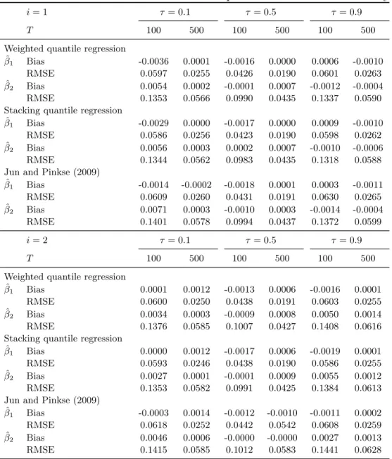
Table 1: Bias and RMSE for different sample size with homoskedasticity

i = 1 τ = 0.1 τ = 0.5 τ = 0.9 T 100 500 100 500 100 500 Weighted quantile regression

ˆ β1 Bias -0.0036 0.0001 -0.0016 0.0000 0.0006 -0.0010 RMSE 0.0597 0.0255 0.0426 0.0190 0.0601 0.0263 ˆ β2 Bias 0.0054 0.0002 -0.0001 0.0007 -0.0012 -0.0004 RMSE 0.1353 0.0566 0.0990 0.0435 0.1337 0.0590 Stacking quantile regression

ˆ β1 Bias -0.0029 0.0000 -0.0017 0.0000 0.0009 -0.0010 RMSE 0.0586 0.0256 0.0423 0.0190 0.0598 0.0262 ˆ β2 Bias 0.0056 0.0003 0.0002 0.0007 -0.0010 -0.0006 RMSE 0.1344 0.0562 0.0983 0.0435 0.1318 0.0588 Jun and Pinkse (2009)

ˆ β1 Bias -0.0014 -0.0002 -0.0018 0.0001 0.0003 -0.0011 RMSE 0.0609 0.0260 0.0431 0.0191 0.0630 0.0265 ˆ β2 Bias 0.0071 0.0003 -0.0010 0.0003 -0.0014 -0.0004 RMSE 0.1401 0.0578 0.0994 0.0437 0.1372 0.0599 i = 2 τ = 0.1 τ = 0.5 τ = 0.9 T 100 500 100 500 100 500 Weighted quantile regression

ˆ β1 Bias 0.0001 0.0012 -0.0013 0.0006 -0.0016 0.0001 RMSE 0.0600 0.0250 0.0438 0.0191 0.0603 0.0255 ˆ β2 Bias 0.0034 0.0003 -0.0009 0.0008 0.0050 0.0014 RMSE 0.1376 0.0585 0.1007 0.0427 0.1408 0.0616 Stacking quantile regression

ˆ β1 Bias 0.0000 0.0012 -0.0017 0.0006 -0.0019 0.0001 RMSE 0.0593 0.0246 0.0438 0.0190 0.0586 0.0255 ˆ β2 Bias 0.0027 0.0001 -0.0001 0.0009 0.0055 0.0012 RMSE 0.1353 0.0582 0.0991 0.0425 0.1384 0.0613 Jun and Pinkse (2009)

ˆ β1 Bias -0.0003 0.0014 -0.0012 -0.0010 -0.0011 0.0002 RMSE 0.0618 0.0252 0.0442 0.0542 0.0608 0.0259 ˆ β2 Bias 0.0046 0.0006 -0.0000 -0.0000 0.0027 0.0013 RMSE 0.1415 0.0585 0.1012 0.0583 0.1441 0.0628 Notes: eit∼ N (0, 1) , ρ = 0 , replication=1000.

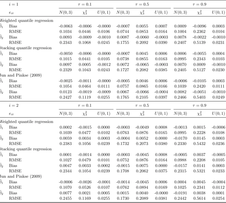
Table 2: Bias and RMSE for different error distribution with homoskedasticity

ˆ β1 Bias -0.0063 -0.0006 -0.0000 -0.0007 0.0055 0.0007 0.0009 -0.0096 0.0003 RMSE 0.1034 0.0446 0.0106 0.0744 0.0853 0.0164 0.1004 0.2362 0.0104 ˆ β2 Bias 0.0093 -0.0009 -0.0010 0.0087 -0.0060 -0.0003 0.0078 -0.0022 -0.0010 RMSE 0.2343 0.1068 0.0245 0.1755 0.2092 0.0390 0.2407 0.5139 0.0231 Stacking quantile regression

ˆ β1 Bias -0.0050 -0.0006 -0.0000 -0.0007 0.0045 0.0006 0.0006 -0.0055 0.0004 RMSE 0.1015 0.0441 0.0105 0.0738 0.0855 0.0163 0.0995 0.2343 0.0103 ˆ β2 Bias 0.0097 0.0005 -0.0012 0.0072 -0.0065 -0.0003 0.0070 0.0009 -0.0010 RMSE 0.2329 0.1043 0.0243 0.1727 0.2082 0.0385 0.2405 0.5127 0.0230 Jun and Pinkse (2009)

ˆ β1 Bias -0.0025 -0.0011 -0.0000 -0.0005 0.0046 0.0006 -0.0006 -0.0105 0.0003 RMSE 0.1054 0.0464 0.0111 0.0757 0.0865 0.0166 0.1039 0.2420 0.0111 ˆ β2 Bias 0.0123 -0.0019 -0.0009 0.0067 -0.0066 -0.0004 0.0082 -0.0051 -0.0010 RMSE 0.2427 0.1119 0.0255 0.1765 0.2105 0.0397 0.2466 0.5403 0.0249 i = 2 τ = 0.1 τ = 0.5 τ = 0.9 eit N (0, 3) χ23 U (0, 1) N (0, 3) χ23 U (0, 1) N (0, 3) χ23 U (0, 1) Weighted quantile regression

ˆ β1 Bias 0.0002 -0.0015 0.0000 -0.0003 -0.0049 0.0008 -0.0013 0.0015 -0.0006 RMSE 0.1039 0.0477 0.0102 0.0763 0.0876 0.0165 0.0995 0.2228 0.0108 ˆ β2 Bias 0.0059 0.0034 0.0003 -0.0004 0.0052 0.0000 -0.0170 0.0145 0.0003 RMSE 0.2383 0.1056 0.0239 0.1732 0.2073 0.0380 0.2330 0.5432 0.0236 Stacking quantile regression

ˆ β1 Bias 0.0001 -0.0014 0.0000 -0.0003 -0.0045 0.0008 -0.0005 0.0037 -0.0005 RMSE 0.1027 0.0479 0.0101 0.0752 0.0876 0.0164 0.0988 0.2208 0.0105 ˆ β2 Bias 0.0047 0.0033 0.0002 -0.0015 0.0075 0.0000 -0.0157 0.0141 0.0003 RMSE 0.2344 0.1054 0.0239 0.1708 0.2062 0.0375 0.2315 0.5321 0.0233 Jun and Pinkse (2009)

ˆ β1 Bias -0.0006 -0.0026 -0.0001 -0.0014 -0.0045 0.0006 0.0004 0.0045 -0.0004 RMSE 0.1070 0.0526 0.0107 0.0762 0.0894 0.0169 0.1025 0.2341 0.0112 ˆ β2 Bias 0.0077 0.0021 0.0005 0.0015 0.0040 -0.0000 -0.0191 0.0038 0.0001 RMSE 0.2455 0.1169 0.0255 0.1730 0.2089 0.0381 0.2442 0.5614 0.0254 Notes: T = 100, ρ = 0 , replication=1000.

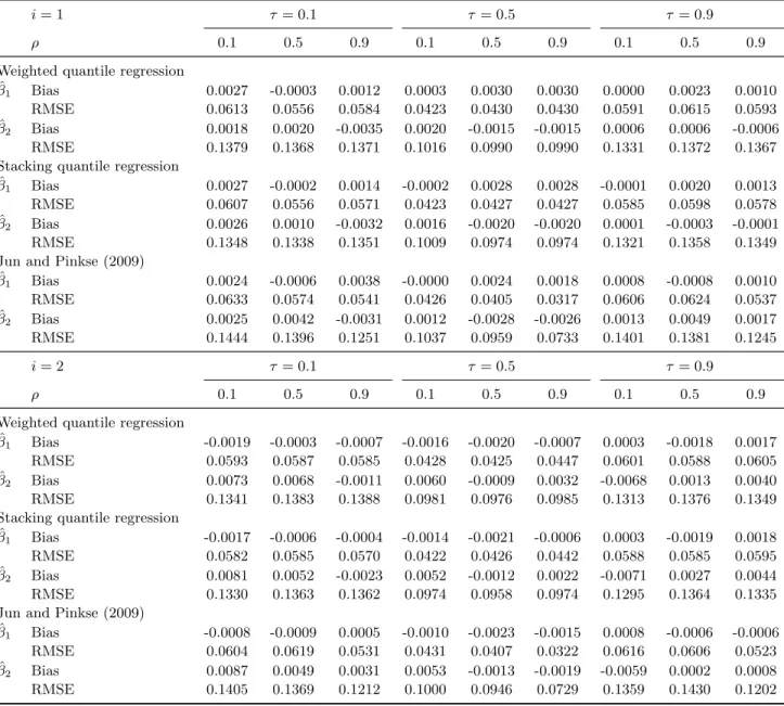
Table 3: Bias and RMSE for different error correlation with homoskedasticity

i = 1 τ = 0.1 τ = 0.5 τ = 0.9 ρ 0.1 0.5 0.9 0.1 0.5 0.9 0.1 0.5 0.9 Weighted quantile regression

ˆ β1 Bias 0.0027 -0.0003 0.0012 0.0003 0.0030 0.0030 0.0000 0.0023 0.0010 RMSE 0.0613 0.0556 0.0584 0.0423 0.0430 0.0430 0.0591 0.0615 0.0593 ˆ β2 Bias 0.0018 0.0020 -0.0035 0.0020 -0.0015 -0.0015 0.0006 0.0006 -0.0006 RMSE 0.1379 0.1368 0.1371 0.1016 0.0990 0.0990 0.1331 0.1372 0.1367 Stacking quantile regression

ˆ β1 Bias 0.0027 -0.0002 0.0014 -0.0002 0.0028 0.0028 -0.0001 0.0020 0.0013 RMSE 0.0607 0.0556 0.0571 0.0423 0.0427 0.0427 0.0585 0.0598 0.0578 ˆ β2 Bias 0.0026 0.0010 -0.0032 0.0016 -0.0020 -0.0020 0.0001 -0.0003 -0.0001 RMSE 0.1348 0.1338 0.1351 0.1009 0.0974 0.0974 0.1321 0.1358 0.1349 Jun and Pinkse (2009)

ˆ β1 Bias 0.0024 -0.0006 0.0038 -0.0000 0.0024 0.0018 0.0008 -0.0008 0.0010 RMSE 0.0633 0.0574 0.0541 0.0426 0.0405 0.0317 0.0606 0.0624 0.0537 ˆ β2 Bias 0.0025 0.0042 -0.0031 0.0012 -0.0028 -0.0026 0.0013 0.0049 0.0017 RMSE 0.1444 0.1396 0.1251 0.1037 0.0959 0.0733 0.1401 0.1381 0.1245 i = 2 τ = 0.1 τ = 0.5 τ = 0.9 ρ 0.1 0.5 0.9 0.1 0.5 0.9 0.1 0.5 0.9 Weighted quantile regression

ˆ β1 Bias -0.0019 -0.0003 -0.0007 -0.0016 -0.0020 -0.0007 0.0003 -0.0018 0.0017 RMSE 0.0593 0.0587 0.0585 0.0428 0.0425 0.0447 0.0601 0.0588 0.0605 ˆ β2 Bias 0.0073 0.0068 -0.0011 0.0060 -0.0009 0.0032 -0.0068 0.0013 0.0040 RMSE 0.1341 0.1383 0.1388 0.0981 0.0976 0.0985 0.1313 0.1376 0.1349 Stacking quantile regression

ˆ β1 Bias -0.0017 -0.0006 -0.0004 -0.0014 -0.0021 -0.0006 0.0003 -0.0019 0.0018 RMSE 0.0582 0.0585 0.0570 0.0422 0.0426 0.0442 0.0588 0.0585 0.0595 ˆ β2 Bias 0.0081 0.0052 -0.0023 0.0052 -0.0012 0.0022 -0.0071 0.0027 0.0044 RMSE 0.1330 0.1363 0.1362 0.0974 0.0958 0.0974 0.1295 0.1364 0.1335 Jun and Pinkse (2009)

ˆ β1 Bias -0.0008 -0.0009 0.0005 -0.0010 -0.0023 -0.0015 0.0008 -0.0006 -0.0006 RMSE 0.0604 0.0619 0.0531 0.0431 0.0407 0.0322 0.0616 0.0606 0.0523 ˆ β2 Bias 0.0087 0.0049 0.0031 0.0053 -0.0013 -0.0019 -0.0059 0.0002 0.0008 RMSE 0.1405 0.1369 0.1212 0.1000 0.0946 0.0729 0.1359 0.1430 0.1202 Notes: T = 100, (e1t, e2t) ∼ BN (0, 0, 1, 1, ρ) , replication=1000.

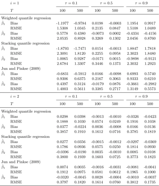
Table 4: Bias and RMSE for different sample size with heteroskedasticity

i = 1 τ = 0.1 τ = 0.5 τ = 0.9 T 100 500 100 500 100 500 Weighted quantile regression

ˆ β1 Bias -1.1977 -0.9784 0.0198 -0.0003 1.1954 0.9917 RMSE 1.5308 1.0345 0.2135 0.0847 1.5108 1.0489 ˆ β2 Bias 0.5778 0.4380 -0.0073 0.0002 -0.4334 -0.4156 RMSE 2.0535 0.8928 0.3269 0.1302 2.0456 0.8760 Stacking quantile regression

ˆ β1 Bias -1.8793 -1.7471 0.0154 -0.0013 1.8847 1.7818 RMSE 2.3091 1.8120 0.2255 0.0958 2.3023 1.8480 ˆ β2 Bias 1.0065 0.9287 -0.0171 0.0015 -0.9898 -0.9121 RMSE 2.6784 1.3307 0.3446 0.1373 2.3032 1.2923 Jun and Pinkse (2009)

ˆ β1 Bias -0.6831 -0.5912 0.0166 -0.0098 0.6993 0.5740 RMSE 0.9306 0.6375 0.2167 0.3063 0.9333 0.6210 ˆ β2 Bias 0.4397 0.3124 -0.0179 0.0876 -0.3661 -0.2982 RMSE 1.4003 0.5611 0.3385 0.2717 1.3149 0.5573 i = 2 τ = 0.1 τ = 0.5 τ = 0.9 T 100 500 100 500 100 500 Weighted quantile regression

ˆ β1 Bias 0.0298 0.0398 -0.0013 -0.0010 -0.0326 -0.0423 RMSE 0.1888 0.1030 0.0574 0.0249 0.1916 0.1038 ˆ β2 Bias 0.0377 -0.0224 0.0036 -0.0008 0.0166 0.0136 RMSE 0.3857 0.1910 0.1612 0.0716 0.3785 0.1819 Stacking quantile regression

ˆ β1 Bias 0.0277 0.0356 -0.0015 -0.0012 -0.0297 -0.0369 RMSE 0.1786 0.0936 0.0575 0.0250 0.1814 0.0930 ˆ β2 Bias -0.0396 -0.0190 0.0035 -0.0010 0.0085 0.0108 RMSE 0.3800 0.1939 0.1603 0.0725 0.3773 0.1823 Jun and Pinkse (2009)

ˆ β1 Bias 0.0074 0.0035 -0.0016 -0.0031 -0.0081 -0.0041 RMSE 0.1912 0.0975 0.0581 0.0612 0.1965 0.1000 ˆ β2 Bias -0.0320 -0.0045 0.0028 -0.0004 -0.0010 -0.0037 RMSE 0.3797 0.1820 0.1614 0.0760 0.3812 0.1735 Notes: The heteroskedastic form for i = 1 is h1(Xt) = exp(|x

0 t1β1+ x

0

t2β2|/10). The heteroskedastic form for i = 2 is h2(Xt) = 1+3exp(−(x

0 t1β1+x

0

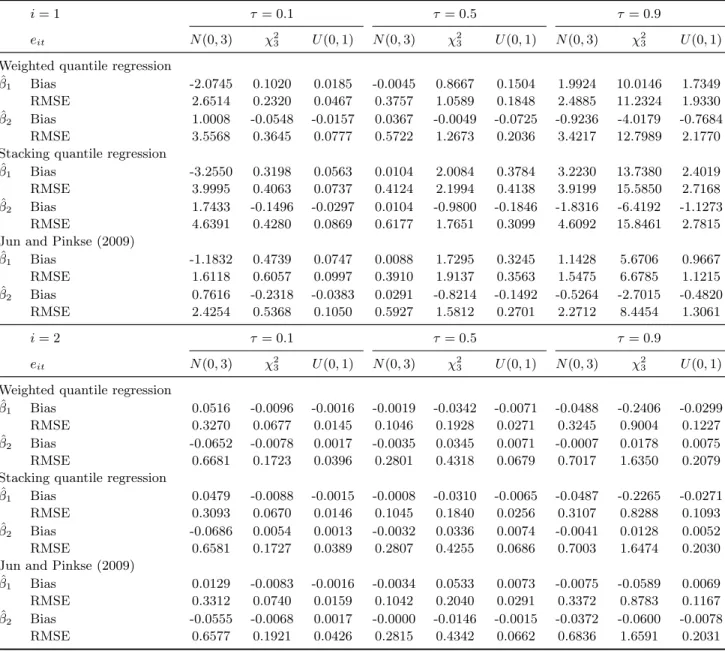
Table 5: Bias and RMSE for different error distribution with heteroskedasticity

i = 1 τ = 0.1 τ = 0.5 τ = 0.9

eit N (0, 3) χ23 U (0, 1) N (0, 3) χ23 U (0, 1) N (0, 3) χ23 U (0, 1) Weighted quantile regression

ˆ β1 Bias -2.0745 0.1020 0.0185 -0.0045 0.8667 0.1504 1.9924 10.0146 1.7349 RMSE 2.6514 0.2320 0.0467 0.3757 1.0589 0.1848 2.4885 11.2324 1.9330 ˆ β2 Bias 1.0008 -0.0548 -0.0157 0.0367 -0.0049 -0.0725 -0.9236 -4.0179 -0.7684 RMSE 3.5568 0.3645 0.0777 0.5722 1.2673 0.2036 3.4217 12.7989 2.1770 Stacking quantile regression

ˆ β1 Bias -3.2550 0.3198 0.0563 0.0104 2.0084 0.3784 3.2230 13.7380 2.4019 RMSE 3.9995 0.4063 0.0737 0.4124 2.1994 0.4138 3.9199 15.5850 2.7168 ˆ β2 Bias 1.7433 -0.1496 -0.0297 0.0104 -0.9800 -0.1846 -1.8316 -6.4192 -1.1273 RMSE 4.6391 0.4280 0.0869 0.6177 1.7651 0.3099 4.6092 15.8461 2.7815 Jun and Pinkse (2009)

ˆ β1 Bias -1.1832 0.4739 0.0747 0.0088 1.7295 0.3245 1.1428 5.6706 0.9667 RMSE 1.6118 0.6057 0.0997 0.3910 1.9137 0.3563 1.5475 6.6785 1.1215 ˆ β2 Bias 0.7616 -0.2318 -0.0383 0.0291 -0.8214 -0.1492 -0.5264 -2.7015 -0.4820 RMSE 2.4254 0.5368 0.1050 0.5927 1.5812 0.2701 2.2712 8.4454 1.3061 i = 2 τ = 0.1 τ = 0.5 τ = 0.9 eit N (0, 3) χ23 U (0, 1) N (0, 3) χ 2 3 U (0, 1) N (0, 3) χ 2 3 U (0, 1) Weighted quantile regression

ˆ β1 Bias 0.0516 -0.0096 -0.0016 -0.0019 -0.0342 -0.0071 -0.0488 -0.2406 -0.0299 RMSE 0.3270 0.0677 0.0145 0.1046 0.1928 0.0271 0.3245 0.9004 0.1227 ˆ β2 Bias -0.0652 -0.0078 0.0017 -0.0035 0.0345 0.0071 -0.0007 0.0178 0.0075 RMSE 0.6681 0.1723 0.0396 0.2801 0.4318 0.0679 0.7017 1.6350 0.2079 Stacking quantile regression

ˆ β1 Bias 0.0479 -0.0088 -0.0015 -0.0008 -0.0310 -0.0065 -0.0487 -0.2265 -0.0271 RMSE 0.3093 0.0670 0.0146 0.1045 0.1840 0.0256 0.3107 0.8288 0.1093 ˆ β2 Bias -0.0686 0.0054 0.0013 -0.0032 0.0336 0.0074 -0.0041 0.0128 0.0052 RMSE 0.6581 0.1727 0.0389 0.2807 0.4255 0.0686 0.7003 1.6474 0.2030 Jun and Pinkse (2009)

ˆ β1 Bias 0.0129 -0.0083 -0.0016 -0.0034 0.0533 0.0073 -0.0075 -0.0589 0.0069 RMSE 0.3312 0.0740 0.0159 0.1042 0.2040 0.0291 0.3372 0.8783 0.1167 ˆ β2 Bias -0.0555 -0.0068 0.0017 -0.0000 -0.0146 -0.0015 -0.0372 -0.0600 -0.0078 RMSE 0.6577 0.1921 0.0426 0.2815 0.4342 0.0662 0.6836 1.6591 0.2031 Notes: The heteroskedastic form for i = 1 is h1(Xt) = exp(|x

0 t1β1+ x

0

t2β2|/10). The heteroskedastic form for i = 2 is h2(Xt) = 1 + 3exp(−(x

0 t1β1+ x

0

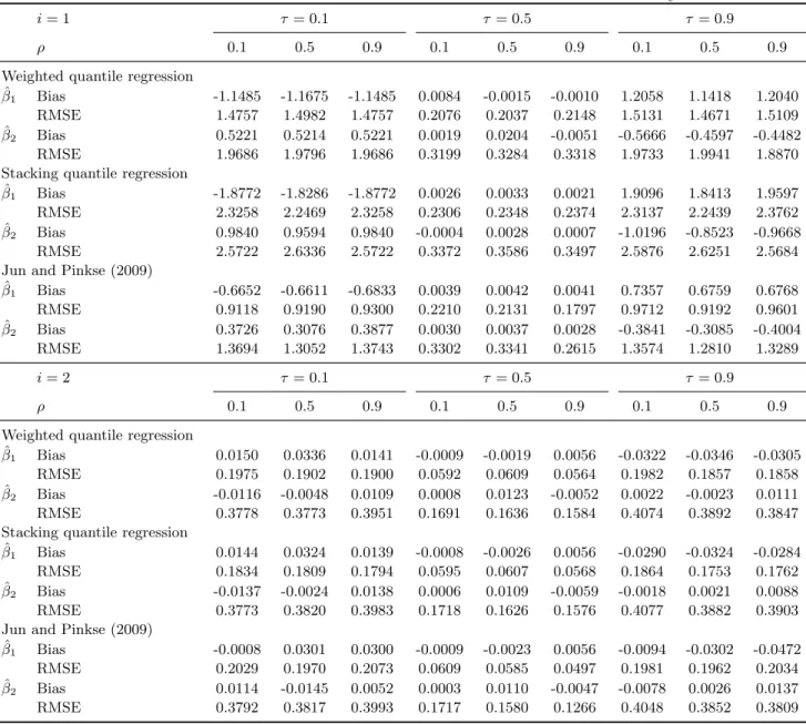
Table 6: Bias and RMSE for different error correlation with heteroskedasticity

i = 1 τ = 0.1 τ = 0.5 τ = 0.9 ρ 0.1 0.5 0.9 0.1 0.5 0.9 0.1 0.5 0.9 Weighted quantile regression

ˆ β1 Bias -1.1485 -1.1675 -1.1485 0.0084 -0.0015 -0.0010 1.2058 1.1418 1.2040 RMSE 1.4757 1.4982 1.4757 0.2076 0.2037 0.2148 1.5131 1.4671 1.5109 ˆ β2 Bias 0.5221 0.5214 0.5221 0.0019 0.0204 -0.0051 -0.5666 -0.4597 -0.4482 RMSE 1.9686 1.9796 1.9686 0.3199 0.3284 0.3318 1.9733 1.9941 1.8870 Stacking quantile regression

ˆ β1 Bias -1.8772 -1.8286 -1.8772 0.0026 0.0033 0.0021 1.9096 1.8413 1.9597 RMSE 2.3258 2.2469 2.3258 0.2306 0.2348 0.2374 2.3137 2.2439 2.3762 ˆ β2 Bias 0.9840 0.9594 0.9840 -0.0004 0.0028 0.0007 -1.0196 -0.8523 -0.9668 RMSE 2.5722 2.6336 2.5722 0.3372 0.3586 0.3497 2.5876 2.6251 2.5684 Jun and Pinkse (2009)

ˆ β1 Bias -0.6652 -0.6611 -0.6833 0.0039 0.0042 0.0041 0.7357 0.6759 0.6768 RMSE 0.9118 0.9190 0.9300 0.2210 0.2131 0.1797 0.9712 0.9192 0.9601 ˆ β2 Bias 0.3726 0.3076 0.3877 0.0030 0.0037 0.0028 -0.3841 -0.3085 -0.4004 RMSE 1.3694 1.3052 1.3743 0.3302 0.3341 0.2615 1.3574 1.2810 1.3289 i = 2 τ = 0.1 τ = 0.5 τ = 0.9 ρ 0.1 0.5 0.9 0.1 0.5 0.9 0.1 0.5 0.9 Weighted quantile regression

ˆ β1 Bias 0.0150 0.0336 0.0141 -0.0009 -0.0019 0.0056 -0.0322 -0.0346 -0.0305 RMSE 0.1975 0.1902 0.1900 0.0592 0.0609 0.0564 0.1982 0.1857 0.1858 ˆ β2 Bias -0.0116 -0.0048 0.0109 0.0008 0.0123 -0.0052 0.0022 -0.0023 0.0111 RMSE 0.3778 0.3773 0.3951 0.1691 0.1636 0.1584 0.4074 0.3892 0.3847 Stacking quantile regression

ˆ β1 Bias 0.0144 0.0324 0.0139 -0.0008 -0.0026 0.0056 -0.0290 -0.0324 -0.0284 RMSE 0.1834 0.1809 0.1794 0.0595 0.0607 0.0568 0.1864 0.1753 0.1762 ˆ β2 Bias -0.0137 -0.0024 0.0138 0.0006 0.0109 -0.0059 -0.0018 0.0021 0.0088 RMSE 0.3773 0.3820 0.3983 0.1718 0.1626 0.1576 0.4077 0.3882 0.3903 Jun and Pinkse (2009)

ˆ β1 Bias -0.0008 0.0301 0.0300 -0.0009 -0.0023 0.0056 -0.0094 -0.0302 -0.0472 RMSE 0.2029 0.1970 0.2073 0.0609 0.0585 0.0497 0.1981 0.1962 0.2034 ˆ β2 Bias 0.0114 -0.0145 0.0052 0.0003 0.0110 -0.0047 -0.0078 0.0026 0.0137 RMSE 0.3792 0.3817 0.3993 0.1717 0.1580 0.1266 0.4048 0.3852 0.3809 Notes: The heteroskedastic form for i = 1 is h1(Xt) = exp(|x

0 t1β1+ x

0

t2β2|/10). The heteroskedastic form for i = 2 is h2(Xt) = 1 + 3exp(−(x

0 t1β1+ x

0

t2β2+ 10)2/100). T = 100, (e1t, e2t) ∼ BN (0, 0, 1, 1, ρ) , replication=1000.

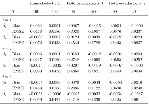
Table 7: Bias and RMSE in the SUR model with three equations

Homoskedasticity Heteroskedasticity 1 Heteroskedasticity 2 T 100 500 100 500 100 500 i = 1 ˆ β1 Bias 0.0004 0.0001 0.0067 -0.0016 0.0004 -0.0000 RMSE 0.0433 0.0180 0.3020 0.1007 0.0576 0.0237 ˆ β2 Bias -0.0006 0.0007 0.0124 0.0039 -0.0021 0.0023 RMSE 0.0972 0.0433 0.4544 0.1786 0.1445 0.0637 i = 2 ˆ β1 Bias 0.0006 0.0001 0.0153 -0.0012 -0.0004 0.0003 RMSE 0.0417 0.0190 0.2748 0.1060 0.0565 0.0252 ˆ β2 Bias -0.0013 -0.0002 0.0207 -0.0019 -0.0007 -0.0003 RMSE 0.0960 0.0428 0.4860 0.1821 0.1403 0.0634 i = 3 ˆ β1 Bias -0.0035 0.0008 0.0079 0.0043 -0.0053 0.0010 RMSE 0.0433 0.0188 0.2885 0.1122 0.0590 0.0248 ˆ β2 Bias -0.0028 -0.0006 -0.0025 0.0032 -0.0064 -0.0017 RMSE 0.0959 0.0424 0.4718 0.1836 0.1425 0.0611 Notes: eit∼ N (0, 1) , τ = 0.5 , ρ = 0 , replication=1000.

Table 8: Bias and RMSE for different error distribution for three equations on

RDQR

Homoskedasticity Heteroskedasticity 1 Heteroskedasticity 2 eit N (0, 3) χ23 U (0, 1) N (0, 3) χ23 U (0, 1) N (0, 3) χ23 U (0, 1) i = 1 ˆ β1 Bias -0.0010 0.0017 -0.0001 -0.0158 3.6987 0.6649 -0.0016 -0.0898 -0.0156 RMSE 0.0716 0.0862 0.0155 0.4811 4.1105 0.7307 0.0961 0.1771 0.0276 ˆ β2 Bias 0.0125 -0.0037 0.0014 0.0511 -1.9517 -0.3461 0.0188 0.0425 0.0105 RMSE 0.1736 0.2086 0.0374 0.8073 3.4659 0.6208 0.2641 0.3712 0.0585 i = 2 ˆ β1 Bias 0.0028 0.0034 -0.0009 0.0220 3.9043 0.6941 0.0027 -0.0985 -0.0158 RMSE 0.0729 0.0896 0.0162 0.4779 4.3211 0.7690 0.0990 0.1812 0.0271 ˆ β2 Bias -0.0071 0.0001 -0.0008 -0.0469 -2.0155 -0.3430 -0.0088 0.0522 0.0094 RMSE 0.1691 0.2050 0.0389 0.8186 3.4652 0.6069 0.2476 0.3916 0.0558 i = 3 ˆ β1 Bias 0.0025 0.0017 0.0006 0.0144 3.7128 0.6821 0.0009 -0.1027 -0.0162 RMSE 0.0761 0.0871 0.0159 0.5293 4.1513 0.7548 0.1009 0.1842 0.0285 ˆ β2 Bias 0.0003 0.0101 -0.0001 -0.0241 -1.8736 -0.3454 0.0007 0.0334 0.0068 RMSE 0.1637 0.2092 0.0360 0.8375 3.4150 0.6299 0.2430 0.3709 0.0550 Notes: T = 100 , τ = 0.5 , ρ = 0 , replication=1000.

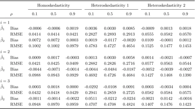
Table 9: Bias and RMSE for different error correlation for three equations on RDQR

Homoskedasticity Heteroskedasticity 1 Heteroskedasticity 2 ρ 0.1 0.5 0.9 0.1 0.5 0.9 0.1 0.5 0.9 i = 1 ˆ β1 Bias -0.0006 -0.0006 0.0019 0.0036 0.0030 0.0085 -0.0009 0.0013 0.0018 RMSE 0.0414 0.0414 0.0421 0.2827 0.2893 0.2913 0.0555 0.0582 0.0570 ˆ β2 Bias 0.0072 0.0072 0.0003 0.0019 -0.0117 -0.0020 0.0109 -0.0001 0.0012 RMSE 0.1002 0.1002 0.0979 0.4783 0.4727 0.4654 0.1525 0.1477 0.1453 i = 2 ˆ β1 Bias 0.0009 0.0017 -0.0003 0.0013 0.0030 0.0058 0.0014 -0.0021 -0.0007 RMSE 0.0421 0.0425 0.0409 0.2882 0.2826 0.2716 0.0577 0.0563 0.0544 ˆ β2 Bias -0.0044 -0.0071 -0.0014 -0.0044 -0.0484 -0.0187 -0.0052 -0.0039 -0.0027 RMSE 0.0988 0.0943 0.0929 0.4692 0.4726 0.4684 0.1427 0.1468 0.1390 i = 3 ˆ β1 Bias 0.0003 0.0018 0.0000 -0.0292 -0.0108 0.0091 0.0003 -0.0034 0.0004 RMSE 0.0432 0.0418 0.0429 0.2941 0.2859 0.2725 0.0582 0.0584 0.0575 ˆ β2 Bias -0.0011 -0.0014 -0.0022 0.0511 -0.0212 -0.0234 -0.0021 0.0142 -0.0016 RMSE 0.0948 0.0970 0.0959 0.4707 0.4708 0.4824 0.1407 0.1476 0.1423 Notes: T = 100 , τ = 0.5 , (e1t, e2t) ∼ BN (0, 0, 1, 1, ρ) , replication=1000.

Table 10: Bias and RMSE for different sample size for five equations on RDQR

Homoskedasticity Heteroskedasticity 1 Heteroskedasticity 2 T 100 500 100 500 100 500 i = 1 ˆ β1 Bias -0.0011 -0.0005 0.0023 0.0047 -0.0011 -0.0013 RMSE 0.0412 0.0185 0.4909 0.1457 0.0537 0.0235 ˆ β2 Bias 0.0067 0.0005 -0.0106 -0.0083 0.0044 -0.0028 RMSE 0.0955 0.0424 0.8265 0.2793 0.1243 0.0564 i = 2 ˆ β1 Bias 0.0023 -0.0000 0.0062 0.0036 0.0025 0.0000 RMSE 0.0443 0.0186 0.4708 0.1520 0.0533 0.0236 ˆ β2 Bias 0.0007 -0.0007 -0.0044 0.0016 -0.0018 0.0031 RMSE 0.0984 0.0431 0.8226 0.2725 0.1267 0.0578 i = 3 ˆ β1 Bias -0.0014 -0.0009 -0.0462 0.0020 0.0004 0.0008 RMSE 0.0424 0.0192 0.5005 0.1523 0.0524 0.0228 ˆ β2 Bias -0.0051 0.0004 0.0247 -0.0027 -0.0063 -0.0012 RMSE 0.1016 0.0452 0.8649 0.2809 0.1275 0.0567 i = 4 ˆ β1 Bias -0.0005 0.0002 0.0222 0.0042 0.0021 0.0004 RMSE 0.0441 0.0182 0.4918 0.1577 0.0560 0.0238 ˆ β2 Bias -0.0005 0.0016 0.0014 -0.0035 0.0013 -0.0014 RMSE 0.0995 0.0434 0.9038 0.2813 0.1285 0.0572 i = 5 ˆ β1 Bias -0.0010 -0.0006 -0.0278 -0.0023 -0.0014 -0.0016 RMSE 0.0418 0.0188 0.5047 0.1545 0.0527 0.0237 ˆ β2 Bias -0.0033 0.0002 0.0347 -0.0068 0.0033 0.0010 RMSE 0.0976 0.0418 0.8402 0.2773 0.1301 0.0544 Notes: eit∼ N (0, 1) , τ = 0.5 , ρ = 0 , replication=1000.

Table 11: Bias and RMSE for different error distribution for five equations on RDQR

Homoskedasticity Heteroskedasticity 1 Heteroskedasticity 2 eit N (0, 3) χ23 U (0, 1) N (0, 3) χ 2 3 U (0, 1) N (0, 3) χ 2 3 U (0, 1) i = 1 ˆ β1 Bias -0.0018 0.0020 -0.0007 0.0023 12.0246 2.2043 -0.0024 -0.0897 -0.0157 RMSE 0.0711 0.0846 0.0164 0.8721 13.8380 2.5299 0.0895 0.1610 0.0255 ˆ β2 Bias -0.0010 -0.0024 -0.0010 0.0371 -5.5198 -1.0310 0.0016 0.0411 0.0097 RMSE 0.1713 0.2035 0.0362 1.5737 12.3472 2.1311 0.2176 0.3151 0.0488 i = 2 ˆ β1 Bias 0.0000 -0.0019 -0.0003 0.0058 12.4915 2.1290 0.0001 -0.0930 -0.0153 RMSE 0.0726 0.0859 0.0162 0.9033 14.5672 2.4466 0.0908 0.1606 0.0258 ˆ β2 Bias -0.0045 -0.0054 0.0025 0.1412 -5.9430 -1.1250 -0.0069 0.0386 0.0051 RMSE 0.1656 0.2112 0.0366 1.5777 12.1974 2.1772 0.2121 0.3180 0.0487 i = 3 ˆ β1 Bias -0.0000 -0.0023 -0.0003 -0.0071 12.3931 2.1597 -0.0002 -0.0896 -0.0160 RMSE 0.0731 0.0920 0.0160 0.9092 14.3181 2.4882 0.0925 0.1601 0.0258 ˆ β2 Bias 0.0023 -0.0101 0.0005 -0.0267 -6.3941 -0.9930 0.0029 0.0715 0.0085 RMSE 0.1720 0.2006 0.0375 1.4581 12.5587 2.1182 0.2195 0.3039 0.0485 i = 4 ˆ β1 Bias -0.0031 -0.0028 0.0005 -0.0200 12.5119 2.1433 -0.0030 -0.0888 -0.0146 RMSE 0.0746 0.0908 0.0167 0.8823 14.4012 2.4677 0.0935 0.1582 0.0248 ˆ β2 Bias 0.0040 0.0092 0.0001 -0.0253 -6.1826 -1.0128 0.0020 0.0359 0.0075 RMSE 0.1703 0.2017 0.0370 1.5708 12.5563 2.1759 0.2215 0.2998 0.0494 i = 5 ˆ β1 Bias 0.0035 -0.0001 -0.0005 0.0165 12.5495 2.1569 0.0046 -0.0882 -0.0141 RMSE 0.0750 0.0882 0.0161 0.8363 14.6029 2.5037 0.0948 0.1528 0.0247 ˆ β2 Bias 0.0045 0.0023 0.0005 0.0119 -6.5410 -1.1390 0.0049 0.0386 0.0112 RMSE 0.1653 0.2008 0.0389 1.5814 13.0492 2.2205 0.2185 0.3045 0.0485 Notes: T = 100 , τ = 0.5 , ρ = 0 , replication=1000.

Table 12: Bias and RMSE for different error correlation for five equations on RDQR

Homoskedasticity Heteroskedasticity 1 Heteroskedasticity 2 ρ 0.1 0.5 0.9 0.1 0.5 0.9 0.1 0.5 0.9 i = 1 ˆ β1 Bias -0.0010 0.0010 0.0010 0.0067 0.0208 0.0142 -0.0014 0.0009 0.0011 RMSE 0.0410 0.0423 0.0439 0.5057 0.5004 0.4837 0.0517 0.0529 0.0537 ˆ β2 Bias -0.0006 0.0026 -0.0006 0.0441 0.0296 0.0002 0.0009 0.0044 0.0019 RMSE 0.0989 0.0959 0.0973 0.9156 0.9036 0.8421 0.1256 0.1181 0.1309 i = 2 ˆ β1 Bias -0.0002 0.0013 0.0026 -0.0180 0.0126 0.0108 -0.0008 0.0020 0.0010 RMSE 0.0416 0.0412 0.0433 0.5265 0.4914 0.4701 0.0524 0.0527 0.0546 ˆ β2 Bias -0.0026 0.0041 0.0003 -0.0285 -0.0102 0.0088 -0.0032 0.0053 -0.0065 RMSE 0.0963 0.0996 0.0960 0.8761 0.8523 0.8783 0.1231 0.1290 0.1255 i = 3 ˆ β1 Bias 0.0001 0.0009 -0.0014 -0.0190 0.0166 -0.0270 -0.0003 0.0009 0.0022 RMSE 0.0424 0.0439 0.0432 0.5202 0.4726 0.4792 0.0533 0.0567 0.0545 ˆ β2 Bias 0.0007 -0.0019 -0.0010 0.0173 0.0373 0.0088 0.0010 -0.0028 0.0001 RMSE 0.0989 0.0964 0.0978 0.9377 0.8027 0.8340 0.1265 0.1234 0.1268 i = 4 ˆ β1 Bias -0.0015 -0.0007 0.0004 -0.0231 0.0386 0.0073 -0.0022 -0.0004 -0.0002 RMSE 0.0429 0.0427 0.0412 0.5027 0.4863 0.4478 0.0542 0.0536 0.0550 ˆ β2 Bias -0.0000 -0.0044 0.0118 0.0134 -0.0294 0.0614 -0.0005 -0.0052 -0.0057 RMSE 0.0957 0.0990 0.0975 0.9288 0.8726 0.8323 0.1250 0.1269 0.1251 i = 5 ˆ β1 Bias 0.0022 -0.0002 -0.0004 0.0103 -0.0175 0.0072 0.0032 -0.0005 -0.0017 RMSE 0.0435 0.0422 0.0419 0.5410 0.5075 0.4957 0.0547 0.0537 0.0539 ˆ β2 Bias 0.0038 0.0041 0.0013 0.0006 0.0218 -0.0336 0.0039 0.0063 -0.0013 RMSE 0.1011 0.0970 0.1013 0.8823 0.8300 0.7983 0.1263 0.1271 0.1226 Notes: T = 100 , τ = 0.5 , (e1t, e2t) ∼ BN (0, 0, 1, 1, ρ) , replication=1000.

Table 13: Descriptive statistics

Mean First Median Third Standard Minimum Maximum quartile quartile deviation

Australian dollar spot 1.3712 1.1093 1.3187 1.5783 0.3132 0.9104 2.0479 forward 1.3735 1.1160 1.3220 1.5765 0.3127 0.9136 2.0500 Canadian dollar spot 1.2420 1.0329 1.1886 1.4739 0.2144 0.9489 1.6045 forward 1.2422 1.0334 1.1887 1.4734 0.2145 0.9495 1.6048 Danish krone spot 6.3021 5.5300 5.9073 6.9995 1.0884 4.7063 8.7967 forward 6.3015 5.5260 5.9081 6.9867 1.0885 4.7113 8.8041 Euro spot 0.8464 0.7430 0.7931 0.9421 0.1464 0.6311 1.1812 forward 0.8462 0.7425 0.7926 0.9400 0.1464 0.6317 1.1819 Japanese yen spot 105.4624 93.2675 109.1525 118.0700 15.0360 76.2500 133.8250 forward 105.2136 93.2523 108.7489 117.5664 14.9069 76.2271 133.6140 New Zealand dollar

spot 1.6433 1.3511 1.4954 1.9099 0.3811 1.1444 2.5195 forward 1.6466 1.3556 1.4967 1.9082 0.3806 1.1424 2.5116 Norwegian krone spot 6.7982 5.8801 6.5109 7.5328 1.1740 5.0818 9.3665 forward 6.8063 5.8890 6.5101 7.5576 1.1788 5.0948 9.3902 Swedish Krona spot 7.7756 6.8325 7.4840 8.4900 1.2481 5.9300 10.8854 forward 7.7753 6.8233 7.4887 8.4835 1.2480 5.9388 10.8892 Swiss franc spot 1.2611 1.0503 1.2322 1.4782 0.2608 0.7882 1.7981 forward 1.2592 1.0500 1.2280 1.4752 0.2598 0.7878 1.7966 UK pound spot 0.6059 0.5520 0.6195 0.6430 0.0616 0.4814 0.7110 forward 0.6063 0.5535 0.6199 0.6439 0.0615 0.4818 0.7118 Czechoslovakia koruna spot 25.4086 19.0382 22.8309 30.9600 7.4921 15.1721 41.1380 forward 25.4122 19.0466 22.7918 30.9932 7.5019 15.1896 41.0910 Hong Kong dollar

spot 7.7788 7.7582 7.7789 7.7991 0.0205 7.7438 7.8263 forward 7.7763 7.7568 7.7754 7.7972 0.0197 7.7408 7.8183

Table 14: Descriptive statistics@(continued)

Mean First Median Third Standard Minimum Maximum quartile quartile deviation

Hungarian forint spot 220.8675 195.1490 216.2053 238.9750 35.6554 149.0466 310.6299 forward 221.9705 195.8940 217.1385 240.7950 35.9471 149.7766 312.0149 Indian rupee spot 46.1539 43.8400 45.9175 47.9400 3.4378 39.3235 56.1575 forward 46.3113 43.8994 46.0763 48.1031 3.4995 39.3835 56.5025 Indonesia rupiah spot 9497.5760 8824.2500 9133.2500 9521.2500 857.3468 6825.0000 12025.0000 forward 9421.0920 9108.7500 9745.0000 9745.0000 778.3940 6860.5000 12195.0000 Kuwaiti dinar spot 0.2915 0.2818 0.2920 0.3020 0.0117 0.2650 0.3085 forward 0.2916 0.2818 0.2920 0.3022 0.0117 0.2646 0.3084 Mexican peso spot 11.1604 9.9500 10.9645 12.3386 1.4259 9.0128 15.0812 forward 11.2188 10.1074 11.0003 12.3685 1.4157 9.0608 15.1862 Philipine peso spot 47.8223 43.1250 47.8475 52.4250 5.3911 37.9750 56.3300 forward 47.9819 43.2030 47.9873 52.6540 5.4483 38.1485 56.6920 Saudi Arabian riyal

spot 3.7501 3.7502 3.7503 3.7505 0.0030 3.7150 3.7610 forward 3.7503 3.7499 3.7505 3.7515 0.0043 3.7050 3.7615 Singapore dollar

spot 1.5593 1.3983 1.6220 1.7250 0.1926 1.2023 1.8465 forward 1.5576 1.3986 1.6205 1.7221 0.1917 1.2021 1.8460 South African rand

spot 7.5523 6.6650 7.3038 8.0545 1.2791 5.6338 11.9950 forward 7.5954 6.6949 7.3582 8.1115 1.2950 5.6595 12.0800 Taiwan dollar spot 32.2387 31.0400 32.3885 33.3525 1.6929 28.6385 35.1050 forward 32.2025 30.9900 32.3485 33.3360 1.7034 28.6330 35.1690 Thai baht spot 37.0654 33.1300 37.5150 41.1675 4.6760 29.2850 45.7000 forward 37.1051 33.1485 37.5625 41.1925 4.6811 29.3405 45.8500 Turkish@lira spot 1.3366 1.2774 1.4308 1.5704 0.3860 0.3154 1.8886 forward 1.3224 1.2224 1.4482 1.5850 0.4123 0.3396 1.9019

Table 15: The normality test of future change in the spot exchange rate

Currencies Skewness Kurtosis J-B Currencies Skewness Kurtosis J-B

Australian dollar 0.8071 5.6374 68.1248∗∗∗ _{Hungarian forint 1.0904 6.2294 108.1913}∗∗∗

Canadian dollar 0.7185 7.0825 133.4633∗∗∗ _{Indian rupee 0.2803 5.9100 62.5741}∗∗∗

Danish krone 0.1606 3.7663 4.9191∗ Indonesia rupiah -0.7640 8.8201 257.9872∗∗∗

Euro 0.1687 3.7493 4.8119∗ Kuwaiti dinar 1.5351 17.0912 1481.915∗∗∗

Japanese yen 0.2598 3.2408 2.3374 Mexican peso 1.0996 7.2913 165.6672∗∗∗

New Zealand dollar 0.5008 4.8157 30.6374∗∗∗ Philipine peso 0.9358 6.5089 112.6827∗∗∗ Norwegian krone 0.5021 4.3095 19.4022∗∗∗ Saudi Arabian riyal 3.0610 65.3975 28007.8400∗∗∗

Swedish Krona 0.1393 3.4662 2.1019 Singapore dollar 0.8212 6.2256 93.3510∗∗∗

Swiss franc -0.1353 4.6977 21.0583∗∗∗ South African rand 0.5615 3.7348 12.8334∗∗∗

UK pound 0.4159 4.5760 22.6257∗∗∗ _{Taiwan dollar 0.0038 4.0598 8.0028}∗∗

Czechoslovakia koruna 0.4011 3.4786 6.2155∗∗ _{Thai baht 0.1764 4.1431 10.1963}∗∗∗

Hong Kong dollar -1.0816 10.3988 423.3821∗∗∗ _{Turkish@lira 2.0430 14.3612 1038.6280}∗∗∗

Notes: J-B is the statistic of Jarque-Bera normality test. ∗_,∗∗_and∗∗∗_{indicate the significant leves of 10%, 5%}

Table 16: Descriptive statistics–daily data

Mean First Median Third Standard Minimum Maximum quartile quartile deviation

Australian dollar spot 1.3683 1.1027 1.3225 1.5691 0.3085 0.9066 2.0648 forward 1.3708 1.1065 1.3240 1.5698 0.3080 0.9114 2.0710 Canadian dollar spot 1.2404 1.0289 1.1894 1.4727 0.2130 0.9161 1.6155 forward 1.2406 1.0293 1.1889 1.4725 0.2130 0.9161 1.6159 Danish krone spot 6.3039 5.5459 5.9166 6.9962 1.0773 4.6702 8.9828 forward 6.3034 5.5420 5.9129 6.9914 1.0774 4.6753 8.9742 Euro spot 0.8466 0.7446 0.7944 0.9410 0.1449 0.6258 1.2067 forward 0.8464 0.7442 0.7941 0.9396 0.1448 0.6266 1.2051 Japanese yen spot 105.4834 93.1050 108.4150 117.8050 14.9203 75.7600 134.8300 forward 105.2402 93.0801 108.0755 117.4260 14.7920 75.7329 134.6417 New Zealand dollar

spot 1.6394 1.3454 1.4975 1.8932 0.3744 1.1429 2.5400 forward 1.6427 1.3487 1.5014 1.8941 0.3740 1.1424 2.5526 Norwegian krone spot 6.7969 5.8752 6.5073 7.5305 1.1596 4.9584 9.5675 forward 6.8051 5.8820 6.5060 7.5617 1.1643 4.9733 9.5731 Swedish Krona spot 7.7726 6.8315 7.4775 8.4400 1.2288 5.8486 11.0318 forward 7.7744 6.8319 7.4515 8.3470 1.2338 5.9556 11.0718 Swiss franc spot 1.2608 1.0520 1.2338 1.4723 0.2579 0.7275 1.8090 forward 1.2589 1.0516 1.2308 1.4700 0.2570 0.7265 1.8174 UK pound spot 0.6067 0.5520 0.6196 0.6462 0.0613 0.4743 0.7316 forward 0.6072 0.5530 0.6198 0.6466 0.0612 0.4748 0.7320 Czechoslovakia koruna spot 25.3739 19.1077 22.9496 31.0475 7.4557 14.4979 42.0380 forward 25.3778 19.1170 22.9196 31.0825 7.4654 14.5149 41.9930 Hong Kong dollar

spot 7.7797 7.7592 7.7811 7.7993 0.0207 7.7098 7.8294 forward 7.7772 7.7577 7.7772 7.7976 0.0199 7.7033 7.8220 Hungarian forint

spot 221.0492 195.4264 216.2077 238.0915 35.1216 144.2562 317.1250 forward 222.1533 196.1369 217.1289 239.5915 35.4051 144.9563 318.5549

Table 17: Descriptive statistics–daily data (continued)

Mean First Median Third Standard Minimum Maximum quartile quartile deviation

Indian rupee spot 46.1923 43.8450 45.8100 47.9800 3.4490 39.2700 57.1862 forward 46.3518 43.9050 45.9225 48.1810 3.5112 39.3137 57.5662 Indonesia rupiah spot 9196.5420 8850.0000 9140.0000 9490.0000 844.7454 6575.0000 12150.0000 forward 9420.4410 9110.5000 9745.0000 9745.0000 763.5583 6665.0000 12360.0000 Kuwaiti dinar spot 0.2914 0.2821 0.2920 0.3021 0.0116 0.2644 0.3089 forward 0.2915 0.2822 0.2919 0.3023 0.0116 0.2643 0.3089 Mexican peso spot 11.1533 9.9650 10.9445 12.3810 1.4100 8.9280 15.3835 forward 11.2105 10.0764 10.9770 12.4089 1.3999 9.0045 15.4938 Philipine peso spot 47.7928 43.1850 47.6800 52.3750 5.3529 37.5500 56.4600 forward 47.9502 43.2750 47.8290 52.6060 5.4086 37.7415 56.8380 Saudi Arabian riyal

spot 3.7502 3.7502 3.7503 3.7505 0.0024 3.7110 3.7650 forward 3.7504 3.7498 3.7505 3.7514 0.0033 3.7015 3.7676 Singapore dollar

spot 1.5590 1.3944 1.6214 1.7234 0.1914 1.2008 1.8536 forward 1.5574 1.3943 1.6197 1.7203 0.1906 1.2004 1.8532 South African rand

spot 7.5917 6.6858 7.3350 8.1010 1.2935 5.6208 13.4700 forward 7.6351 6.7171 7.3734 8.1586 1.3102 5.6488 13.5650 Taiwan dollar spot 32.2366 30.9615 32.3945 33.4000 1.6857 28.5100 35.1800 forward 32.2043 30.8970 32.3545 33.4050 1.6945 28.5040 35.2850 Thai baht spot 37.0210 33.0000 37.4750 41.0695 4.6844 28.6150 45.8000 forward 37.0589 33.0495 37.5225 41.0900 4.6870 28.6725 46.1250 Turkish@lira spot 1.3436 1.2848 1.4315 1.5714 0.3831 0.3154 1.9181 forward 1.3268 1.2357 1.4447 1.5829 0.4104 0.3374 1.9304

Table 18: The normality test of future change in the spot exchange rate–daily data

Currencies Skewness Kurtosis J-B Currencies Skewness Kurtosis J-B

Australian dollar 0.4081 2.1147 225.9162∗∗∗ Hungarian forint 0.5948 2.8227 225.3814∗∗∗ Canadian dollar 0.2961 1.5662 374.8991∗∗∗ Indian rupee 0.7239 3.8335 434.7692∗∗∗ Danish krone 0.8348 2.5450 466.5587∗∗∗ Indonesia rupiah 0.3634 5.1192 781.9446∗∗∗

Euro 0.8262 2.5268 460.2508∗∗∗ _{Kuwaiti dinar -0.2894 2.2267 145.3651}∗∗∗

Japanese yen -0.4771 2.1231 261.6328∗∗∗ _{Mexican peso 0.3963 2.2228 191.9617}∗∗∗

New Zealand dollar 0.8063 2.4624 450.1979∗∗∗ _{Philipine peso 0.0131 1.7783 232.6352}∗∗∗

Norwegian krone 0.7150 2.4534 365.1591∗∗∗ _{Saudi Arabian riyal -8.5340 134.2793 2730340}∗∗∗

Swedish Krona 0.8410 2.8546 444.0083∗∗∗ Singapore dollar -0.3945 1.7823 327.9775∗∗∗ Swiss franc 0.3559 2.1335 195.9192∗∗∗ South African rand 1.1781 4.2100 1093.0010∗∗∗

UK pound -0.2714 2.0785 178.2072∗∗∗ Taiwan dollar -0.3025 2.2332 148.6346∗∗∗

Czechoslovakia koruna 0.6420 2.0443 399.1380∗∗∗ Thai baht 0.0277 1.7372 248.8927∗∗∗ Hong Kong dollar -0.0964 1.7289 257.5064∗∗∗ Turkish@lira -1.2280 3.7110 1018.4720∗∗∗

Notes: J-B is the statistic of Jarque-Bera normality test. ∗,∗∗and∗∗∗indicate the significant leves of 10%, 5% and 1% respectively.

科技部補助計畫衍生研發成果推廣資料表

日期:2015/10/22

科技部補助計畫

計畫名稱: 近似無關分量迴歸

計畫主持人: 林馨怡

計畫編號: 103-2410-H-004-014-

學門領域: 數理與數量方法

無研發成果推廣資料

103年度專題研究計畫研究成果彙整表

計畫主持人：

林馨怡

計畫編號：

103-2410-H-004-014-計畫名稱：

近似無關分量迴歸

成果項目

量化

單位

備註（質化說明

：如數個計畫共

同成果、成果列

為該期刊之封面

故事...等）

實際已達成

數（被接受

或已發表）

預期總達成

數（含實際

已達成數）

本計畫實

際貢獻百

分比

國內

論文著作

期刊論文

0

0

100%

篇

研究報告/技術報告

1

1

100%

研討會論文

0

0

100%

專書

0

0

100%

章/本

專利

申請中件數

0

0

100%

件

已獲得件數

0

0

100%

技術移轉

件數

0

0

100%

件

權利金

0

0

100%

千元

參與計畫人力

（本國籍）

碩士生

1

1

100%

人次

博士生

0

0

100%

博士後研究員

0

0

100%

專任助理

1

1

100%

國外

論文著作

期刊論文

0

1

100%

篇

研究報告/技術報告

0

0

100%

研討會論文

0

0

100%

專書

0

0

100%

章/本

專利

申請中件數

0

0

100%

件

已獲得件數

0

0

100%

技術移轉

件數

0

0

100%

件

權利金

0

0

100%

千元

參與計畫人力

（外國籍）

碩士生

0

0

100%

人次

博士生

0

0

100%

博士後研究員

0

0

100%

專任助理

0

0

100%

其他成果

（無法以量化表達之

成果如辦理學術活動

、獲得獎項、重要國

際合作、研究成果國

際影響力及其他協助

產業技術發展之具體

效益事項等，請以文

無。

成果項目

量化

名稱或內容性質簡述

科

教

處

計

畫

加

填

項

目

測驗工具(含質性與量性)

0

課程/模組

0

電腦及網路系統或工具

0

教材

0

舉辦之活動/競賽

0

研討會/工作坊

0

電子報、網站

0

計畫成果推廣之參與（閱聽）人數

0

科技部補助專題研究計畫成果報告自評表

請就研究內容與原計畫相符程度、達成預期目標情況、研究成果之學術或應用價

值（簡要敘述成果所代表之意義、價值、影響或進一步發展之可能性）、是否適

合在學術期刊發表或申請專利、主要發現或其他有關價值等，作一綜合評估。

1. 請就研究內容與原計畫相符程度、達成預期目標情況作一綜合評估

■達成目標

□未達成目標（請說明，以100字為限）

　　□實驗失敗

　　□因故實驗中斷

　　□其他原因

說明：

2. 研究成果在學術期刊發表或申請專利等情形：

論文：□已發表 □未發表之文稿 ■撰寫中 □無

專利：□已獲得 □申請中 ■無

技轉：□已技轉 □洽談中 ■無

其他：（以100字為限）

3. 請依學術成就、技術創新、社會影響等方面，評估研究成果之學術或應用價值

（簡要敘述成果所代表之意義、價值、影響或進一步發展之可能性）（以

500字為限）

本研究計劃提出之方法可以應用到各種總體或產業實證。另外，本計劃對遠期

外匯不偏性假說此一議題的實證研究，提供更完整的分析。