Blind and Semiblind Detections of
OFDM Signals in Fading Channels
Ming-Xian Chang, Member, IEEE, and Yu T. Su, Member, IEEE
Abstract—This paper considers the problem of blind joint
channel estimation and data detection for orthogonal fre-quency-division multiplexing (OFDM) systems in a fading environment. Employing a regression model for a time-varying channel, we convert the problem into one that finds the data sequencex whose associated least-squares (LS) channel estimate z(x) is closest to the space of some regression curves (surfaces). We apply the branch-and-bound principle to solve the nonlinear integer programming problem associated with finding the curve that fits a subchannel in the LS sense. A recursive formula for fast metric update is obtained by exploiting the intrinsic characteristic of our objective function. The impacts of reordering the data sequence and selective detection are addressed. By employing a preferred order along with a selective detection method, we greatly reduce the detector complexity while giving up little performance loss. Both the complete and the reduced-complexity algorithms can be used for blind and semiblind detections of OFDM signals in a subchannel-by-subchannel manner. To further reduce the com-plexity and exploit the frequency-domain channel correlation, we suggest a two-stage approach that detects a few selected positions in some subchannels first, and then, treating the detected symbols as pilots, determines the remaining symbols within a properly chosen time-frequency block by a two-dimensional model-based pilot-assisted algorithm. The proposed methods do not require the information of the channel statistics like signal-to-noise ratio or channel correlation function. Performance of differential modulations like differential quaternary phase-shift keying and STAR 16-ary quadrature amplitude modulation are provided. Both blind and semiblind schemes yield satisfactory performance.
Index Terms—Estimation, fading channels, signal detection.
I. INTRODUCTION
B
ROADBAND wireless transmission often calls for com-plicated equalization circuits to compensate for severe frequency-selective fading. By transforming a wideband signal into an array of orthogonal narrowband signals, the orthogonal frequency-division multiplexing (OFDM) scheme converts a wideband frequency-selective fading channel into a bank of Paper approved by G. M. Vitetta, the Editor for Equalization and Fading Channels of the IEEE Communications Society. Manuscript received August 12, 2002; revised July 31, 2003 and November 4, 2003. This work was sup-ported in part by the Taiwan Ministry of Education’s Program of Excellence under Contract 89-E-FA06-2-4, and in part by the National Science Council of Taiwan, R.O.C., under Grant NSC86-2221-E-009-058 and Grant NSC91-2218-E-006-023. This paper was presented in part at the IEEE International Symposium on Information Theory, Yokohama, Japan, June 2003.M.-X. Chang was with the Department of Communication Engineering, Na-tional Chiao Tung University, Hsinchu 30056, Taiwan, R.O.C.. He is now with the Department of Electrical Engineering, National Cheng Kung University, Tainan 70148, Taiwan, R.O.C. (e-mail: [email protected]).
Y. T. Su is with the Department of Communication Engineering, Na-tional Chiao Tung University, Hsinchu 30056, Taiwan, R.O.C. (e-mail: [email protected]).
Digital Object Identifier 10.1109/TCOMM.2004.826239
subchannels that suffer from frequency-nonselective fading only.
A transmitted OFDM symbol period usually consists of a guard interval (cyclic prefix) and a regular symbol interval. We shall assume that the intersymbol interference (ISI) due to channel multipath is completely eliminated, after removing the received baseband samples in the guard interval and taking the discrete Fourier transform (DFT) on the remaining samples in the regular symbol interval. The received sample of the th subchannel at the th regular symbol interval is then given by [1]–[5]
(1) where and are, respectively, the received and transmitted symbols, accounts for the channel effect, or the channel (frequency) response (CR), and are inde-pendent and identically distributed (i.i.d.) complex zero-mean Gaussian random variables. The above model also assumes that the receiver’s frequency and timing recovery subsystem is such that, within the time span of interest, the effect of the residual error can be accounted for by the CR . To detect the transmitted data sequence , it is essential that the receiver obtain reliable estimates of the CRs.
Many pilot-based methods for estimating have been proposed [1]–[5]. Proposals of blind and semiblind OFDM channel estimation schemes are also plentiful [6]–[11]. [6] and [7] exploited the cyclostationarity, while [8] used the finite-al-phabet property of the transmitted symbols and virtual carriers to identify the channel impulse response. The finite-alphabet property is also profitably used by Zhou and Giannakis [9] to develop efficient channel estimators. These statistical blind algorithms often require a period of hundreds or even thousands of symbol blocks to obtain the corresponding estimator, and they assume that the CR is static during this period. In many situations, such an assumption is invalid, and may, in fact, vary from block to block. The solution suggested by Luise
et al. [10] is applicable for time-varying channels that vary
from block to block, but it works for constant module signals only, and requires a few pilot symbols at both ends of a block. Their proposal is based on the so-called super-trellis and the per-survivor processing (PSP) algorithm [12] that requires rel-atively high computing complexity. The model-based approach of [5] and [11] can also handle time-varying channels and, like [10], does not need channel statistics such as noise level and channel correlation function. This paper presents a new modest-complexity blind joint OFDM channel estimation and data detection algorithm, adopting the model-based approach 0090-6778/04$20.00 © 2004 IEEE
of [5] and [11]. We remark that [10] also uses a similar channel model in the frequency domain to predict CR for use in the PSP Viterbi detection algorithm.
Using a regression model to describe the CR process, the fol-lowing section shows how the task of joint channel estimation and data detection becomes that of selecting the regression co-efficients and the associated data sequence to minimize a cost function. As the optimal regression coefficient vector is a func-tion of the data block of concern, we only have to deal with the remaining blind data detection issue that can be formulated as a nonlinear integer programming problem. In Section III, we de-velop an efficient algorithm to solve this problem, applying the branch-and-bound principle to the associated detection tree and deriving a simple recursive relation between node values of suc-cessive tree nodes. Section IV discusses the ambiguity issue and the influence of the tree-searching order. We show that the algo-rithm’s complexity can be much reduced by selecting a properly ordered subset of data positions for tree searching. We then ex-tend our investigation to the semiblind case, where only sparse pilot symbols are available. Section V gives some simulation examples of the performance of various OFDM systems and de-tectors. Finally, Section VI summarizes our main results.
II. BLINDDATADETECTION
A. Problem Formulation
The two-dimensional (2-D) process in (1) accounts for the channel (fading) effect that can be modeled as a 2-D regression surface [4], [5]
(2)
where is our model for within the
time-frequency block, , , being
less than the total subchannel (subcarrier) number, and
represents the modeling (approximation) error. A candidate 2-D surface is
(3) where is the coefficient vector. When the data symbols are not known, we should select that solves
(4)
where ,
. For a given data set , the corresponding optimal is
(5)
where if (3) is adopted as the
channel model. Define
(6)
Substituting (5) into (4), we have the optimal data (vector) esti-mate
(7) which can be obtained by performing an exhaustive search on all possible . However, such a primitive approach is practical only if the cardinality of is very small.
Although we have reduced the twofold uncertainty to the singlefold uncertainty , the task of estimating the solu-tion data matrix , (7), is still enormous. We shall only consider the case of one-dimensional (1-D) data sequence detection in the sequel. The procedure of solving the 2-D problem, (4), can be conveniently divided into two stages. In the first stage, we try to solve the 1-D version of (4) for some selected subchannels and some selected data positions. In the second stage, we employ a pilot-assisted, 2-D regression-model-based method [4], using the symbols detected in the first stage as pilots to determine the remaining symbols; see Section V-C.
For a given subchannel (or time slot), setting the cor-responding parameter (or ) to a constant, we obtain a projection of the surface (3), a polynomial in (or ). The sampled CR process of a subchannel in an interval of OFDM symbols can thus be modeled as
(8) where we have neglected the channel index for conciseness. Equations (4) and (8) indicate that blind equalization of a sub-channel needs to solve
(9) where , , and . Defining , and , we rewrite (9) as (10) where denotes the vector norm. For a fixed (and hence,
), we have
(11) Substituting (11) into (10) and defining the constant symmet-rical real matrix
(12) we obtain
(13) Note that if is known, then is the corresponding least-squares (LS) estimate of the CRs. The above equation therefore
implies that the desired solution is the data vector that min-imizes the squared Euclidean distance between the LS channel estimate associated with it, , and the corresponding orthog-onal projection onto the space of curves defined by com-plex polynomials of degree equal or less than [e.g., in (8)]. It is obvious that the same conclusion can be extended to the case of the space of higher degree ( ) polynomial curves or other proper linear spaces if we use other regression models, parametric or not. Similar interpretation can be given to (7) with the space now consisting of quadratic surfaces instead. The el-ements ’s of belong to a finite symbol set that depends on the modulation scheme. A straightforward approach to solve (13) is trying all candidate data sequences but, as in the 2-D case, such an exhaustive search quickly becomes impractical as becomes large. Before addressing the issue of solving (13), let us exploit some properties of the orthogonal projection op-erator .
B. Eigenspace Decomposition
Note that each column of is an eigenvector of with eigenvalue one, since
(14) If the regression polynomial is of degree , then is an
real matrix, where the block length is often much larger than the polynomial degree . As (12) implies that the rank of is, at most, , the span of the independent columns of forms an eigenspace of in the -dimensional real space , the corresponding eigenvalue being one. This eigenspace, , consists of “curves” defined by the polynomials whose degrees are less than , and whose domain is the the discrete set , i.e.,
On the other hand, the null space of the linear operator defined by the matrix is the eigenspace associated with the eigenvalue zero. It can easily be seen that is an orthogonal projection that maps a vector in into a vector (curve) in , a
-dimensional space of polynomial curves. Hence, the real and imaginary part of are, respectively, the projection of the real and imaginary part of .
By performing the Gram–Schmidt process on the columns of , we obtain a set of orthonormal eigenvectors
of . This set can be extended to form an orthonormal basis of
, , where is a basis of the
range of while is a basis for the null space. Let
(15)
where represents the component of in the null space. Since has the representation, we can rewrite (13) as
(16) i.e., choosing that minimizes the norm of the orthogonal pro-jection of its LS channel estimate, , in the null space of , i.e., the orthogonal complement of .
The above discussion suggests a simple algorithm to find an approximate solution of (16). Obviously, without restricting the domain of , there will be an infinite number of solutions, i.e, those whose corresponding LS channel estimate lies in the range space of . We, therefore, seek for the closest approx-imation of , i.e., . The solution of the approx-imation
..
. (17)
can be readily found by the following steps. 1) Pick proper positions
. The proper positions should be uniform in ; see Section IV-B.
2) Find the coefficients in (17) for the candidate subsequence and compute the associated
.
3) Determine the remaining ’s by performing hard deci-sion on , where is the th component of . 4) Compute the magnitude of the resulting orthogonal
pro-jection in (15).
5) Repeat the above procedure 1)-4) for all candidate subse-quences ’s and choose the one whose as-sociated “complete” sequence, , has the minimum norm orthogonal complement.
Numerical experiments show that if we pick proper positions and if the signal-to-noise ratio (SNR) is high, the above algorithm usually leads to the correct estimate. In general, a judicial choice of the initial positions is needed to ensure a good approximation. When 2 or 3 is sufficient to model the subchannel variations within a properly selected time interval, which is true for many cases of interest, the number of candidate subsequences is far smaller than that required by an exhaustive search on the class of “complete” sequences. The utility of this algorithm, however, lies in the fact that it gives us a good initial estimate and a reference metric value to be used in the main algorithm, presented in the following section.
III. BLINDDETECTIONALGORITHM
As the elements of a candidate data sequence in our blind detection problem belong to a finite set of modulation symbols, the optimization of (13) is analogous to an integer programming problem. In this section, we translate a general integer program-ming problem into a tree-searching problem and present an ef-ficient tree-searching algorithm. The algorithm is based on the
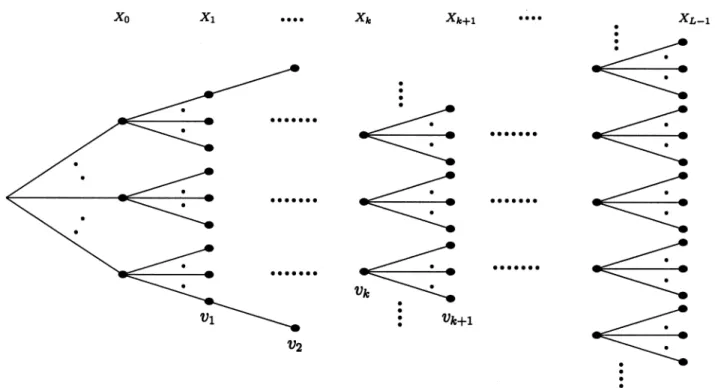
Fig. 1. Tree that represents all possible candidate sequences and the node values,fv ; k = 0; 1; . . .g, associated with nodes in the tree.
basic principle of branch-and-bound [16], and uses an uncon-strained solution obtained by using some inherent characteristic of the associated objective function. We also derive a recursive formula for the unconstrained minimum value, greatly reducing the complexity of our algorithm.
A. General Problem and Algorithm
Consider the general problem. Find the minimum value of a multivariate real-valued objective function
, where ,
being the cardinality of . We call a sequence a candidate sequence. A straightforward approach to obtain the solution is evaluating for all candidate sequences . Fig. 1 plots a tree related to this search problem. Every node in the tree has branches stemming from it, each connecting to a different descendent node. The descendent nodes of the root (i.e., the leftmost node of the tree) represent all possible values of taken from , and are called nodes of depth 0. In general, a node of depth has descendent nodes of depth , each denotes a possible value of , and the depth of the tree associated with the objective function is . A complete path in the tree is a path that starts at the root and ends at the tree tip. Each complete path contains nodes of depth 0 to and
represents a candidate sequence ,
where corresponds to the depth- node of this path.
Let be a partial path of length , and
define the node value of a node of depth associated with this partial path as
with known and fixed (18)
where denotes the set of complex numbers. Note that are “free” variables whose values are allowed to be any complex numbers without constraining them to be in . For every descendent node of the last node of , we compute the corresponding node value according to
with known and fixed (19)
Comparing (18) and (19), we see that as (18) has less constraint (or a larger degree of freedom). Hence, the node values of a path satisfy
(20) Equation (18) implies that the node value of a node at one of the tips of a tree is equal to where is the corresponding candidate sequence. The problem of finding the minimum value of is equivalent to finding the minimum node value amongst all tip nodes of the corresponding tree. As our tree structure implies that there is only one path from the root to a tip node, our problem becomes that of searching for the path whose last node has the minimum node value.
Before the search, we can assign a “reference solution” , which can be obtained either by the approximation solution of Section II-B or by other proper methods. In the process of searching for the “correct” path of a tree, if a node whose node value is larger than the reference metric , then (20) implies that for those candidate sequences ’s whose corre-sponding paths pass through this node, . Thus, there is no need to search the subtree stemming from this node. On the other hand, when we visit a node of depth at the
tip of the tree and find , where is the corre-sponding candidate sequence, then we replace by and use it as the new reference metric in subsequent visits. At the end of the search process, the surviving will be the de-sired solution. The above procedure avoids searching all paths and makes the complexity of finding the solution computation-ally feasible.
B. Branch-and-Bound Algorithm
For our blind detection problem, the associated multivariate objective function is given by (13)
(21) where is a function of . The initial “reference solution” , as just mentioned, can be obtained by the approximation method of Section II-B.
Now consider the calculation of the node value of a node of depth . When such a node is visited, the partial path has been determined. The definition of , (18), requires that we find that minimizes . Let
, , and
(22)
where is a matrix, an
matrix, and a matrix. Then
(23) where we have used the property [see (12)]. While is determined by , is allowed to be any complex vector of length , as there is no constraint on the associated data vector. Taking derivative with respect to , we see that the objective function (23) is minimized when
(24) and the corresponding minimum value is
(25) where the constant matrices and are given by
(26) (27) and and are identity matrices of the same dimensions as those of and , respectively. Note that when (24) is satis-fied, we have (28) and then (29) which is (25). C. A Recursive Formula
To reduce the calculation of node values, we develop a recur-sive relation between and , the node value of a node of depth and that of one of its immediate descendent nodes of depth . For convenience and preciseness, we add a superscript to each vector and matrix appearing in (22)–(27) to signify that these quantities are related to nodes of depth . From (25) and (27), we obtain
(30)
(31)
where , and
. Equation (24) reveals that the corresponding unconstrained sequence for is
(32) It can be shown (see Appendix) that
(33)
where , is the th element of
the matrix , and is derived from (32) via
(34) being the first row of . Compared with (25), (33) clearly reduces much of the complexity of computing .
D. Summary of the Algorithm
We summarize the proposed algorithm in the following. The constant parameters ’s and ’s are independent of the re-ceived vector. They can be predetermined and prestored before the blind detector is activated. We refer to this portion of the al-gorithm as the precalculation stage.
Precalculation:
1) Let the block length be and the regression polynomial
degree be . Compute and store ,
, , and .
2) For , compute and store , , and
according to (22), and and based on (26) and (27).
3) Determine and , . By definition,
is the first row of , and is the th entry of .
Tree search:
1) Determine an initial estimate by the approx-imation method of Section II-B, and compute
, where .
2) Starting at the root node, calculate the node values of all its immediate descendent nodes. Visit the immediate descen-dent node with the smallest node value.
3) When visiting a node, calculate the node values of all its immediate descendent nodes. Go visiting the immediate de-scendent node with the smallest node value, if this node value is smaller than . Otherwise, discard all these imme-diate descendent nodes and the corresponding subtrees (i.e., all their descendent nodes).
4) When all descendent nodes of a node are either visited or discarded, go back to the immediate ancestor node. Among the unvisited immediate descendent nodes of this ancestor node, visit the one with the smallest node value, if this node value is smaller than .
5) On visiting a node of depth at the tip, if , then replace by and by the corresponding se-quence. Go back to the immediate ancestor node and follow the procedure of step 4.
6) The search process ends with as the desired solution when there are no more unvisited nodes.
Several remarks on the above algorithm are in order. R1. The stack algorithm used in decoding convolutional
codes can also be used as an alternative search method, replacing the path metric by the node value.
R2. Our simulation shows that, on the average, the number of nodes visited by the stack algorithm is about the same as that visited by the proposed algorithm. How-ever, our algorithm does not have to perform stack sorting, and furthermore, for the stack algorithm, the number of stored nodes is unpredictable and may be-come very large at low SNRs, though the inequality (20) can be used to reduce the stack size. On the other hand, the number of stored nodes of the above algo-rithm is upper bounded by .
R3. The Fano metric has been proved to be optimal in additive white Gaussian noise (AWGN) channels in the sense it gives the best one-step prediction [14]. The stack algorithm, when using the Fano metric, usu-ally renders very fast searching speed. The node value, , plays a similar role to the Fano metric in AWGN, providing a (model-constrained) optimal one-step pre-dictor in a channel with memory.
R4. A good initial estimate (upper bound) is crucial for reducing the search time.
R5. For a convolutional-coded OFDM system, blind de-coding can be carried out in a similar manner with reduced complexity, by merging subtrees originating from the same state. But the corresponding code tree cannot be permuted, as suggested in Section IV-B, to accelerate the search speed.
IV. RELATEDDESIGNISSUES
We now address some related design issues and modifica-tions, some of which lead to much less complex algorithms for both blind and semiblind (low pilot density) detections.
A. Ambiguity Problem
When the estimated data sequence for the th subchannel is obtained, we still have to resolve the phase ambiguity associated with any blind equalizer for signals with symmetric constellation. For example, if is a solution of (13), and the square 16-quadrature amplitude mod-ulation (QAM) is used, then and are also solutions of (13). We can avoid the ambiguity issue by employing dif-ferential modulation, e.g., difdif-ferential -ary phase-shift keying (MPSK) or differential 16 STAR-QAM [13]. Coding (e.g., rota-tional-invariant trellis codes) is another alternative to eliminate the ambiguity. The simplest solution is obtained by using a few pilot symbols. As pilots are used only for resolving the phase ambiguity, they can be much sparser than those used in pilot-aided equalizers. Let the interpilot distance be symbols, where is the block length. If , blocks without pilots can derive the phase information from the preceding pilot-in-serted blocks.
Adjacent subchannels can also be used jointly to determine the phase rotation. Letting the estimated data sequence of the th subchannel be , we should choose such that best matches (4). More specifically, we select
such that
(35) where is one of the candidate ambiguity angles.
B. Influence of the Search Order and Its Implications
The sequence shown on top of Fig. 1 indicates a tree search in natural order, i.e., from to . Let
be a permutation of . The corresponding
rear-ranged sequence is now
associ-ated with a tree whose depth- nodes are relassoci-ated to the possible values of .
When performing the search process in this new tree, there is essentially no change of algorithmic complexity and logical procedure. We only have to replace by , where
is related to by
(36) and modify the corresponding parameters ’s and ’s accordingly. As our goal is to find a data sequence that minimizes (13), the order of finding the component values of the sequence is immaterial. Moreover, the final solution obtained by our algorithm is independent of the order of search. However, the search order does have some critical impacts.
Recall that the orthogonal projection in the objective function (21) is used to find the regression curve that fits the channel estimate in the LS sense (which is ). On the one hand, we are looking for a smooth curve to fit ; on the other hand, the components of tend to dictate and bound the “shape” of the candidate LS regression curve. If the final curve is smooth enough, the projection of the subsequence that consists of, say, two end points and the middle point alone,
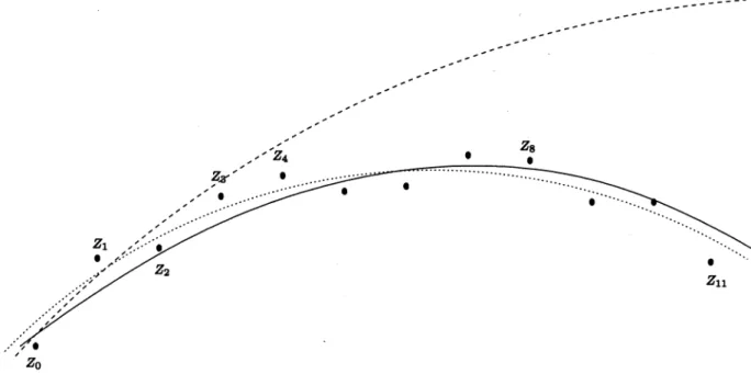
Fig. 2. Regression curve resulting from the natural search order(Z ; Z ; Z ; Z ) (the dash curve), and that due to a preferred uniformly contracting Z search order(Z ; Z ; Z ; Z ) (the dot curve). The actual values are indicated by the solid curve.
i.e., , where the integer
part of , will give a crude but probably acceptable approxi-mation. Using two additional middle points to form the new
subsequence ,
we obtain a better approximation by the projection . If, instead, we use the first three points or the first five points, for LS fitting, we are likely to obtain curves that are far from the final solution; see Fig. 2 for an example.
The above geometric property of LS-fitted solutions has two important implications:
1) the convergence speed of our tree-search algorithm, i.e., the number of nodes visited before the “distance” be-tween the corresponding LS-fitted curve and the final so-lution is within an acceptable bound, does depend on the order of our search;
2) in most cases, a good approximation of the final LS-fitted curve can be obtained by using only a few properly se-lected components of .
1) suggests that a preferred search order is the contracting
zigzag pattern , where the
integers denote the data locations. For example, if the sequence length 10, a preferred order is (0, 9, 5, 2, 7, 1, 3, 6, 4, 8). On the other hand, 2) indicates that we can reduce the search complexity by estimating the CRs based on the received samples at some selected locations to begin with, then use the estimated CRs for detecting data at the remaining locations. Often, we achieve significant complexity reduction with neg-ligible performance degradation by using the preferred search order and selective detection. For example, if , we
can use, say to estimate and
via the proposed tree-searching algorithm. Fig. 2 indicates that when this much-shortened search is
finished, already the implicit regression curve comes very close to the desired one. Given the CR estimates
derived from the curve, we then make hard decisions on , to determine the remaining ’s.
C. Partially Known Sequences and Semiblind Detection
In some situations, a few elements of the sequence in (13) are known or have been detected. These known symbols may be pilots, or mem-bers of the overlapped part of the current and the previous blocks. Denote the detected or known symbols in by . We can arrange the search order so that it begins with these known symbols, followed by the
undetected symbols . Since the first
symbols are known, the tree degenerates to one with only one branch for the beginning nodes.
Semiblind schemes refer to those that use sparse pilot sym-bols. Besides resolving the phase ambiguity, these few pilot symbols can, as mentioned before, be used to reduce the tree size and provide an initial reference solution and reference metric. We can apply any conventional pilot-assisted method to obtain the reference sequence and metric.
Let us consider a semiblind scheme where two pilots are lo-cated at both ends of a block. We apply the blind algorithm with the preferred search order that starts at the pilot positions 0 and . An initial reference solution is obtained by using the two pilots only. To detect the remaining data, we conduct the tree search to level , where we can choose to reduce the complexity. This scheme will be referred to as the low-complexity semiblind (LCSB) detector.
Note that the pilot-assisted scheme proposed in [5] corsponds to the case when the search order is such that the re-sulting tree is partially degenerated with the search depth equal to the number of pilots.
Fig. 3. BEP performance of the differential QPSK-OFDM system with or without blind channel estimation.
V. NUMERICALRESULTS ANDDISCUSSIONS
Numerical results reported in this section assume an OFDM system that has a total bandwidth of 1 MHz, 32 equally spaced mutual-orthogonal subchannels, and a symbol time (included guard interval) of 34.5 s. A four-ray Jakes’ model [15] is used to simulate a time-varying Rayleigh fading channel with relative power strengths 0.5938, 0.7305, 0.3175, 0.1137, and delays 0, 0.1, 0.5, 1 s, respectively. As mentioned before, the algorithms presented in the previous two sections are 1-D solutions. Except for Section V-C, we assume that a 1-D algorithm is carried out on each subchannel for detecting OFDM signals.
A. Differential Encoding Schemes
The first case we consider is the differential scheme that employs a quaternary phase-shift keying (QPSK) or 16 STAR-QAM [13] signal. The (time) block length used is symbols. Figs. 3 and 4 plot the bit-error probability (BEP) performance curves of differential QPSK (DQPSK) and 16 STAR-QAM systems using the algorithm presented in Section III-D. The performance of the uncompensated systems, i.e., those labeled by “without BE” (blind equalization), is also given in those two figures. It can be seen that the proposed blind detection scheme does enhance the performance of both systems and yields no obvious error floor.
B. Semiblind Scheme (I)
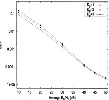
For the semiblind scheme, very few pilots are available, and they are used only for eliminating the phase ambiguity and pro-viding the initial channel estimation. In each subchannel, we insert one pilot symbol for every blocks with a block length of , or equivalently, every symbols. The pilot density is much sparser than that of the conventional pilot-as-sisted schemes for time-varying channels [5]. Fig. 5 plots the BEP performance for the square 16QAM-OFDM system with and normalized Doppler shift 0.00414. We notice a small increase in BEP occurs when increases, especially
Fig. 4. BEP performance of the differential 16 STAR-QAM-OFDM system with or without blind channel estimation.
Fig. 5. BEPs of the 16QAM-OFDM system using the semiblind detector with full searching depth;f T = :004 14.
at high SNRs. There are no clear error floors within the range of interest, though.
C. Semiblind Scheme (II) (Low-Complexity Scheme)
The performance of the LCSB algorithm described in Sec-tion IV-C is given in Fig. 6, with and search depth ( yields almost identical performance). The two pilot symbols within a block are at positions 0 and 20, re-spectively. We adopt the contracting- search pattern that be-gins with the pilot positions 0 and 20. For , the search order is 0, 20, 10, and then 5. The normalized Doppler shift is , which corresponds to a fast time-varying channel. We also plot the BEP curves of the ideal receiver that has perfect channel estimate and the conventional pilot-assisted scheme. The performance of the ideal receiver provides the absolute
Fig. 6. BEPs of the 16QAM-OFDM system using the LCSB detector with a single pilot at both ends of a block;f T = 0:01. The search depth is L = 3 for both degree 1 and 2 models.
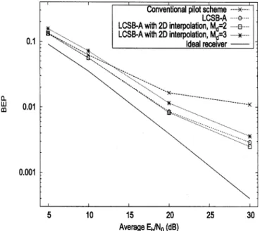
Fig. 7. BEPs of the 16QAM-OFDM system using the LCSB two-stage algorithm with a 2-D regression model. The system and channel parameters are the same as Fig. 6. The curve labeled by LCSB-A is the same as the the curve labeled by “Low complexity semiblind, deg= 1” in Fig. 6.
lower bound for comparison. Since the channel is fast fading and there are only two pilots in a block, the pilot-assisted scheme cannot give a reliable channel estimate.
The LCSB estimate has more impressive relative perfor-mance gain at high SNRs. For SNR less than 10 dB, however, using a degree-2 polynomial model may degrade the perfor-mance, though it greatly improves the performance at SNR higher than 30 dB. In most cases, the performance is only a few decibels away from that of the ideal receiver. Such a behavior has been expected, as a higher order model involves more parameters, and the channel estimation error which dictates
Fig. 8. BEPs of the 16QAM-OFDM system using the LCSB two-stage algorithm with a 2-D regression model. The system and channel parameters are the same as Fig. 6. The curve labeled by LCSB-B is the same as the the curve labeled by “Low complexity semiblind, deg= 2” in Fig. 6.
the BEP performance is mainly caused by thermal noise at low SNRs, while the modeling error dominates at high SNRs.
The performance of the two-stage algorithm described in Sec-tion II-A is plotted in Fig. 7. The semiblind algorithm is em-ployed on every subchannels, then the detected symbols are treated as pilots, so that the 2-D model-based algorithm of [5] can be used to detect the remaining symbols.
For comparison, Fig. 7 presents the performance of the detector that uses the LCSB scheme with degree-1 polynomial model (labeled by LCSB-A) on all subchannels under the same system and channel conditions. As the 2-D model takes into account the correlations among subchannels, the two-stage scheme outperforms LCSB-A for the case . For , the correlation between two detected subchannels be-comes less obvious, and the resulting modeling error degrades the performance of the two-stage algorithm. Fig. 8 provides a similar comparison for the LCSB scheme with a degree-2 polynomial model (labeled by LCSB-B). Similar to the 1-D case shown in Fig. 8, a higher degree model yields smaller modeling error, and thus better BEP performance at high SNRs.
D. Complexity
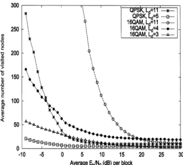
Fig. 9 shows the average number of visited nodes for de-tecting QPSK and 16QAM signals with different search depths ( ). The average or SNR per block in this figure de-notes the “locally” average SNR within a block of OFDM sym-bols as our algorithms operate in a block-by-block fashion. Note that even if the average is 10 dB, the received signal may suffer from severe fading in a few consecutive blocks, where the average per block is far less than 0 dB. It is more appro-priate to present the complexity performance in terms of average
per block.
We see that for larger average SNRs, the visited number is very small for all cases, while if the average SNR is smaller than a threshold, which depends on the signal constellation size
Fig. 9. Average number of visited nodes within a block for detecting QPSK-OFDM and 16QAM-OFDM signals with different search depthsL .
Fig. 10. Average number of real multiplications per symbol in the tree-search process for the LCSB scheme withL = 21.
and the search depth, the visited node numbers increase rapidly. On the other hand, adopting the partial search algorithm (
) greatly reduces the number of visited nodes, especially at low SNRs. The curves and (with the search order 0, 20, 10, 5, and 15) correspond to the LCSB schemes of Fig. 6. We also show in Fig. 10 the average number of real multiplications per symbol in a block of length , which corresponds to the curves and in Fig. 9. We see that for the case , we need about 30 real multiplications for each symbol per subchannel when the average SNR within a block is 9 dB.
Using the complete blind algorithm of Section III-D for every subchannel is expected to require high computing complexity at low and medium SNRs. Therefore, we have proposed var-ious reduced-complexity derivative algorithms, and have just shown that, if a preferred search order together with a reduced
search-depth scheme are used, the resulting complexity is only moderate. The availability of few pilots (semiblind) helps in re-ducing the complexity. The numbers in the above two figures are obtained on a per-subchannel basis, hence, the two-stage al-gorithm will bring further complexity reduction. However, the complexity of our algorithms is lower bounded by that of [5], as both use the same model-based approach.
VI. CONCLUSION
In this paper, we present new joint detection and estimation methods for blindly and semiblindly detecting OFDM signals in a fading environment, where the CR may vary from symbol to symbol. Based on a regression model, we formulate the blind detection problem as an integer programming problem. We then apply an elementary inequality and the branch-and-bound prin-ciple to find the optimal solution. A recursive formula is derived to simplify the computation effort. We propose low-complexity variations that use the concepts of preferred search order and se-lective detection. A two-stage algorithm is suggested to reduce the overall detection complexity, and numerical examples are given to examine the performance and complexity of the pro-posed blind and semiblind detection schemes. Our algorithms are shown to be effective in combating fast channel variations and in providing satisfactory system performance.
APPENDIX
DERIVATION OF ARECURSIVEFORMULA Let and be the node values of a node of depth and one of its immediate descendent nodes of depth , respec-tively. From (25) and (27), we have
(A.1)
(A.2)
where , and
. The corresponding unconstrained sequence for is (A.3) Let Since (A.4) and
we obtain
(A.5) Invoking (24) and (26), we obtain
(A.6) i.e., the elements in the lower part of the vector in the left-hand side of (A.5), from the th to the th elements, are all zero. Hence, the corresponding elements in the right-hand side of (A.5) are also zero, and we have
(A.7) (A.8) where denotes the th elements of the vector . Multi-plying the right-hand side of (A.5) by and using (A.8), we obtain
(A.9) Comparing (A.9) with (A.2) and noticing that
, where , we obtain
(A.10) Substituting (A.7) and (A.8) into (A.10) and invoking (27), we obtain the desired recursive formula
(A.11)
where is the th element of .
ACKNOWLEDGMENT
The authors wish to thank the the anonymous reviewers and the Associate Editor, G. M. Vitetta, for their comments and sug-gestions that helped improve the presentation of the paper.
REFERENCES
[1] O. Edfors et al., “OFDM channel estimation by sigular value decompo-sition,” IEEE Trans. Commun., vol. 46, pp. 931–939, July 1998. [2] Y. (G.) Li et al., “Robust channel estimation for OFDM systems with
rapid diversity fading channels,” IEEE Trans. Commun., vol. 46, pp. 902–915, July 1998.
[3] V. Mignone and A. Morello, “CD3-OFDM: A novel demodulation scheme for fixed and mobile receivers,” IEEE Trans. Commun., vol. 44, pp. 1144–1151, Sept. 1996.
[4] M.-X. Chang and Y. T. Su, “2-D regression channel estimation for equal-izing OFDM signals,” in Proc. IEEE 51st Vehicular Technology Conf., Tokyo, Japan, May 2000, pp. 240–244.
[5] , “Model-based channel estimation for equalizing OFDM signals,”
IEEE Trans. Commun., vol. 50, pp. 540–544, Apr. 2002.
[6] R. W. Heath and G. B. Giannakis, “Exploiting input cyclostationarity for blind channel identification in OFDM systems,” IEEE Trans. Signal
Processing, vol. 47, pp. 848–856, Mar. 1999.
[7] H. Bölcskei, P. Duhammel, and R. Hleiss, “A subspace-based approach to blind channel in pulse shaping OFDM/OQAM systems,” IEEE Trans.
Signal Processing, vol. 49, pp. 1594–1598, July 2001.
[8] Y. Song, S. Roy, and L. A. Akers, “Joint blind estimation of channel and data symbols in OFDM,” in Proc. Vehicular Technology Conf., vol. 1, Tokyo, Japan, 2000, pp. 240–244.
[9] S. Zhou and G. B. Giannakis, “Finite-alphabet based channel estimation for OFDM and related multicarrier systems,” IEEE Trans. Commun., vol. 49, pp. 1402–1414, Aug. 2001.
[10] M. Luise, R. Reggiannini, and G. M. Vitetta, “Blind equalization/dec-tection for OFDM signals over frequency-selective channels,” IEEE J.
Select. Areas Commun., vol. 16, pp. 1568–1578, Oct. 1998.
[11] M.-X. Chang and Y. T. Su, “Blind joint channel and data estimation for OFDM signals in Rayleigh fading,” in Proc. IEEE 53st Vehicular
Technology Conf., Rhodes, Greece, May 2001, pp. 791–795.
[12] R. Raheli, A. Polydoros, and C.-K. Tzou, “Per-survivor processing: A general approach to MLSE in uncertain environments,” IEEE Trans.
Commun., vol. 43, pp. 354–364, Feb.-Apr. 1995.
[13] T. T. Tjung et al., “On diversity reception of narrowband 16 STAR-QAM in fast Rician fading,” IEEE Trans. Veh. Technol., vol. 46, pp. 923–932, Nov. 1997.
[14] J. Massey, “Variable-length codes and the Fano metric,” IEEE Trans.
Inform. Theory, vol. IT-18, pp. 196–198, Jan. 1972.
[15] W. C. Jakes, Microwave Mobile Communications. New York: Wiley, 1974.
[16] H. A. Taha, Integer Programming, Theory, Applications, and
Computa-tions. New York: Academic, 1975.
Ming-Xian Chang (M’02) received the B.S. degree
in electrical engineering from National Taiwan University, Taipei, Taiwan, R.O.C., in 1995, and the M.S. and Ph.D. degrees in communication engineering from National Chiao Tung University, Hsinchu, Taiwan, R.O.C., in 1997 and 2002, respectively.
Since August 2002, he has been with National Cheng Kung University, Tainan, Taiwan, R.O.C., where he is currently an Assistant Professor in the Department of Electrical Engineering. His research interests include wireless communication systems and signal processing.
Yu T. Su (S’81–M’82) received the Ph.D. degree
from the University of Southern California, Los Angeles, in 1983.
From 1983 to 1989, he was with LinCom Corporation, Los Angeles, CA, where he was a corporate scientist, involved in the design of various measurement and digital satellite communication systems. Since September 1989, he has been with National Chiao Tung University, Hsinchu, Taiwan, R.O.C., where he was Head of the Communication Engineering Department between 2001 and 2003. He is also affiliated with the Microelectronics and Information Systems Research Center of the same university, and served as a Deputy Director from 1997 to 2000. His main research interests include communication theory and statistical signal processing.