在以道路基礎蜂巢式網路中以馬可夫決策為基礎並使用鄰近狀態資訊的允入控制機制

全文

(1)國立交通大學電信工程學系碩士班碩. 士. 論. 文. 在以道路基礎蜂巢式網路中以馬可夫決策為基礎並使用鄰近狀態資訊的允入控制機制. Markov-Decision-Based Call Admission Control with State Information of Adjacent Cells in Road-based Cellular Networks. 研究生：曹賢宗. Student: Hsien-Tsung Tsao. 指導教授：廖維國博士. Advisor: Dr. Wei-Kuo Liao. 中華民國九十七年五月.

(2) 在以道路基礎蜂巢式網路中以馬可夫決策為基礎並使用鄰近狀態資訊的允入控制機制 Markov-Decision-Based Call Admission Control with State Information of Adjacent Cells in Road-based Cellular Networks. 研究生：曹賢宗. Student: Hsien-Tsung Tsao. 指導教授：廖維國博士. Advisor: Dr. Wei-Kuo Liao. 國立交通大學電信工程學系碩士班碩士論文 A Thesis Submitted to the Department of Communication Engineering College of Electrical and Computer Engineering National Chiao Tung University in Partial Fulfillment of the Requirements for the Degree of Master of Science In Communication Engineering May 2008 Hsinchu, Taiwan, Republic of China.

(3) 在以道路基礎蜂巢式網路中以馬可夫決策為基礎並使用鄰近狀態資訊的允入控制機制研究生：曹賢宗. 指導教授：廖維國博士. 國立交通大學電信工程學系碩士班. 中文摘要在此篇論文中，我們研究將以固定通道(Fix Channel Allocation)分配蜂巢式網路鄰近狀態資訊列入考慮的允入控制機制。在某種程度的假設前提之下，對於每個細胞，我們使用二維狀態的馬可夫鏈(Markov chain)來模擬此系統。其第一維是代表基礎細胞的 50 個狀態，其第二維是代表周圍細胞的 300 個狀態。因此，我們的模型變成一個總共 15000 狀態數的二維馬可夫鏈。對於以最小化新連線的阻斷率(new call blocking probability)和連線交遞的失敗率(handoff dropping probability)為目標函數的問題，可用馬可夫決策過程 (Markov Decision Process)來描述。然而，此一龐大的狀態數目使得轉置機率的反矩陣(其大小為 2.25×108)無法計算出來，也因此複雜化了應用馬可夫決策過程中的「策略疊代法」 (policy-iteration method)來解決我們的問題。於是我們使用把在幾步之內可以到達的狀態們群集在一起的「狀態聚合法」(state aggregation method)來克服此困難。如此做了之後，我們的模型變成總共只有 66 個狀態而且可用「策略疊代法」來解。最後，我們證實與熟知的「保護頻道策略」(Guard Channel policy)相比較之下，我們的策略可以很容易的得到並且有較低的平均成本。然而，以通道借償並隨方向鎖定(Borrowing with Directional Locking)的通道分配方式比固定通道分配方式能有更好的通話失敗率。因此我們多加入單步決策(One-Step Policy)來改變以上碼可夫決策過程以期待得到更好的效能。. 中華民國九十七年五月. i.

(4) Markov-Decision-Based Call Admission Control with State Information of Adjacent Cells in Road-based Cellular Networks Student: Hsien-Tsung Tsao. Advisor: Dr. Wei-Kuo Liao. Department of Communication Engineering National Chiao Tung University. Abstract We study the admission control problem in cellular network when taking the neighboring state information into consideration with FA Strategy. For each cell, under certain assumptions, we model the system by Markov chain with two-dimensional states where the first dimension represents the base cell’s 50 states and the second dimension stands for the adjacent cells’ 300 states. As a result, the model becomes a two-dimensional Markov chain with 15000 states in total. The problem of minimizing a linear objective function of new call blocking and handoff call dropping probabilities can then be formulated as a Markov Decision Process. However, the enormous number of states makes the inverse of the transition probability matrix (which is of size 2.25×108) computation-prohibitive and thus complicates the application of policy iteration method in the context of Markov Decision Process to solve our problem. To attack such, we use the state aggregation method where we group those states which basically are few steps reachable from each other. After doing so, our model turns into involving only 66 states in total and solvable by the policy-iteration method. Finally, we show that our policy can be easily derived and has lower average cost than the well-known Guard Channel policy. However, we find that BDCL strategy outperforms FA strategy. Therefore, we modify the above MDP model by adding One-Step policy to it in order to get better efficiency.. ii.

(5) 致謝首先誠摯的感謝指導教授廖維國博士，老師悉心的教導使我得以一窺領域的深奧，不時的討論並指點我正確的方向，使我在這些年中獲益匪淺。老師對學問的嚴謹更是我輩學習的典範。本論文的完成另外亦得感謝的先生大力協助。因為有你的體諒及幫忙，使得本論文能夠更完整而嚴謹。兩年裡的日子，實驗室裡共同的生活點滴，學術上的討論、言不及義的閒扯、讓人又愛又怕的宵夜、趕作業的革命情感、因為睡太晚而遮遮掩掩閃進實驗室........，感謝眾位學長姐、同學、學弟妹的共同砥礪(墮落?)，你/妳們的陪伴讓兩年的研究生活變得絢麗多彩。感謝廖怡翔學長、林國瑋學姐們不厭其煩的指出我研究中的缺失，且總能在我迷惘時為我解惑，也感謝陳憲良、黃健智、林于彰同學的幫忙，恭喜我們順利走過這五年。實驗室的陳俊宏、柯富元、游永裕學弟、陳郁媛、林柔嫚學妹們當然也不能忘記，妳的幫忙及搞笑我銘感在心。女朋友在背後的默默支持更是我前進的動力，沒有的體諒、包容，相信這兩年的生活將是很不一樣的光景。而好友 Chrislove 不計名份的陪伴更是令人感動，在此一併致謝。最後，謹以此文獻給我摯愛的雙親。. iii.

(6) Contents Chinese Abstract ......................................................................................................................... i English Abstract ......................................................................................................................... ii Acknowledgement ..................................................................................................................... iii Contents ..................................................................................................................................... iv List of Figures ............................................................................................................................ vi List of Tables............................................................................................................................. vii Chapter 1. Introduction ....................................................................................................... - 1 -. Chapter 2 Background Knowledge .................................................................................... - 3 2.1 Minimizing a Linear Objective Function (MINOBJ) ............................................... - 3 2.2 Guard Channel Policy ................................................................................................. - 3 2.3 Markov Decision Process ............................................................................................ - 4 2.3.1 State ........................................................................................................................ - 4 2.3.2 Transition Probability ........................................................................................... - 5 2.3.3 Rewards ................................................................................................................. - 5 2.3.4 Expected Immediate Reward ............................................................................... - 6 2.3.5 Alternatives ............................................................................................................ - 6 2.3.6 Policy ...................................................................................................................... - 7 2.3.7 Gain ........................................................................................................................ - 7 2.4 The Policy-Iteration Method ....................................................................................... - 8 2.4.1 The Iteration Cycle ............................................................................................... - 8 2.5 The State Aggregation Method ................................................................................. - 10 2.6 BDCL(Borrowing with Directional Channel Locking) .......................................... - 11 Chapter 3 System Specification ........................................................................................ - 14 3.1 Base Station ................................................................................................................ - 14 3.2 Mobile Station ............................................................................................................ - 15 3.3 Channel ....................................................................................................................... - 15 Chapter 4 Problem Formulation by MDP in FA Strategy ............................................. - 17 And Proposed Method ......................................................................................................... - 17 4.1 Our Model................................................................................................................... - 17 4.2 Alternatives and Costs ............................................................................................... - 18 4.3 Our Policy-Iteration Method .................................................................................... - 19 4.4 Our State Aggregation Method ................................................................................ - 21 iv.

(7) Chapter 5 Modification from FA to BDCL by One-Step Policy And Update Rules of Policy with Time-varying MDP Parameters ...................................................................... - 23 5.1 Effects of Borrowing Operation ............................................................................... - 23 5.2 One-Step Policy for BDCL Strategy ......................................................................... - 26 5.3 Update Rules of Policy with Time-varying MDP Parameters ............................... - 27 Chapter 6 Simulator and Results ..................................................................................... - 30 6.1 Simulator Settings ...................................................................................................... - 30 6.2 UML Statechart of Our Model.................................................................................. - 32 6.3 Simulation Results ..................................................................................................... - 36 Chapter 7 Conclusion ........................................................................................................ - 48 References ............................................................................................................................. - 49 -. v.

(8) List of Figures Fig 2.1 Guard Channel policy ............................................................................................... - 4 Fig. 2.2 Diagram of states and alternatives.1....................................................................... - 7 Fig. 2.3 The iteration cycle.2 ................................................................................................. - 9 Fig. 2.4 An example of aggregate Markov chain. .............................................................. - 11 Fig 2.5 an example of regular cells ..................................................................................... - 12 Fig. 3.1 Fully connected network architecture. ................................................................. - 14 Fig. 3.2 Total states diagram of the two-dimensional Markov chain. ............................. - 16 Fig. 4.1 State transition diagram ........................................................................................ - 18 Fig. 4.2 Transition diagram with alternatives 1 and 2.6 ................................................... - 19 Fig. 4.3 Make two-dimensional Markov chain into smaller groups ................................ - 22 Fig 5.1 Transition diagram of 3 alternatives when new call, handoff call arrive for Base Cell......................................................................................................................................... - 23 Fig 5.2 Transition diagram for alternatives 1, 2 and 3 ..................................................... - 24 Fig 5.3 Effect of borrowing operation on adjacent cells ................................................... - 25 Fig 5.4 Example of effect by borrowing operation on adjacent cells .............................. - 25 Fig 5.5 Example of effect by borrowing operation on adjacent cells .............................. - 26 Fig 5.6 One-Step Policy ........................................................................................................ - 27 Fig 6.1 Road Topology Example for Simulation ............................................................... - 31 Fig 6.2 OMD of the Simulator ............................................................................................ - 32 Fig 6.3 State Chart of Mobile .............................................................................................. - 33 Fig 6.4 State Chart of Map .................................................................................................. - 34 Fig 6.5 State Chart of Cell ................................................................................................... - 34 Fig 6.6 Call Block Rate of different method under different loads ................................. - 36 Fig 6.7 Call Drop Rate of different method under different loads .................................. - 37 Fig 6.8 Call Failure Rate of different method under different loads............................... - 38 Fig 6.9 Map of road topology in Cell 16, Cell 57 and Cell 62........................................... - 39 Fig 6.10 Parameters update for load 70 Cost 5-30 of period 15 sec ................................ - 39 -. vi.

(9) Fig 6.11 Parameters update for load 70 Cost 5-30 of period 60 sec................................. - 40 Fig 6.12 Parameters update for load 70 Cost 5-30 of period 120 sec .............................. - 40 Fig 6.13 Parameters update for load 70 Cost 5-30 of period 180 sec .............................. - 41 Fig 6.14 Parameters update for load 70 Cost 5-30 of period 240 sec .............................. - 41 Fig 6.15 Parameters update for load 70 Cost 5-30 of period 300 sec .............................. - 42 Fig 6.16 Parameters for load 70 Cost 5-30 without periodic update ............................... - 42 Fig 6.17 Average cost of Load 70 Cost 5-30 with different update periods .................... - 43 Fig 6.18 Average cost of Load 90 Cost 5-30 with different update periods .................... - 44 Fig 6.19 Average cost of Load 100 Cost 5-30 with different update periods .................. - 44 Fig 6.20 Average cost of Load 150 Cost 5-40 with different update periods .................. - 45 Fig 6.21 Average cost of Load 150 Cost 5-45 with different update periods .................. - 45 Fig 6.22 Average cost of Load 200 Cost 5-50 with different update period .................... - 46 Fig 6.23 Average cost of Load 200 Cost 5-60 with different update period .................... - 46 -. List of Tables Table 5.1 Alternatives of One-Step Policy .......................................................................... - 27 Table 5.2 Parameters update rules ..................................................................................... - 28 Table 6.1 Aggregation of total states ................................................................................... - 35 Table 6.2 Alternatives of base cell’s states. ........................................................................ - 36 -. vii.

(10) Chapter 1 Introduction. In the cellular system, the entire spectrum is divided into a number of channels. In the channel assignment scheme [1], channels then are assigned to a cell, in either static or dynamic way, in principle of that adjacent cells cannot share (or reuse) the same channel to reduce the co-channel interference. As a result, when a mobile with a call in progress moves from the original cell into an adjacent cell, the base stations must perform the handoff operation, i.e., the currently-used channel in the original cell should be returned to the cell and the adjacent cell attempts to find a new channel for the mobile. Though the cellular system in this way boosts the wireless spectrum, yet the cell may still drop a handoff call or simply block a new call because available channels in the cell are insufficient in FA (Fixed-channel Allocation) scheme. To handle such a limited spectrum problem, the Guard Channel policy [2] determines the number of channels reserved for handoff calls by only considering the status of the local cell. With certain assumptions, such as constant arrival rate of handoff calls, the problem of minimizing a linear objective function (MINOBJ) of new call blocking and handoff call dropping probabilities can be formulated and solved by using Markov Decision Process (MDP) models. It is worthwhile to stress that the Guard Channel policy is obtained without considering neighboring cells’ information. In [3], the author found that it is worthwhile to explore the neighboring cell’s information. To this end, they proposed a predictive and adaptive scheme for bandwidth reservation for handoff calls. By using the ongoing call’s mobility history of neighboring cells to formulate the handoff estimation function, the handoff dropping probability can be kept below a target value. We can see from the simulation result that although the computation complexity of its best scheme is 1.5 times higher than using local cells’ information only, it works well under a variety of traffic loads, connection bandwidths, and mobility. Still it isn’t the optimal scheme since there is a better scheme in the simulation result for the time-varying case. In this thesis, we consider using MDP model to find the optimal admission control in the -1-.

(11) presence of the neighboring cells’ information. Since the neighboring cells’ ongoing calls are encoded in the states of our model, this becomes a two-dimensional MDP problem. We solve this problem by the policy-iteration method which includes Gaussian elimination method to find the inverse matrix of the transition probability matrix. Since the state-space of two-dimensional MDP extends from n to 6n2. The computation complexity of the inverse matrix is then increased from 6n2 to 36n4, which is impracticably large. In order to conquer this, we use the state aggregation method which groups several states together into a big state to reduce the size of the inverse matrix. Finally, as the simulation results shown, our method is not only viable but also has average cost lower than Guard Channel policy. We find that BDCL (Borrowing with Directional Channel Locking) channel allocation strategy outperforms FA in call failure rate, and therefore, we may propose BDCL instead of FA to make the efficiency better. However, with BDCL strategy we have to know information of all adjacent cells but just that of neighboring cells. In this aspect, we may just modify the above MDP model to fit BDCL strategy, because the main difference between FA and BDCL scheme is “Borrowing” operation from the neighboring cell. We will just add One-Step-Policy to facilitate the computational result, which includes the policies and values, of the original MDP model. However, the parameters, like arrival rate, handoff rate, departure rate, in the MDP model varies with time, therefore, we have to adjust the parameters periodically to fit the actually ones. For the above purpose, we will measure difference between the system cost that is due to rejecting calls and the model cost that is derived from the gain of MDP computational result. After getting the difference, we will have our update rule in order to predict the parameters of the next duration. Furthermore, our simulation will run under the road topology environment, it would be more realistic and closer to the real system. The rest of the thesis is organized as follows. In chapter 2, we introduce the background knowledge of our study. The system specification is presented in chapter 3. The formulation of our problem by MDP and the proposed method is described in chapter 4. Modification from FA to BDCL by One-Step Policy and update rules of policy with time-varying MDP parameters are described in chapter 5. Our simulator design and simulation results are illustrated in chapter 6. In chapter 7, we make conclusion.. -2-.

(12) Chapter 2 Background Knowledge. In this chapter, we will introduce the basic idea of MINOBJ, Guard Channel policy [4], Markov Decision Process with rewards, the policy-iteration method [5], the state aggregation method [6] and BDCL(Borrowing with Directional Channel Locking) channel allocation scheme [22]. In MDP, we will give formal definition to state, transition probability, expected immediate rewards, alternatives, policy and gain.. 2.1 Minimizing a Linear Objective Function (MINOBJ) Consider any policy π that determines the acceptance or rejection of new and handoff calls. Let constants A1 and A2 denote the penalties associated with rejecting new and handoff calls respectively. Note that we are only interested in values of A1 and A2 such that 0 < A1 < A2 since we would like to give handoff calls higher priority than new calls. Let π1n (π2n) be 0 or 1 depending on whether the nth new (handoff) call is accepted or rejected respectively. Then, we define N −1 1 ⎛ N −1 ⎞ φπ = lim E ⎜ ∑ A1π 1n + ∑ A2π 2 n ⎟ . N →∞ N n =0 ⎝ n =0 ⎠. (2.1). We are interested in determining optimal policy π* over the set of all call admission control policies π, i.e., find policy π* such that φπ * = min φπ . We note that Eq. (2.1) is a π. formulation for the average cost problem [7] with the cost of rejecting a handoff call being A2 and the corresponding cost for new call rejection being A1.. 2.2 Guard Channel Policy The notion of guard channels was introduced in the mid-80s, as a call admission mechanism to give priority to handoff calls over new calls [8]. In this policy, a set of channels -3-.

(13) called the guard channels are permanently reserved for handoff calls. In [9], Miller obtains a result which can be used to easily show that the Guard Channel policy is optimal for the MINOBJ problem. Consider a cellular network with C channels in a given cell. The Guard Channel policy reserves a subset of these channels (say C − T) for handoff calls. Whenever the channel occupancy exceeds a certain threshold T, the Guard Channel policy rejects new calls until the channel occupancy goes below the threshold. Note that this policy accepts handoff calls as long as channels are available, and is illustrated algorithmically in Fig. 2.1.. Fig 2.1 Guard Channel policy. 2.3 Markov Decision Process 2.3.1 State A Markov Process is a mathematical model that is useful in the study of complex systems. The basic concepts of the Markov process are those of “state” of a system and state “transition”. We say that a system occupies a state when it is completely described by the values of variables that define the state. A system makes state transitions when its describing variables change from the values specified for one state to those specified for another.. -4-.

(14) 2.3.2 Transition Probability Suppose that there are N states in the system numbered from 1 to N, then the probability of a transition from state i to state j during the next time interval, is a function only of i and j and not of any history of the system before its arrival in i. In other words, we may specify a set of conditional probabilities pij that a system which now occupies state i will occupy state j after its next transition. The transition probability matrix P is thus a complete description of the Markov process. 2.3.3 Rewards Suppose that an N-state Markov process earns rij dollars when it makes a transition form state i to state j. We call rij the “reward” associated with the transition from i to j. The set of rewards for the process may be described by a reward matrix R with elements rij. The Markov process now generates a sequence of rewards as it makes transitions from state to state. The reward is thus a random variable with a probability distribution governed by the probabilistic relations of the Markov process. One question we might ask concerning is: What will be the player’s expected winning in the next n transitions if the process is now in state i? To answer this question, let us define vi(n) as the expected total earnings in the next n transitions if the system is now in state i. Some reflection on this definition allows us to write the recurrence relation N. vi (n) = ∑ pij [rij + v j (n − 1)] j =1. i = 1, 2, L , N. n = 1, 2, 3, L.. (2.2). If the system makes a transition from i to j, it will earn the reward rij plus the amount it expects to earn if it starts in state j with one move fewer remaining. As shown in Eq. (2.2), these rewards from a transition to j must be weighted by the probability of such a transition, pij, to obtain the total expected rewards. Notice that Eq. (2.2) may be written in the form. -5-.

(15) N. N. j =1. j =1. vi (n) = ∑ pij rij + ∑ pij v j (n − 1). i = 1, 2, L , N. n = 1, 2, 3, L. (2.3). so that if a quantity qi is defined by N. qi = ∑ pij rij j =1. i = 1, 2, L , N .. Eq. (2.2) takes the form N. vi (n) = qi + ∑ Pij v j (n − 1) j =1. i = 1, 2, L , N. n = 1, 2, 3, L.. (2.4). 2.3.4 Expected Immediate Reward The quantity qi may be interpreted as the reward to be expected in the next transition out of state i; it will be called the “expected immediate reward” for state i. Rewriting Eq. (2.2) as Eq. (2.4) shows us that it is not necessary to specify both a P matrix and an R matrix in order to determine the expected earnings of the system. All that is needed is a P matrix and a q column vector with N components qi. The reduction in data storage is significant when large problems are to be solved on a digital computer. In vector form, Eq. (2.4) may be written as. v (n) = q + Pv(n − 1). n = 1, 2, 3, L. (2.5). where v(n) is a column vector with N components vi(n), called the total-value vector. 2.3.5 Alternatives The concept of “alternative” for an N-state system is presented graphically in Fig. 2.2. In this diagram, two alternatives have been allowed in the first-state. If we pick alternative 1 (k = 1 1), then the transition from state 1 to state 1 will be governed by the probability p11 , the 1 1 , from 1 to 3 by p13 , and so on. The transition from state 1 to state 2 will be governed by p12. rewards associated with these transitions are r111 , r121 , r131 , and so on. If the second alternative in -6-.

(16) state 1 is chosen (k = 2), then p112 , p122 , p132 , L, p12N and r112 , r122 , r132 , L, r12N , and so on, would be the pertinent probabilities and rewards, respectively. In Fig. 2.2, we see that if alternative 1 in state 1 is selected, we make transitions according to the solid lines; if alternative 2 is chosen, transitions are made according to the dashed lines. The number of alternatives in any state must be finite, but the number of alternatives in each state may be different from the numbers in other states.. Fig. 2.2 Diagram of states and alternatives. 2.3.6 Policy We shall define di(n) as the number of the alternative in the ith state that will be used at stage n. We call di(n) the “decision” in state i at the nth stage. When di(n) has been specified for all i and all n, a “policy” has been determined. The optimal policy is the one that maximizes total expected return (or minimizes total expected cost) for each i and n. 2.3.7 Gain -7-.

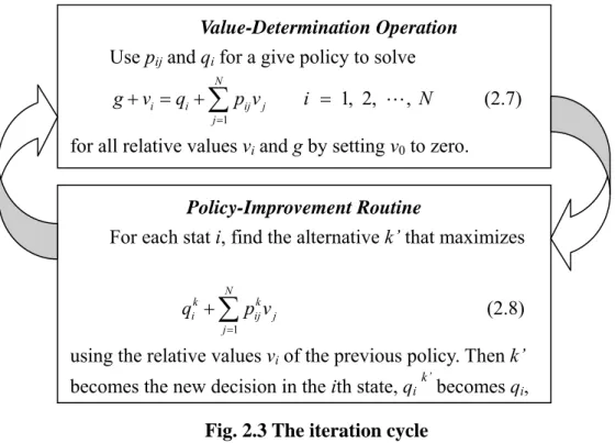
(17) Consider a completely ergodic N-state Markov process described by a transition probability matrix P and a reward matrix R. Suppose that the process is allowed to make transitions for a very, very long time and that we are interested in the earnings of the process. The total expected earnings depend upon the total number of transitions that the system undergoes, so that this quantity grows without limit as the number of transitions increases. A more useful quantity is the average earnings of the process per unit time. This quantity is meaningful if the process is allowed to make many transitions; it was called the “gain” of the process. We define a state probability πi(n), the probability that the system will occupy state i after n transitions if its state at n = 0 is known. Since the system is completely ergodic, the limiting state probabilities πi are independent of the starting state, and the gain g of the system is N. g = ∑ π i qi .. (2.6). i =1. 2.4 The Policy-Iteration Method The policy-iteration method that will be described will find the optimal policy in a small number of iterations. It is composed of two parts; the value-determination operation (see Eq. (2.7)) and the policy-improvement routine (see Eq. (2.8)). The derivation of Eq. (2.7) and Eq. (2.8) can be seen in [5]. 2.4.1 The Iteration Cycle The basic iteration cycle may be diagrammed as shown below in Fig. 2.3. The upper box, the value-determination operation, yields the g and vi corresponding to a given choice of qi and pij. The lower box yields the pij and qi that increase the gain for a given set of vi. In other words, the value-determination operation yields values as a function of policy, whereas the policy-improvement routine yields the policy as a function of the values. We may enter the iteration cycle in either box. If the value-determination operation is chosen as the entrance point, an initial policy must be selected. If the cycle is to start in the policy-improvement routine, then a starting set of values is necessary. If there is no a priori reason for selecting a particular initial policy or for choosing a certain starting set of values, -8-.

(18) Value-Determination Operation Use pij and qi for a give policy to solve N. g + vi = qi + ∑ pij v j j =1. i = 1, 2, L , N. (2.7). for all relative values vi and g by setting v0 to zero. Policy-Improvement Routine For each stat i, find the alternative k’ that maximizes N. qik + ∑ pijk v j. (2.8). j =1. using the relative values vi of the previous policy. Then k’ becomes the new decision in the ith state, qi. k’. becomes qi,. Fig. 2.3 The iteration cycle. then it is often convenient to start the process in the policy-improvement routine with all vi = 0. In this case, the policy-improvement routine will select a policy as follows: For each i, it will find the alternative k’ that maximizes qik and then set di = k’. This starting procedure will consequently cause the policy-improvement routine to select as an initial policy the one that maximizes the expected immediate reward in each state. The iteration will then proceed to the value-determination operation with this policy, and the iteration cycle will begin. The selection of an initial policy that maximizes expected immediate reward is quite satisfactory in the majority of cases. At this point it would be wise to say a few words about how to stop the iteration cycle once it has done its job. The rule is quite simple: The optimal policy has been reached (g is maximized) when the policies on two successive iterations are identical. In order to prevent the policy-improvement routine from quibbling over equally good alternatives in a particular state, it is only necessary to require that the old di be left unchanged if the test quantity for that di is as large as that of any other alternative in the new policy determination. In summary, the policy-iteration method just described has the following properties: -9-.

(19) 1. The solution of the sequential decision process is reduced to solving sets of linear simultaneous equations and subsequent comparisons. 2. Each succeeding policy found in the iteration cycle has a higher gain than the previous one. 3. The iteration cycle will terminate on the policy that has largest gain attainable within the realm of the problem; it will usually find this policy in a small number of iterations.. 2.5 The State Aggregation Method One of the principal methods for solving the MINOBJ problem is the policy-iteration method which iterates between the policy-improvement routine like Eq. (2.8) that yielding a new policy, and the value-determination operation that finds the total-value vector v(n) corresponding to policy by solving Eq. (2.7). But Eq. (2.7) is a linear n × n system which can be solved by a direct method such as Gaussian elimination. In the absence of specific structure, the solution requires O(n3) operations, and is impractical for large n. An alternative, suggested in [10], [11] and widely regarded as the most computationally efficient approach for large problem, is to use an iterative technique for the solution for Eq. (2.7), such as the successive approximation method in [12]; this requires only O(n2) per iteration for dense matrix P. It appears that the most effective way to operate this type of method is not to insist on a very accurate iterative solution of Eq. (2.7). The idea here is to solve this system with smaller dimension, which is obtained by lumping together the states of the original system into subsets S1, S2, …, Sm that can be viewed as aggregate states. These subsets are disjoint and cover the entire state space S. Consider the n × m matrix W whose ith column has unit entries at coordinates corresponding to states in Si and all other entries equal to zero. Consider also an m × n matrix Q such that the ith row of Q is a probability distribution with qis = 0 if s not belongs to Si. The. structure of Q implies two useful properties: (a) QW = I. (b) The matrix T = QPW is an m × m transition probability matrix. In particular, the - 10 -.

(20) ijth component of T is equal to tij and gives the probability that the next state will belong to aggregate state Sj given that the current state is drawn from the aggregate state Si according to the probability distribution qis. The transition probability matrix T defines a Markov chain, called the aggregate Markov chain, whose states are the m aggregate states. Fig. 2.4 illustrates an example of aggregate Markov chain.. 6. 4. S3. S2. 5 1. 2. 3 S1. Fig. 2.4 An example of aggregate Markov chain. In this example, the aggregate states are S1 = {1, 2, 3} , S 2 = {4, 5} , and S3 = {6} . The matrix W has columns (1, 1, 1, 0, 0, 0)', (0, 0, 0, 1, 1, 0)', and (0, 0, 0, 0, 0, 1)'. The matrix Q is chosen so that each of its rows defines a uniform probability distribution over the states of the corresponding aggregate state. Thus the rows of Q are (1/3, 1/3, 1/3, 0, 0, 0), (0, 0, 0, 1/2, 1/2, 0), and (0, 0, 0, 0, 0, 1). The aggregate Markov chain has transition probabilities t11 =. 1 3. 1. 1. 1. 3. 2. 2. ( p21 + p23 ) , t12 = ( p14 + p34 ) , t13 = 0, t21 = ( p42 + p53 ) , t22 =. p 45 , t23 =. 1 2. p46 , t31 = 0, t32 = p56 ,. and t33 = 0.. Aggregate Markov chains are most useful when their transition behavior captures the broad attributes of the behavior of the original chain. This is generally true if the states of each aggregation state are “similar” in some sense. Let us describe this problem further in Chapter 4.. 2.6 BDCL(Borrowing with Directional Channel Locking) - 11 -.

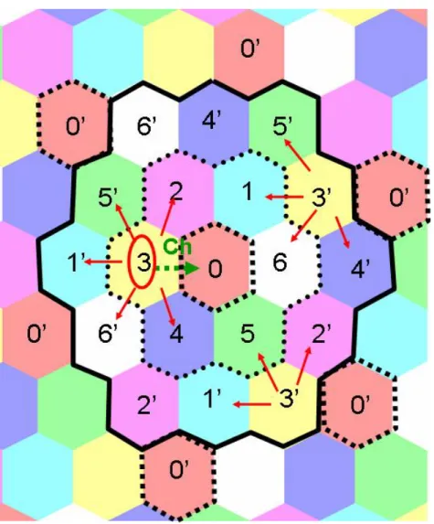
(21) Before introducing BDCL [22], we need make some definitions: 1. Base Cell : the cell that the self Base Station is located in, Cell 0 as the below Fig 2.5; 2. Neighboring Cell : the cells that are neighboring cells of Base Cell, Cell 1,2,…, 6 as the below Fig 2.5; 3. Adjacent Cell : the cells that are adjacent cells of Base Cell, Cell 1,2,…, 6, Cell 1’ , 2’ ,…, 6’ as the below Fig 2.5; 4. Co-Channel Cell : the cells that use the co-channels of Base Cell and is in the reuse distance of Base Cell, Cell 0’s as the below Fig 2.5. Fig 2.5 an example of regular cells. There are some characteristics for the network of regular cells [23]: 1. Channels are assigned by the base stations in the Cells; 2. Base stations do not measure any CIR (Carrier to Interference Ratio) parameters; 3. The network-wide assumption of the minimum reuse distance of a channel, which is the - 12 -.

(22) distance between one co-channel cell and another, is made. 4. The adjacent cells of the base cell are covered by the interference region of the base cell, and, the interference region is the region within the minimum reuse distance designated from the base station of the base cell; 5. The base station of the base cell can exchange information about channel usage status with the base stations of the adjacent cells; 6. A cell may assign a free channel that is not used by any adjacent cells to call in it. In the BDCL strategy, a set of nominal channels is assigned to each cell, and the co-channel cells use the same set of nominal channels. The major difference between BDCL strategy and FA strategy is that the base cell can borrow channels from the neighboring cells in the BDCL strategy. However, the borrowing operation may cause some side-effect; we will introduce it in the following example and illustrated as the above Fig 2.5: Step 1: Base Cell of Cell 0 attempt to borrow a channel from the neighboring cells; Step 2: Before borrowing a channel, Cell 0 has to check which neighboring cell is the richest cell that owns the most number of nominal channels not in use and not locked. Step 3: If the richest cell of Cell 0 is Cell 3, it has to borrow the channel that is not used by all adjacent cells of Cell 0 from Cell 3. Step 4: After making the decision of the borrowing channel, the co-channel cells of Cell 3 in the interference region of Cell 0, Cell 3 and Cell 3’s as Fig 2.5, have to be locked and to lock the channel in the proper directions to the neighboring cells of them. The locking of the channel means the cell that owns the channel as the nominal channel can not use it and the cell that does not own the channel can not borrow it. One more characteristic is that the set of the nominal channels for each cell have different priorities, from the highest to the lowest. Each cell uses the self channel with the highest priority of them and borrows the channel with the lowest priority of them from the richest neighboring cell.. - 13 -.

(23) Chapter 3 System Specification. To analyze the cost induced by call blocking and handoff dropping of the cellular system, we consider a mobile communication network with a cellular infrastructure. There are three major parts in this model: Base Station (BS), Mobile Station (MS) and the Channel. In the following, we describe these three components in detail, respectively.. 3.1 Base Station The geographical area controlled by a base station is called a cell. Each cell has one base station to make call admission control decisions for all mobiles that want to make a connection in it, either a new call or a handoff call from adjacent cells. The cellular system uses a dynamic channel allocation (BDCL) scheme, and each cell has a wireless link capacity C, but it can borrow channels from the neighboring cell if all capacity of it is in use. Because our model is based on information from adjacent cells such as call arrival rate, handoff rate and the number of ongoing connections, it is very important to maintain inter-BS communications. Thus we use the underlying network topology for base stations as shown in Fig. 3.1, where base stations are fully connected. In this topology, base stations can communicate directly, not via the mobile switching center (MSC), and each base station can perform the admission control test for newly-requested and handoff connections in its cell.. Fig. 3.1 Fully connected network architecture - 14 -.

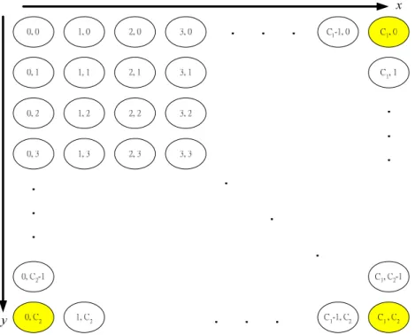
(24) 3.2 Mobile Station A mobile, while staying in a cell, communicates with another party, which may be a node connected to the wired network or another mobile, through the base station in the same cell. When it moves into an adjacent cell in the middle of a communication session, a handoff will enable the mobile to maintain connectivity to its communication partner, i.e., the mobile will start to communicate through the new base station, hopefully without noticing any difference. A handoff call could be dropped due to insufficient bandwidth available in the new cell, and in such a case, a cost occurs. Here, we preclude 1) delay-insensitive applications, which might be tolerate long handoff delays in case of insufficient bandwidth available in the new cell at the time of handoff and 2) soft handoff of the Code Division Multiple Access (CDMA) systems [13], [14], in which a mobile can communicate via two adjacent base stations simultaneously for a while before the actual handoff takes place. We use Guard Channel policy in the comparative case, where we propose to set aside some bandwidth in each cell for possible handoffs from its adjacent cells. This reserved bandwidth can be used only for handoffs from adjacent cells, but not for admitting newly-requested connections in the cell.. 3.3 Channel In our model, we assume that each cell can support up to C mobiles simultaneously, and each mobile use one channel to make the connection. As a result each cell has C channels. In our cellular system structure, all cells are surrounded by six cells. So this cell’s C channel and its adjacent cells’ total 6C channels evolve as a two-dimensional Markov chain as shown in Fig. 3.2 below. In Fig. 3.2, the first dimension is made of base cell’s channel state, where C1 is the fixed link capacity C. The second dimension is made of all adjacent cells’ total channel state, where C2 is six times of the fixed link capacity C. The total states of this two-dimensional Markov chain are C1 × C2. - 15 -.

(25) Fig. 3.2 Total states diagram of the two-dimensional Markov chain. - 16 -.

(26) Chapter 4 Problem Formulation by MDP in FA Strategy And Proposed Method. In this chapter, we introduce how to find the optimal policy under Markov Decision Process (MDP). Making a correct decision depends on cost function. We then use the policy-iteration method and state aggregation method to solve the problem of MINOBJ. In the case of single-service networks, Krishnan and Ott [15], and Lazarev and Starobinets [16] have proposed state dependent routing schemes with roots in Markov decision theory. We use the separable routing concept defined by Krishnan and Ott which is appropriately modified for the case of cellular networks. We also study the problem of call admission control where we follow Zachary’s procedure [17] to determine the cost of rejecting new calls and dropping handoff calls.. 4.1 Our Model The cell is described by a two-dimensional Markov chain with the following assumptions: 1. New call arrival in the base cell and adjacent cells are according to a stationary Poisson process with mean rate λ1 and λ2, respectively. 2. Departure rate of both new and handoff call is exponentially distributed with rate μ. 3. Call handoff form the base cell to adjacent cells and form adjacent cells to base cell are also exponentially distributed with rate h1 and h2, respectively. We consider a homogeneous system where each radio cell can support up to C calls, the cell state vector n(t) which provides the complete state description of the cell at any time instant is defined as. n(t ) = ( x, y ), ∀n ∈ N - 17 -. (4.1).

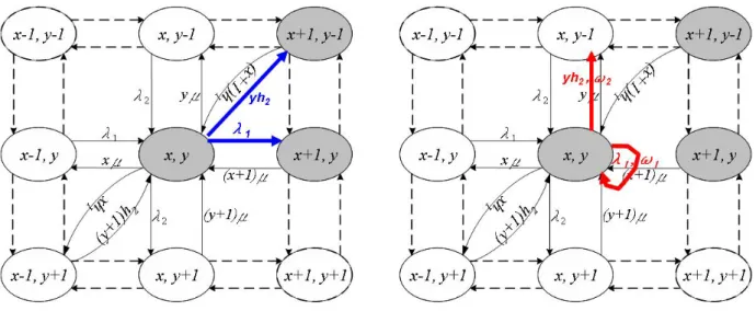
(27) where x is the number of calling mobiles in the base cell at time t, and y is the number of calling mobiles in all adjacent cells at time t. The cell space is denoted by N, which contains a finite but large number of states. The state transition rate diagram is shown in Fig. 4.1.. Fig. 4.1 State transition diagram. 4.2 Alternatives and Costs The MDP with costs has been the means to an end. This end is the analysis of decisions in sequential processes that are Markovian in nature [5]. We at first introduce alternatives and costs of sequential decision process and define them in this section. In our cell model, we have two alternatives when a new call (or a handoff call) comes: z. alternatives 1 : accept. z. alternatives 2 : reject (or drop). We then define that a cost ω1 (or ω2) is incurred when cell rejects (or drops) the arrival call. By these definitions, there are different behaviors with corresponding alternatives. In our case, we make a difference in Fig. 4.2 that cell admits a new (or handoff) call incur nothing but rejects (or drops) it with cost ω1 (or ω2). These analyses will help us to find the solution of the sequential decision process.. - 18 -.

(28) Fig. 4.2 Transition diagram with alternatives 1 and 2. 4.3 Our Policy-Iteration Method An optimal policy is defined as a policy that minimizes the cost. It is conceivable that we could find the cost for each of these decisions in order to find the policy with the least cost. We are interested in infinite-horizon systems and we know that the appropriate objective is the average cost optimization. It simply means that our goal is to minimize the expected rate of the cost of lost calls. Let us denote by Vπ(t) the lost revenue in the cell during the time interval [0, t] under the policy π ∈ П, where П is the set of all policies. Then, using the result from [5], we have the expected value E ⎡⎣Vπ ( t n0 = n ) ⎤⎦ = gπ t + vπ (n) + o(1), (t → ∞). (4.2). where n ∈ N is the cell state at time t = 0. In Markov decision theory, vπ(n) is the well-known relative value or cost of starting in state n0 = n. In Eq. (4.2), gπ represents the expected cost per unit time under the policy π on the original continuous-time scale. Since the system is ergodic, we may call gπ the gain of the process. The objective is to minimize the equilibrium expected cost per unit time, that is, gπ. The “small o” symbol o(1) means that for both the right hand side (RHS) and left hand side (LHS) of the equation go to infinity, and the difference goes to zero. Before to find the relative cost values vπ(n), we define two vectors. - 19 -.

(29) ⎡1 0 ⎤ ek ∈ℜ2 , ek = ⎢ ⎥ ⎣0 1 ⎦. (4.3). ⎡ −1 1 ⎤ f k ∈ℜ2 , f k = ⎢ ⎥ ⎣ 1 −1⎦. (4.4). Then, in the case of the departure of the call when the cell state is n, the immediately subsequent state dk(n) ∈ N is found as d k (n) = n − ek. (4.5). A new call admission decision needs to be made at call attempt epochs: either accept or reject. Denoting an alternative taken on the arrival of a call by πk(n) where n ∈ N is the current cell state. In the case of call rejection. π k ( n) = n. (4.6). If the new call is accepted, the subsequent state of the cell will be found as. π k (n) = n + ek. (4.7). A handoff call admission decision needs to be made at call cross the cell boundary epochs: either accept or drop. Use the same definition above, in the case of dropping a handoff call. π k (n) = n − ek. (4.8). If the handoff call is accepted, the subsequent state of the cell will be found as. π k ( n) = n + f k. (4.9). Now we start to introduce how to find the relative cost values vπ(n) for all n ∈ N. The same equation also governs the asymptotic behavior of the process if we assume that it has started immediately after the first event that has occurred after t = 0. This is because of the ergodic - 20 -.

(30) nature of the system, where the initial state has no effect on the asymptotic behavior of the process far enough in the nature. The first event is either a call termination or a new (handoff) call arrival. The expected time τ for the first event after t = 0 is given as 2. τ = 1/ γ , γ = ∑ ⎡⎣λk + nk ( μ + hk ) ⎤⎦. (4.10). k =1. where we used the memoryless property of the system. Writing Eq. (4.2) for a starting time t = 0 and a first event time t = τ (the latter one is conditional on the type of the first event), we obtain after some arrangements 2. 2. vπ (n) + gπ τ = τ ∑ nk μ vπ (d k (n)) + τ ∑ λk ⎡⎣δ k ( n, π k (n) ) ω1 + vπ (π k (n)) ⎤⎦ k =1. k =1. 2. + τ ∑ nk hk ⎡⎣δ k ( n − ek , π k (n) ) ω2 + vπ (π k (n)) ⎤⎦, ∀n ∈ N. (4.11). k =1. where δk( ⋅ ) is the Kronecker symbol as follows ⎧ 1, if n = π k (n) ⎩ 0, otherwise.. δ k ( n, π k (n) ) = ⎨. (4.12). In the system of linear Eq. (4.11), the unknown variables are vπ(n) for all n ∈N, and the gain of the process gπ. Obviously, the system has one more variable than the number of equations so that vπ( ⋅ )s can be determined up to an additive constant. To solve the system Eq. (4.11), we follow the standard procedure by setting vπ(0) = 0. Thus, we get the system 2. gπ = ∑ λk ⎡⎣δ k ( 0, π k (0) ) ω1 + vπ (π k (0)) ⎤⎦ k =1. 2. + ∑ nk hk ⎡⎣δ k ( 0, π k (0) ) ω2 + vπ (π k (0)) ⎤⎦. (4.13). k =1. 4.4 Our State Aggregation Method When using Gaussian elimination method to solve Eq. (4.11), we will face the same - 21 -.

(31) problem already described in section 2.5. The inverse matrix of transition probability matrix P is of complexity O(n3), which is impractical for large n. We take the Guard Channel policy mentioned in section 2.2 for an example. The threshold T will divide the states of the cell into three groups. From state 0 to T is of group one which can accept all kinds of calls. And from state ( T＋1 ) to ( C－1 ) is of group two which can accept only handoff calls. Note that there is a group three when the cell state is C. When in this group, no call will be accept due to unavailable of the channel. Thus we learn from this example that we can group states which are few steps reachable in the neighborhood. After that, we use the method like quantization to divide the one-dimensional Markov chain into even size, excluding the last state which is an independent group. Finally, in the case of taking adjacent cells’ states into consideration, the two-dimensional Markov chain can be grouped as shown in Fig. 4.3 below.. Fig. 4.3 Make two-dimensional Markov chain into smaller groups. - 22 -.

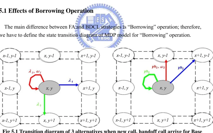
(32) Chapter 5 Modification from FA to BDCL by One-Step Policy And Update Rules of Policy with Time-varying MDP Parameters. In this chapter, we will introduce how we modify the previous MDP model of FA strategy to BDCL strategy by One-step Policy, which will make use of the previous computational result. Because the parameters of MDP model vary with time, we will introduce the update rules of time-varying MDP parameters to fit the actual system.. 5.1 Effects of Borrowing Operation The main difference between FA and BDCL strategies is “Borrowing” operation; therefore, we have to define the state transition diagram of MDP model for “Borrowing” operation.. Fig 5.1 Transition diagram of 3 alternatives when new call, handoff call arrive for Base Cell. As the above Fig 5.1, in BDCL model, there are three alternatives when a new call (or a handoff call) arrives: z. alternatives 1 : accept - 23 -.

(33) z. alternatives 2 : reject (block or drop). z. alternatives 3 : borrow. When a new call arrives, accepting the call will make a channel in use for Base Cell and therefore the state will transition right; blocking the call will not make any channel in use or released for Base Cell and therefore the state will self transition; borrowing a channel from the neighbor will make the neighboring cell one channel in use for Base Cell and therefore the state will transition down. It is illustrated as the above Fig 5.1. When a handoff call arrives, accepting the call will make a channel in use for Base Cell, a channel released for the neighboring cell and therefore the state will transition upward-right; dropping the call will make a channel released for the neighboring cell and therefore the state will transition up; borrowing a channel from the neighbor will make the neighboring cell one channel released for a neighboring cell, a channel in use for another and therefore the state will self transition. It is illustrated as the above Fig 5.1.. Fig 5.2 Transition diagram for alternatives 1, 2 and 3. - 24 -.

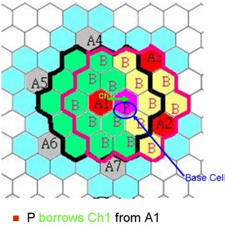
(34) As illustrated above in Fig 5.2, we will define a cost ω1 which is incurred with the alternative 2 when a new call arrives, a cost ω2 which is incurred with alternative 2 when a handoff call arrives, and a cost ω3 which is incurred with alternative 3 when a call (new call or handoff call) arrives. The cost ω3 is not fixed but varied with the condition of all adjacent cells, and ω3 is introduced by the effect of “Borrowing” operation on all adjacent cells. ω3 is derived online, and it depends on the condition which includes the channel to borrow and the states of all adjacent cells. After the borrowing, alternative 3 will cause the state transition of the adjacent cells of the base cell. There will be an example as illustrated as Fig 5.3 below.. Fig 5.3 Effect of borrowing operation on adjacent cells. If Cell P borrows Channel Ch1 from Cell A1, the state transitions of the adjacent cells will be illustrated below as Fig 5.4 and Fig 5.5. Fig 5.4 Example of effect by borrowing operation on adjacent cells - 25 -.

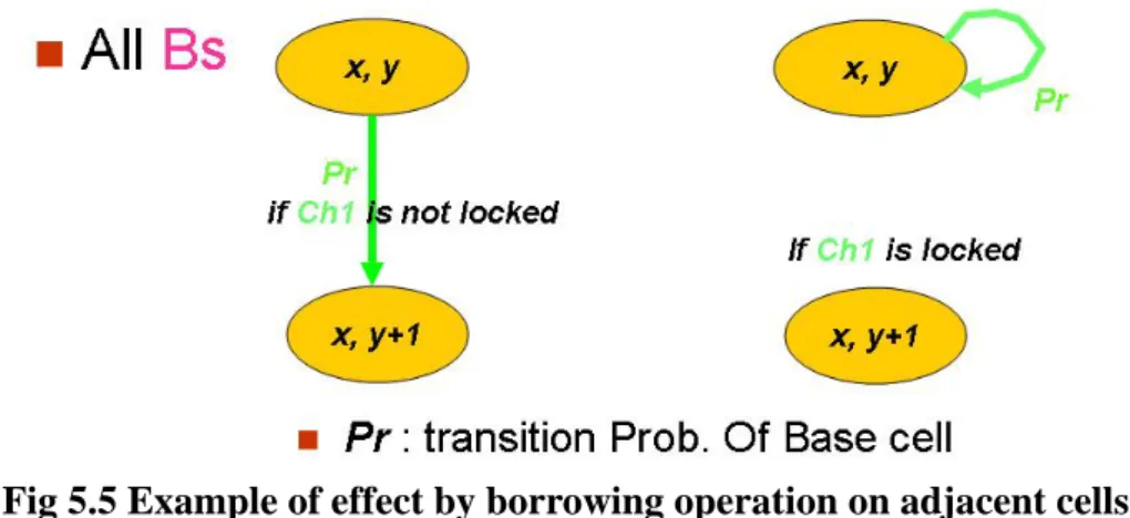
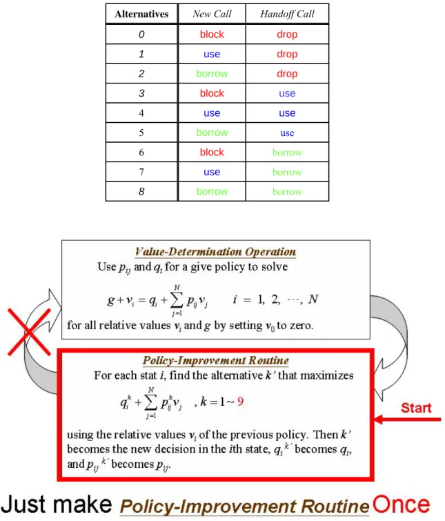
(35) Fig 5.5 Example of effect by borrowing operation on adjacent cells. Borrowing cost of ω3 is derived as Eq. (5.1) below: ⎧⎪Vi k (n) : Value of current state i current stage n for adjacent Cell k ⎨ k ⎪⎩V j (n + 1) : Value of next state j next stage n + 1 for adjacent Cell k N. ω3 = ∑ ⎡⎣V jk (n + 1) -Vi k (n) ⎤⎦, N : number of cells in the interference region k =1. (5.1). ⎧i = j , the selected channel to borrow is locked ⎨ ⎩i ≠ j , the selected channel to borrow is not locked. When a call (new call or handoff call) arrives, we have to check all channels of the neighboring cells and get the channel that will cause the least cost ω3. The channel that causes the least cost of ω3 is selected as the channel to borrow if alternative 3 is the best alternative to take.. 5.2 One-Step Policy for BDCL Strategy There are 9 Policies for both new calls and handoff calls, and it is listed as table 5.1 below. In order to get the One-step policy online, we facilitate the MDP computational result, which is derived offline, by FA strategy mentioned in chapter 4. And then we use the values of the states derived offline in FA strategy to get One-Step Policy, which is the improved policy. The improved policy means that the policy derived online is not the optimal policy but the improved one. The derivation of One-Step Policy is different from Policy Iteration Routine mentioned in chapter 3 because we just make Policy Improvement Routine once and not make Value Determination Routine. It is illustrated as Fig 5.6 below. It is proved that One-Step Policy although is not the optimal policy but it is closed to the optimal one [5], and since it just make Policy Improvement Routine once, it is also economical of computational resources. - 26 -.

(36) Table 5.1 Alternatives of One-Step Policy Alternatives. New Call. Handoff Call. 0. block. drop. 1. use. drop. 2. borrow. drop. 3. block. use. 4. use. use. 5. borrow. use. 6. block. borrow. 7. use. borrow. 8. borrow. borrow. Fig 5.6 One-Step Policy. One-Step-Policy improvement routine is illustrated above as Fig 5.6, we just make Policy-Improvement Routine once but run Value-Determination Operation.. 5.3 Update Rules of Policy with Time-varying MDP Parameters - 27 -.

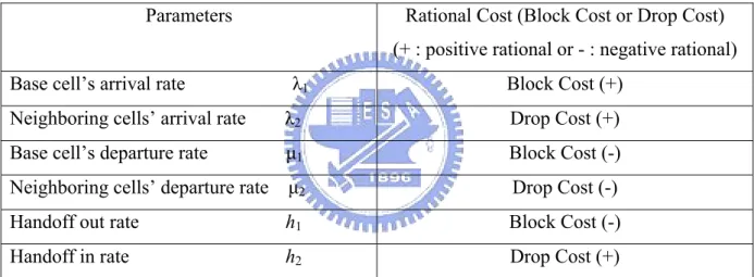
(37) There are six parameters in our MDP model, and they are λ1, λ2, μ1, μ2, h1 and h2. The six parameters of the actual system vary with time; therefore, we have to adjust them periodically to make our MDP model closer to the actual system and to get the more improved policy. The method how we adjust these parameters is to appreciate the system cost that is induced by rejecting calls (new calls or handoff calls) and the model cost that is one of the computational result in our MDP model, “gain”. The system cost is divided into two parts, and they are “Block Cost” that is the cost due to blocking new calls and “Drop Cost” that is due to dropping handoff calls. The update rule is derived by appreciating the data of the simulation result. We find that the six parameters may be rational to the either Block Cost or Drop Cost, and it is listed blow.. Table 5.2 Parameters update rules. Parameters. Rational Cost (Block Cost or Drop Cost) (+ : positive rational or - : negative rational). Base cell’s arrival rate. λ1. Block Cost (+). Neighboring cells’ arrival rate. λ2. Drop Cost (+). Base cell’s departure rate. μ1. Block Cost (-). Neighboring cells’ departure rate. μ2. Drop Cost (-). Handoff out rate. h1. Block Cost (-). Handoff in rate. h2. Drop Cost (+). The system cost is defined as Eq. (5.2), and it is the sum of the cost of rejecting calls. The model cost is defined as Eq. (5.2), and is the sum of the gain of the MDP model per update period. ⎧⎪model cost : ηt → Caverage (ηt ) , t : the t-th period of time ⎨ ⎪⎩system cost : Ct → C ( X t −1 , X t ). (5.2). Before the explanation of the update rules, we have to define the difference of model cost and system cost as Eq. (5.3) below: t. Yt = ∑ (Ci − ηi ), t : the t-th period of time. (5.3). i =1. - 28 -.

(38) Furthermore, the adjustment factor of parameters is defined as Eq. (5.4) below:. dt +1 =. Yt. , t : the t-th period of time. t. ∑η i =1. (5.4). i. The update rules for the six parameters are listed below as Eq. (5.5), Eq. (5.6), Eq. (5.7):. ω1 ⎧ t +1 ⎪λ1 = (1 + dt +1 × ω + ω ) × λ1 ⎧λ : base cell's arrival rate ⎪ 1 2 1 ,⎨ ⎨ ⎪λ t +1 = (1 + d × ω2 ) × λ ⎩λ2 : neighboring cells' arrival rate t +1 2 ⎪⎩ 2 ω1 + ω2. (5.5). ω1 ⎧ t +1 ⎪ μ1 = (1 − dt +1 × ω + ω ) × μ1 ⎧ μ : base cell's departure rate ⎪ 1 2 1 ,⎨ ⎨ ⎪ μ t +1 = (1 − d × ω2 ) × μ ⎩ μ2 : neighboring cells' departure rate t +1 2 ⎪⎩ 2 ω1 + ω2. (5.6). ω1 ⎧ t +1 ⎪h1 = (1 − dt +1 × ω + ω ) × h1 ⎧h : base cell's handoff-out rate ⎪ 1 2 1 ,⎨ ⎨ ⎪ht +1 = (1 + d × ω2 ) × h ⎩h2 : neighboring cells' handoff-in rate t +1 2 ⎪⎩ 2 ω1 + ω2. (5.7). The base station of each cell has to update the policy per period of time with the above update rules to ensure that the model is closer to the actual system. The update period is determined by how fast the system changes.. - 29 -.

(39) Chapter 6 Simulator and Results. 6.1 Simulator Settings 1. The size of the map for simulation is 12.12 km x 24.25 km. The map are composed of nodes that contain information about : i. the position : (x , y); ii. the type of the node : road or not; iii. the coverage of the cell. 2. There are 98 (14 X 7) cells on the map, and the radius of each cell is 2 km 3. Wrapped-around Map: when mobile reaches the boarder of the map, it will move to the opposite side boarder of the map. 4. There are 50 Channels per cell : the capacity of base cell (the number nominal channels C1) is 50, and the capacity of the neighboring cells C2 is 300. 5. The whole map is spread non-uniform traffic loading 6. Poisson Arrivals on the whole map with arrival rate λ (arrivals / cell / hour). Arrival Rate of mobiles in Base Cell : λ1 ; Arrival Rate of mobiles in Neighboring Cells : λ2. 7. Exponentially distributed service time per mobile with average service time 180 seconds per call. Departure Rate of mobiles in Base Cell : μ 1 ; Departure Rate of mobiles in Neighboring Cells : μ2. 8. Handoff rates are determined by the randomized number of mobiles in the base cell, the number of mobiles in the neighboring cells, the speeds of mobiles in the base cell and neighboring cells, and the road topology spread on the base cell and the neighboring cells, and so on. Handoff-in Rate : h1 ; Handoff-out Rate : h2. h1 and h2 are derived by measuring in Base Cell. 9. Mobiles move mainly in one direction and at speeds (20 ~ 90 km/hr) with 5% variance, and they do not move back unless there is no way to move forward, right, or left. 10. We define call failure rate: Call Failure Rate = Pb + (1-Pb) x Pd , Pb: Call Blocking Rate, Pd: Call Dropping Rate (6.1). - 30 -.

(40) Fig 6.1 Road Topology Example for Simulation - 31 -.

(41) 6.2 UML Statechart of Our Model We use UML(Unified Machine Language) to simulate the environment. The map is transformed from the simulator as illustrated in fig 6.1 above. The OMD (Object Main Diagram) is as illustrated in fig 6.2 below. When the simulation starts, one object of CellsGen generates objects of Map, of Cell, of Channel, and sets all links between Map-Cells, between Cell-Cell, between Cells-Channels. The object of Map generates the map and roads on the map in the beginning and produces objects of Mobile non-uniformly on the roads of the object of Map at the moment when the call comes. Objects of Mobile move along the roads generated by the object of Map, and make the handoff operation from one object of Cell to another when they move across the objects of Cell. The object of Cell has three jobs. First, it gets new calls and handoff calls from objects of Mobile. Secondly, it sets states of the objects of Channel. Finally, it informs the objects of Cell that are affected by the handoff operation, and keeps the list of using channels, the list of borrowing channels, and the list of borrowed channels. The objects of Channel are passive objects. They just own the records of states of themselves recorded by objects of Cell. The object of MDP owned by the object of Cell make calculation of Policy Iterations to decide the policy.. Fig 6.2 OMD of the Simulator. - 32 -.

(42) The State Chart of Mobile are illustrated as fig 6.3 below. When it is constructed, it will own a randomly generated service time which is exponentially distributed, the speed which is randomly selected from 20 km ~ 90 km. Its residual time is determined by the roads and the speed at which the object of Mobile moves.. Fig 6.3 State Chart of Mobile. The State Chart of Map is illustrated as Fig 6.4 below. When it is constructed, it produces the map in the beginning, and generates the inter-arrival time randomly with exponential distribution to determine when the object of Mobile is constructed. The State Chart of Cell is illustrated as Fig 6.5 below. It receives events evIn which include new call events from objects of Mobile, and handoff-in call events from objects of Cell. It also receives events evOut which include call ending events from objects of Mobile and handoff-out events from objects of Cell. It also periodically updates parameters including Base Cell arrival rateλ1 , Neighboring Cell arrival rateλ2, Base Cell departure rateμ1, Neighboring Cell departure rateμ2, Handoff-out rate h1, and Handoff-in rate h2.. - 33 -.

(43) Fig 6.4 State Chart of Map. Fig 6.5 State Chart of Cell. Because there are total 50 × 300 states which is to difficult to compute and not efficient in real-time, we use the aggregation method mentioned to group states into smaller groups. In our model, we choose total 6 × 11 states as shown in Table 6.1 below which is a compromise between computing complexity and the difference of the result derived. After the offline policies are determined, the values of all states are derived. With the values of the states, we will then determine the online policies by One-Step policy when events evIn occur. - 34 -.

(44) Note that the last column and row (with gray background) of the table is made of only one single state. Because no matter there is a new call or a handoff call arrives in that state, it will not be accepted due to unavailable of the channel. And the information of adjacent cells’ state will be update periodically. When the policy is derived, each cell’s base station can make call admission control according to nine actions listed in Table 6.2 below.. Table 6.1 Aggregation of total states Base Cell’s Group Cell’s States. Adjacent Cells’ Group. (after aggregation). 0~9 10~19 20~29 30~39 40~49 50 1. 2. 3. 4. 5. 6. 0~29. 1. 0. 1. 2. 3. 4. 5. 30~59. 2. 6. 7. 8. 9. 10. 11. 60~89. 3. 12. 13. 14. 15. 16. 17. 90~119. 4. 18. 19. 20. 21. 22. 23. 120~149 5. 24. 25. 26. 27. 28. 29. 159~179 6. 30. 31. 32. 33. 34. 35. 180~209 7. 36. 37. 38. 39. 40. 41. 210~239 8. 42. 43. 44. 45. 46. 47. 240~269 9. 48. 49. 50. 51. 52. 53. 270~299 10. 54. 55. 56. 57. 58. 59. 60. 61. 62. 63. 64. 65. 300. 11. - 35 -.

(45) Table 6.2 Alternatives of base cell’s states. Alternatives. New Call Handoff Call. 0. block. drop. 1. use. drop. 2. borrow. drop. 3. block. use. 4. use. use. 5. borrow. use. 6. block. borrow. 7. use. borrow. 8. borrow. borrow. 6.3 Simulation Results BDCL Block Rate(Fixed Policy). 0.7000 0.6000. Prob. 0.5000. Normal BR Policy BR Guard BR. 0.4000 0.3000 0.2000 0.1000 0.0000 Load50. Load70. Load90. Load100. Load150(5- Load150(5- Load200(5- Load200(540) 45) 50) 60) Load(%). BDCL Block Rate(Policy pdated per 15 sec). 0.6000 0.5000. Prob. 0.4000. Normal BR. 0.3000. Policy BR. 0.2000. Guard BR. 0.1000 0.0000 Load50. Load70. Load90. Load100 Load150(5Load(%) 40). Load150(545). Load200(550). Load200(560). Fig 6.6 Call Block Rate of different method under different loads - 36 -.

(46) Call blocking Rate is illustrated above as Fig 6.6, there are three methods of BDCL, which are BDCL without call admission control, call admission control by MDP, call admission by Guard Channel Policy. They are simulated under different loads and cost (block cost-drop cost), 50% (5-30), 70% (5-30), 90% (5-30), 100% (5-30), 150% (5-40) ,150% (5-45), 200% (5-50), 200% (5-60). We also simulated it with update periodically and without it. The result shows that Block Rate of our MDP method no matter with periodic policy update or not is lower than that of Guard Channel of BDCL when traffic load is under 100%. However, Block Rate of our MDP method without periodic policy update is higher than that of Guard Channel policy of BDCL when traffic load is greater than 100%, but Block Rate of our MDP method with periodic policy update is lower than that of Guard Channel policy of BDCL. We can conclude that our MDP method with periodic policy update gets better efficiency than Guard Channel policy of BDCL.. BDCL Drop Rate(Not Updated) 0.3500 0.3000 0.2500. Normal DR. 0.2000. Prob. Policy DR. 0.1500. Guard DR. 0.1000 0.0500 0.0000 Load50. Load70. Load90. Load100. Load150(540) Load(%). Load150(545). Load200(550). Load200(560). BDCL Drop Rate Prob. 0.3500. 0.3000. Normal DR. 0.2500. Policy DR. 0.2000. Guard DR 0.1500. 0.1000. 0.0500. 0.0000. Load50. Load70. Load90. Load100. Load150(5-40) Load150(5-45) Load200(5-50) Load200(5-60). Fig 6.7 Call Drop Rate of different method under different loads - 37 -. Load(%).

(47) Call Dropping Rate are illustrated above as Fig 6.7. The result shows that call drop rate of our MDP method without periodic policy update is almost the same as that of Guard Channel policy of BDCL. However, call drop of our MDP method with periodic policy update is higher than that of Guard Channel policy of BDCL. We can conclude that our method with periodic policy update gets worse efficiency than Guard Channel policy of BDCL and our method without periodic policy update.. BDCL Failure Rate(Not Updated). 0.7000 0.6000. Prob. 0.5000 0.4000 0.3000. Normal FR. 0.2000. Policy FR Guard FR. 0.1000 0.0000 Load50. Load70. Load90. Load100. Load150(5-40) Load150(5-45) Load200(5-50) Load200(5-60). Load(%). BDCL Failure Rate. 0.7000 0.6000. Prob. 0.5000 0.4000 Normal FR Policy FR Guard FR. 0.3000 0.2000 0.1000 0.0000 Load50. Load70. Load90. Load100. Load150(540) Load(%). Load150(545). Load200(550). Load200(560). Fig 6.8 Call Failure Rate of different method under different loads. Call Failure Rate is illustrated above as Fig 6.8. The result shows that call failure rate of our MDP method without periodic policy update is higher than that of Guard Channel policy of BDCL under all traffic loads. However, call failure rate our MDP method with periodic is lower than that of Guard Channel policy under traffic load 100%, but it is higher under traffic. - 38 -.

(48) load higher than 100%. We conclude that the efficiency of our method gets better under traffic 100% than Guard Channel policy of BDCL.. Cell 16. Cell 57. Fig 6.9 Map of road topology in Cell 16, Cell 57 and Cell 62. Fig 6.10 Parameters update for load 70 Cost 5-30 of period 15 sec. - 39 -. Cell 62.

(49) Fig 6.11 Parameters update for load 70 Cost 5-30 of period 60 sec. Fig 6.12 Parameters update for load 70 Cost 5-30 of period 120 sec. - 40 -.

(50) Fig 6.13 Parameters update for load 70 Cost 5-30 of period 180 sec. Fig 6.14 Parameters update for load 70 Cost 5-30 of period 240 sec. - 41 -.

(51) Fig 6.15 Parameters update for load 70 Cost 5-30 of period 300 sec. Fig 6.16 Parameters for load 70 Cost 5-30 without periodic update. - 42 -.

(52) As illustrated above in Fig 6.10, Fig 6.11,…, Fig 6.16, they are curves of six parameters of Cell 16, of Cell 57 and of Cell 62 with time varying under different policy update periods, which are 15 seconds, 60 seconds, 120 seconds, 180 seconds, 240 seconds, 300 seconds and no policy update. Cell 16, as illustrated above in Fig 6.9, is the cell with the most crowded road topology among those three cells; Cell 57 is the medium one; Cell 62 is the one with the least crowded road topology. The above Figures show that the six parameters of more crowded road topology vary more severely with time and vary more frequently with more frequent policy update.. Fig 6.17 Average cost of Load 70 Cost 5-30 with different update periods. - 43 -.

(53) Fig 6.18 Average cost of Load 90 Cost 5-30 with different update periods. Fig 6.19 Average cost of Load 100 Cost 5-30 with different update periods. - 44 -.

(54) Fig 6.20 Average cost of Load 150 Cost 5-40 with different update periods. Fig 6.21 Average cost of Load 150 Cost 5-45 with different update periods. - 45 -.

(55) Fig 6.22 Average cost of Load 200 Cost 5-50 with different update period. Fig 6.23 Average cost of Load 200 Cost 5-60 with different update period. - 46 -.

(56) As illustrated above in Fig 6.17 and Fig 6.18, the result shows that the average cost is not lower with more periodic policy update. In Fig 6.17, it is simulated under traffic load 70% for different policy update periods, and the average cost of update period 120 seconds is the lowest one among those of other update periods. In Fig 6.18, it is simulated under traffic load 90% for different policy update periods, and the average cost of update period 180 seconds is the lowest one among those of other update periods. It means that the more frequent policy update does not get the better efficiency. From Fig 6.19, Fig 6.20,…, Fig 6.23 illustrated above, they are simulated under traffic loads of 100%, 150% and 200% for different policy update periods. Those figures show that the average cost without policy update is lower under traffic loads over 100%. The efficiency is better if we do not update policy under over-loaded traffic. Moreover, From Fig 6.17 to Fig 6.23, we find that the average cost with more frequent policy update does not adjust so severely with great dumping. The curve of those average costs is smoother with more frequent policy update.. - 47 -.

(57) Chapter 7 Conclusion. In the thesis, we simulated the call admission control problem in cellular networks with BDCL strategy by One-Step Policy under the environment of road topology. The result shows that the efficiency of call failure rate is better under traffic load of less than 100% than that of Guard Channel Policy of BDCL. However, if the traffic load is over 100%, the efficiency gets worse than Guard Channel Policy of BDCL. We suppose that our method would preserve some channels to borrow before the system reaches the convergence, but this phenomenon causes the waste of channels and therefore, the efficiency gets worse than Guard Channel Policy of BDCL. As we mentioned, the borrowing takes costs. In the aspect of periodic policy update of six parameters, the result shows that the efficiency of call failure rate with policy update is better than that without policy update. However, it causes the efficiency of call dropping rate worse. This is the trade-off between update and no update.. - 48 -.

(58) References [1] S. Tekinay and B. Jabbari, “Handover and Channel Assignment in Mobile Cellular Networks,” IEEE Commun. Mag., vol. 29, no. 11, Nov. 1991. [2] E. C. Posner and R. Guerin, “Traffic Policies in Cellular Radio that Minimizing Blocking of Handoff Calls,” in Proc. 11th Teletraffic Cong. (ITC 11), Kyoto, Japan, Sept. 1985. [3] S. Choi and K. G. Shin, “Adaptive Bandwidth Reservation and Admission Control in QoS-Sensitive Cellular Networks,” IEEE Trans. Parallel and Distributed Sys., vol. 13, no. 9, pp. 882–897, Sep. 2002. [4] R. Ramjee, D. Towsley, and R. Nagarajan, “On Optimal Call Admission Control in Cellular Networks,” Wireless Networks Journal, vol. 3, no. 1, pp. 29-41, March 1997. [5] R. A. Howard, Dynamic Programming and Markov Processes, MIT Press, 1960. [6] D. P. Bertsekas, Dynamic Programming and Optimal Control, vol. 2, 2nd edition, Athena Scientific, Belmont, Massachusetts, 2000. [7] D. P. Bertsekas, Dynamic Programming: Deterministic and Stochastic Models, Prentice-Hall, Englewood Cliffs, NJ, 1987. [8] D. Hong and S. S. Rappaport, “Traffic Model and Performance Analysis for Cellular Mobile Radio Telephone Systems with Prioritized and Nonprioritized Handoff Procedures,” IEEE Trans. on Vehicular Tech., vol. 35, no. 3, pp. 77-92, Aug. 1986. [9] B. L. Miller, “A Queuing Reward System with Several Customer Classes,” Management Science, vol. 16, no. 3, pp. 234-245, 1969. [10] M. L. Puterman and M. C. Shin, “Modified Policy Iteration Algorithms for Discounted Markov Decision Problems,” Management Science, vol. 24, no. 11, pp. 1127-1137, Jul. 1978. [11] M. L. Puterman and M. C. Shin, “Action Elimination Procedures for Modified Policy Iteration Algorithms,” Operations Research, vol. 30, no. 2, pp. 301-318, 1982. [12] E. L. Porteus, “Overview of Iterative Methods for Discounted Finite Markov and Semi-Markov Decision Chains,” in Recent Developments in Markov Decision Process, R. Hartley et. al. (eds.), New York: Academic Press, 1980. [13] D. Collins and C. Smith, 3G Wireless Networks, McGraw-Hill, 2001. [14] A. J. Viterbi, CDMA: Principles of Spread Spectrum Communication, Reading, Mass.: Addison-Wesley, 1995. [15] T. J. Ott and K. R. Krishnan, “State Dependent Routing of Telephone Traffic and the Use - 49 -.