Propagation Effects on Outdoor MIMO Capacity
:
:
Propagation Effects on Outdoor MIMO Capacity
Student : Ming-Zhe Tsai
Advisor : Dr. Jenn-Hwan Tarng
A Thesis
Submitted to Department of Communication
College of Engineering
National Chiao Tung University
in Partial Fulfillment of the Requirements
for the Degree of
Master of Science
in
Communication Engineering
July 2004
Hsinchu, Taiwan, Republic of China
-Propagation Effects on Outdoor MIMO Capacity
Student
Ming- Zhe Tsai Advisor
Dr. Jenn- Hwan Tarng
Department of Communication Engineering
National Chiao Tung University
Abstract
Large capacity is obtained via the potential decorrelation among MIMO spatial radio channels. A fully correlated MIMO radio channel only offers one equivalent subchannel for transmission and a completely decorrelated MIMO spatial radio channel potentially offer multiple subchannels depending on the antenna array arrangement and propagation effects. In this paper, effects of propagation conditions such as LOS, OLOS and NLOS, propagation distance, local scatterer distributions, signal bandwidth and antenna array element spacing on 4x4 MIMO capacity are investigated through extensive measurement in macrocellular environments. It is found that the rms AOA (Angle-of-Arrival) and number of multipath components (MCPS) are the two fundamental parameters to affects the capacity. Environments under rich scattering signals such as NLOS condition and existing of local scatterers exhibiting a high rms angular spread of AOA ensures a high probability of achieving independent fading and hence boosts capacity. The increase of the array element spacing decreases the correlation among spatial channels, i.e., increasing the capacity. It is also found that the increase of signal bandwidth will increase the signal resolution and hence number of MPCs increases, which enhances the capacity. It seems that the capacity is independent of propagation distance and angular spread of AOD.
Contents
Contents... VI List of Figures ... VII List of Tables ... ... ... ... IX
Chapter 1 ... 1
Introduction ... 1
Chapter 2 ... 5
Capacity Estimation of MIMO Systems ... 5
2.1 Capacity Formulas ... 5
2.2 Spatial Correlation Coefficient... 9
2.3 Eigenanalysis on MIMO channel...11
2.4 MIMO LOS Channels ... 16
Measurement campaign and set-up ... 19
3.1 Measurement Set-up... 19
3.2 Measurement Campaign... 21
3.3 Measurement data extraction ... 31
Propagation and Antenna Arrangement Effects on MIMO Capacity... 37
4.1 Propagation effect ... 37
4.1.1 Measured result analysis ... 37
4.1.2 Comparison among different routes ... 42
4.2 Element spacing effect ... 48
4.2.1 Measurement Result Analysis ... 48
4.2.2 Computation with the Hybrid model... 53
4.2.3 Comparison ... 56
4.3.1 Bandwidth Effect... 60
4.3.2 Angle Spread Effect ... 63
Conclusion... 71
List of Figures
Fig 1 MIMO system configuration ... 2 Fig 2-1 Shannon capacity as function of number of transmitter and receiver antennas 9 Fig 2-2 Transmission from three (N) transmit antennas to two (M) receive antennas.14 Fig 2-3 N-input M-output configuration ... 18 Fig 3-1 System diagram of the RUSK vector channel sounder ... 21 Fig 3-2 RUSK vector channel sounder. (a) Transmitting unit. (b) Receiving unit. .... 21 Fig 3-3 Measurement sites in the NCTU campus ... 24 Fig 3-4 The field strength distribution of propagation, power delay profile and power
azimuth profile for LOS of route no.1 in the left straight side, the ones which transmitter and receiver are interchanged shown in the right straight. ... 26 Fig 3-5 Time Averaged Delay-Azimuth Spectrum of measurement of route no.1... 27 Fig 3-6 (a) Field strength distribution of route no.2 and the Power Delay Profile and
Power Azimuth Profile of route no.2 (b) Time Averaged Delay-Azimuth Spectrum of measurement of route no.2 ... 28 Fig 3-7 (a) Field strength distribution of route no.3 and the Power Delay Profile and
Power Azimuth Profile of route no.3 (b) Time Averaged Delay-Azimuth Spectrum of measurement of route no.3 ... 29 Fig 3-8 (a) Field strength distribution of route no.4 and the Power Delay Profile and
Power Azimuth Profile of route no.4 (b) Time Averaged Delay-Azimuth Spectrum of measurement of route no.4 ... 30 Fig 3-9 The impulse response of (a) top (b) bottom left (c) bottom right figure
presents the measurement during different observation time... 32 Fig 3-10 The frequency response (a) and impulse response (b) of the channel... 34 Fig 4-1 The CDF of the measured MIMO capacity for LOS (*), OLOS (o) and NLOS
( ) conditions along route no.1. . ... 38 Fig 4-2 capacity versus rms angular spread of AOA for LOS (*), OLOS (o) and NLOS ( ) conditions... 38 Fig 4-3 The histogram of MIMO capacity for (a) LOS, (b) OLOS and (c) NLOS
conditions. ... 40 Fig 4-4 The CDF of the measured MIMO capacity for LOS (*), OLOS (o) and NLOS
( ) conditions along route no.2. ... 40 Fig 4-5 The CDF of the measured MIMO capacity for LOS (*), OLOS (o) and NLOS
( ) conditions along route no.3. ... 41 Fig 4-6 The CDF of the measured MIMO capacity for LOS (*), OLOS (o) and NLOS
( ) conditions along route no.4. ... 41 Fig 4-7 (a) The CDF of capacity of LOS in each route, (b) the CDF of capacity of
OLOS in each site and (c) the CDF of capacity of NLOS in each site. ... 43 Fig 4-8 The capacity variation of different propagation distance D from measurement
with standard deviation of the capacity... 45 Fig 4-9 The CDF of capacity for different propagation distance applying hybrid model
... 46 Fig 4-10 The capacity variation of LOS along different routes with standard deviation
of capacity ... 46 Fig 4-11 The computed CDF of the MIMO capacity for routes no.1-4 by using the
hybrid model. ... 47 Fig 4-12 The averaged MIMO capacity for each route... 47
Fig 4-14 The capacity variation under LOS with MIMO element spacing for route
no.1 with standard deviation of capacity... 49
Fig 4-15 The CDF of different element spacing for LOS along route no.1. ... 49
Fig 4-16 histogram corresponding to MIMO capacity for LOS along route no.1 with (a) 10 (b) 20
(c) 30 ... 51
Fig 4-17 (a) The CDF of different element spacing for LOS along route no.2. ... 51
(b) The CDF of different element spacing for LOS along route no.3. ... 52
(c) The CDF of different element spacing for LOS along route no.4. . ... 52
Fig 4-18 The averaged capacity with MIMO element spacing for all measurements 53 Fig 4-19 (a) CDF of capacity applying hybrid model for different element spacing. (b) CDF of capacity between 6 propagation under the condition of scatter radius 2m and different number of local scatterers and propagation without considering local scatter. (c) CDF of capacity for different scatterer radius 56 Fig 4-20 The comparison of CDF of capacity of different element spacing between the measurement and hybrid model for (a) route no.1, (b) route no.2, (c) route no.3 and (d) route no.4, respectively. ... 59
Fig 4-21 The capacity versus signal bandwidths for three propagation conditions LOS, OLOS and NLOS along route no.1 ... 61
Fig 4-22 The maximum, minimum and mean values for three propagation conditions LOS, OLOS and NLOS of different bandwidth along route no.1... 61
Fig 4-23 The capacity versus signal bandwidths for three propagation conditions LOS, OLOS and NLOS along route no.1 ... 62
Fig 4-24 The capacity versus signal bandwidths for three propagation conditions LOS, OLOS and NLOS along route no.3. ... 62
Fig 4-25 The capacity versus signal bandwidths for three propagation conditions LOS, OLOS and NLOS along route no.4. ... 63
Fig 4-26 (a) capacity versus rms azimuth spread of AOA for route no.1 ... 67
(b) capacity versus rms azimuth spread of AOA for route no.2... 67
(c) capacity versus rms azimuth spread of AOA for route no.3 ... 68
(d) capacity versus rms azimuth spread of AOA for route no.4... 68
Fig 4-27 The Delay-Azimuth Spectrum of measurement data and the resolved scattered wave (*) on the time and azimuth resolution and CDF of capacity for subchannels and eigenvalue distribution of measurement for (a) route no.2 (b) route no.3 and (c) route no.4... 70
List of Tables
Table 1-Descriptions of the propagation environment at each route. ... 23 Table 2-Mean capacity [bps/Hz] for three propagation, which has three kinds of
element spacing of 4 routes... 60 Table-3 The mean capacity, standard deviation of capacity, standard deviation of rms
of azimuth spread of AOA and standard deviation of rms of azimuth spread of AOD for all measurement sites. ... 65
Chapter1 Introduction
Chapter 1
Introduction
The explosive growths of the wireless industry and the internet are creating a huge market opportunity for wireless data access. Limited internet access at low speeds (a few tens of kilo-bits per second at most) is already available as an enhancement to some second-generation (2G) cellular systems. However those systems were originally designed with the sole purpose of providing voice services and at most short messaging, but not high-speed data transfers. To increase system capacity of mobile networks of 3G and B3G communication systems, smart antennas have utilized SDMA (Space Division Multiple Access) technique to increase signal gain and to reduce interference. Multiple-input-multiple-output (MIMO) system, which has multiple antenna elements at both the transmitter and receiver, is illustrated in Fig. 1. The idea behind MIMO is that the signals on the transmit antennas and that of the receive antennas are combined [1] in such a way that the quality (bit error rate) or the data rate (bit/sec) of the communication will be improved. Such an advantage can be used to increase both the networks quality and the operator s revenues significantly. A core idea in MIMO systems is space-time signal processing in which time dimension (the natural dimension of digital communication data) is complemented with the spatial dimension inherent in the use of multiple spatially distributed antennas.
antennas , a popular technology using antenna arrays for improving wireless transmission dating back several decades. Conventional smart antenna systems yield a capacity enhancement or range extension over conventional fixed beam antenna installations by focusing their beam patterns towards an addressed volume associated with the signaling space of the desired traffic channel.
Fig. 1 MIMO system configuration
Large capacity is obtained via the potential decorrelation in the MIMO radio channel within the confine of the limited radio spectrum allocated to these systems, which can be exploited to create many parallel subchannels. However, the potential capacity gain is highly dependent on the multipath richness in the radio channel, since a fully correlated MIMO channel only offers one subchannel, while a completely decorrelated channel offers multiple subchannels depending on the antenna configuration-the most striking property of MIMO systems is the ability to turn multipath propagation, usually a pitfall of wireless transmission, into an advantage for increasing the user s data rate. [2]
factors, none more than propagation and antenna arrangement. Measurement of outdoor MIMO channels have been reported in [3] without providing insights into the relation between the channel structure, the corresponding capacity and the propagation. The influence of spatial fading correlation at either transmit or the receive side of a wireless MIMO radio link has been addressed in [4]. While the models used in [4] are simple and allow gaining insight into the impact propagation conditions on MIMO capacity they assume that only spatial fading correlation is responsible for the rank structure of the MIMO channel. In practice, however, the realization of high MIMO capacity in actual radio channels is sensitive not only to the fading correlation but also to the structure of scattering in the propagation [5]. Ref [6] provides an approach modeling MIMO channel to investigate the impact of MIMO capacity on more realistic channel and several key questions regarding outdoor MIMO channels, including (1) What is the capacity of a typical outdoor MIMO channel? (2) What are the key propagation parameters governing the capacity behavior? (3) Under what conditions do we get a high rank MIMO channel (and hence high capacity)? (4) What is a simple analytical model describing the capacity behavior of outdoor MIMO wireless channels accurately? Environment under rich scattering signals exhibiting a high azimuth spread ensures a high probability of achieving independent fading and hence boosts capacity. Measurements of MIMO channels are therefore necessary in order to characterize the performance of these systems in real environments.
In this paper, we analyze the factors of impact on capacity for different sites and try to find the answers to the above questions. We use a physical-statistical spatio-temporal channel model, which consists of a site-specific deterministic model with a geometrically based single bounce statistical model.
The paper is organized as following: In chapter 2, the fundamental theory of MIMO system will be introduced and the governing condition of obtaining high capacity is introduced. In Chapter 3, measurement campaign is described and channel multipath parameters such as AOA, AOD and frequency response extracted from measurement data. In chapter 4, the impact of propagation and antenna arrangement on capacity are analyzed. In chapter 5, the conclusion is presented
chapter2 Capacity Estimation of MIMO systems
Chapter 2
Capacity Estimation of MIMO Systems
Todays inspiration for research and applications of wireless MIMO systems was triggered by the initial Shannon capacity results obtained independently by Bell Labs researchers E. Telatar and J. Foschini, further demonstrating the seminal role of information theory in telecommunications. The analysis of theoretical capacity gives information on how the channel model or the antenna setup itself may influence the transmission rate. It helps the system designer benchmark transmitter and receiver algorithm performance. Here we examine the capacity aspects of MIMO systems compared with single input single output (SISO) and single input multiple output (SIMO) and multiple input single output (MISO) systems.
2.1 Capacity Formulas
A. Shannon capacity of wireless channels
Given a single channel corrupted by an additive white Gaussian noise (AWGN), at a level of SNR denoted by , the capacity (rate that can be achieved with no constraint on code or signaling complexity) can be written as
2 log (1 ) bps/Hz SISO C
(1)
power to obtain double capacity (To go from 1bps/Hz to 11bps/Hz the transmitter power must be increased by 1000 times). In practice wireless channels are time-varying and subject to random fading. In this case we denote h the unit-power complex Gaussian amplitude of the channel at the instant of observation. The capacity, written as
2 2 log (1 ) bps/Hz SISO C h
(2)
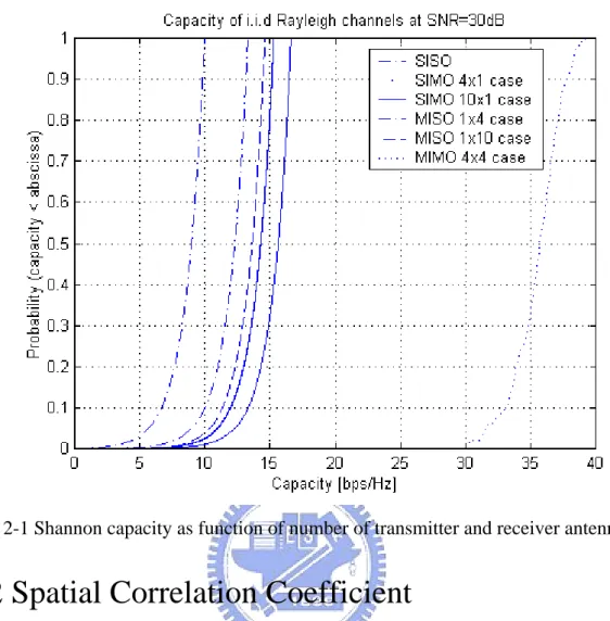
becomes a random quantity, whose distribution can be computed. The cumulative distribution of this 1x1 case (one antenna on transmit and one on receive) is shown on the left in Fig.2-1 We notice that the capacity takes, at times, very small values, due to fading events.
B. Multiple antennas at one end
Given a set of M antennas at the receiver (SIMO system), the channel is now composed of M distinct coefficients h [ ;h ; h0 1 ; hM-1] where hi is the channel amplitude from the transmitter to the i-th receiver antenna. The expression for the random capacity can be generalized to
2 1 1 lo g ( H ) S IM O M M x M x C I h h
(3)
where [ ]Hrepresents Hermitian transposition, can be approximated as
2 log (1 ) bps/Hz SIMO C M
(4) M is the number of the receiver. Compared to the capacity of SISO system
2
lo g (1 ) b p s/H z
S ISO
C
It shows that slow logarithmic growth of the bandwidth efficiency limit.
In Fig. 2-1, we see the impact of multiple antennas on the capacity distribution with 4 and 10 antennas respectively. This is due to the spatial diversity, which reduces fading and the higher SNR of the combined antennas.
However going from 4 to 10 antennas does not give very significant improvement as spatial diversity benefits quickly level off. The increase in average capacity due to SNR improvement is also limited because the SNR is increasing inside the log function in (3). We also show that the results obtained in the case of multiple transmit antennas and one receive antenna, 4x1 and 10x1 when the transmitter does not know the channel in advance. In such circumstances the multiple transmit antennas cannot beamform blindly. Conventional multiple antenna systems are good at improving the outage capacity performance, attributable to the spatial diversity effect but this effect saturates with the number of antennas.
C. Capacity of MIMO links
We now consider a full MIMO link as Fig. 1 with N transmit antennas and M receive antennas respectively. The channel is represented by a matrix of size M x N with random elements denoted by HM xN , we have the now famous capacity equation [1] M IM O 2 C lo g (IM H H H ) b p s /H z N
(5) when 1 HHH IN N , (5) can be approximated as 2 lo g (1 ) b p s /H z k = m in { M ,N } M IM O C k
(6) boosting compared to SISO channels and fast growth compared to SIMO channels
Foschini [1] and Telatar [3] both demonstrated that the capacity in (5) grows linearly with k=min (M, N) rather than logarithmically. This result can be intuited as follows the determinant operator yields a product of min(M,N) nonzero eigenvalues of its (channel-dependent) matrix argument, each eigenvalue characterizing the SNR
using a pair of right and left singular vectors of the channel matrix as transmit and receive antenna weights, respectively. Thanks to the properties of the log, the overall capacity is the sum of capacities of each of these modes, hence the effect of capacity multiplication. Clearly, this growth is dependent on properties of the eigenvalues. If they decayed away rapidly then linear growth would not occur. However, the eigenvalues have a known limiting distribution and tend to be spaced out along the range of this distribution. Hence, it is unlikely that most eigenvalues are very small and the linear growth is indeed achieved. In theory and in the case of idealized random channels, limitless capacities can be realized provide that we can afford the cost and space of many antennas and RF chains. In reality the performance will be dictated by the practical transmission algorithms selected and by the physical channel characteristics.
Applying MIMO techniques to wireless communication to meet the anticipated demand for high bit rate, real time services within limited bandwidths. MIMO propagation channel asymptotically gives M x N diversity and min (M, N) orthogonal communication channels for fully uncorrelated antennas. A large number of parallel channels is attractive since they are capable of carrying parallel information in the same bandwidth. The eigenvalue decomposition deduced from the propagation channel matrix (M x N) is an important parameter in this context because it determines the effective number of available parallel subchannels. Next we will introduce the concept of eigen-analysis on MIMO channel, a matrix solution leads itself to an analytical approach where the eigenvalues of the transmission system lead to a definition of the maximum gain as the largest eigenvalue.
Fig. 2-1 Shannon capacity as function of number of transmitter and receiver antennas
2.2 Spatial Correlation Coefficient
The complex correlation coefficient is a complex number that is less than unity in absolute value. Let a, b be two complex random variables, the complex correlation coefficient of a and b is defined as
* * 2 2 2 2
[
]
[ ] [ ]
,
E ab
E a E b
a b
E a
E a
E b
E b
where * denotes the complex conjugate operation. It is assumed that all antenna elements in the two arrays have the same polarization and the same radiation pattern. The spatial complex correlation coefficient at the BS between antenna m1 and m2 is
given by
,
BSh
h
(7)
where < a, b> computes the correlation coefficient between a and b. The spatial complex correlation coefficient observed at the MS is similarly defined as
1 2 1
,
2MS
m m
h
mnh
mn(8)
Given (7) and (8), we can define the following symmetrical complex correlation Matrices 11 12 1 1 2 BS BS BS M BS BS BS BS M M MM M M
R
and
11 12 1 1 2 MS MS MS N MS MS MS MS N N NN N NR
1, 1
1
(
)
(
1)
i j M BS BS m m i j i jM M
(9) 1, 1
1
(
)
(
1)
i j N MS MS n n i j i jN N
(10)
2.3 Eigenanalysis on MIMO channel
A way to estimate the number of independent channels between two terminals in a rich scattering environment is to use the eigenvalue decomposition of the instantaneous correlation matrix R defined as
H
R=HH
where H is the narrowband complex channel matrix and [ ]H represents Hermitian transposition. H is expressed as 1 1 1 2 1 2 1 2 2 2 1 2 . . . . . . . . . . . . . . . . . . ( ) . . . . . . . . . . . . . . . . . N N M M M N h h h h h h H f h h h
where hmn is the complex channel coefficient between the m-th antenna at the receiver and the n-th antenna at the transmitter. Note that each element of the channel matrix H is a function of frequency. Then (5) becomes
2
( ) log (det( M ( ) ( ) ))H
C f I H f H f N
For the frequency-selective case, the capacity needs to average over the frequencies:
, 2 1 log (det( ( ) ( ) ))H MIMO avg M B C I H f H f df B N
where B is the bandwidth. Note that the channel matrix H is normalized such that
2
1
mn
From [7], in order to get the weight vector associated to the eigenvalue decomposition, it is convenient to use the singular value decomposition (SVD) of a matrix H defined as H H U V
(11) where 1 ( , , p) diag
i are real, nonnegative singular values.
m x n 1 2 m m x n 1 2 [ u u ] C [ v n] C U u V v v
where U and V are unitary matrices and u and v are the left and right singular vectors, respectively. is called the singular values of H. There is an important relationship between the SVD of H and the eigenvalue decomposition (EVD) of R such that where is the eigenvalue. A channel matrix H MxN offers k=min {M, N} parallel channels with different mean gains and correlated fast fading statistics. These k channels are accessible by applying the appropriate weight vectors
u and v at both the transmitter and receiver antenna array. Then (11) is just a
compact way of writing the set of independent channels
1 1 1 2 2 2 n HV n n HV U HV U U
The SVD is particularly useful for interpretation in the antenna context. If one estimates the response of each antenna element to a desired transmitted signal, one can optimally combine the elements with weights selected as a function of each
element response. For instance, choosing one particular eigenvalue, it is noted that
i
V is the transmit weight factor for excitation of the singular value i . A receive weight factor of U , a conjugate match, gives the receive voltage i* Sr and the square of that the received power
* 2 r i i i i r r i S U U P S
This clearly shows that the matrix of transmission coefficients may be diagonalized leading to a number of independent orthogonal modes of excitation, where the power gains of the i-th mode or channel is i. The weights applied to the
arrays are given directly from the columns of the U and V matrices. Thus, the eigenvalues and their distributions are important properties of the arrays and the medium, and the maximum gain is given by the maximum eigenvalue. The number of nonzero eigenvalues may be shown to be the minimum value of M and N. The situation is illustrated in Fig. 2-2, where the total power is distributed among the N parallel channels by weight factors . An important parameter is the trace of
H
HH , i.e., the sum of the eigenvalues
i i
Trace
Fig. 2-2 Transmission from three (N) transmit antennas to two (M) receive antennas. There are two independent channels (the minimum of M and N), which are excited by the V vectors on the transmit side and weighted by the U vectors on the
receive side. The power is divided between the two channels according to the water filling principle. This is a maximum capacity excitation of the medium. In
case only maximum array gain is wanted, only the maximum eigenvalue is chosen (one channel)
Once the channel matrix H is diagonalized by SVD and obtain the power gain in the k-th channel is given by the k-th eigenvalue i.e., the signal to noise ratio (SNR) for the k-th channel equals
2
k k k
n
p
where p is the power assigned to the k-th channel, k kis the k-th eigenvalue and
2
n is the noise power. The number of independent eigenmode channels k
depends on the number resolvable paths L and the number of antenna elements at the transmitter and the receiver. According to Shannon the maximum capacity of k parallel channels equals
2 2 2 log (1 ) log (1 ) k k k k k n C p C
where the mean SNR is defined as 2 { k k} k n E p
Assuming all noise powers to be the same. Given the set of eigenvalues { }k , the input power p are determined to maximize the capacity by using Gallager s k
water filling theorem [8] i.e.,
1 1 1 1 k k p p D
where each channel is filled up to a common level D. Thus the channel with the highest gain, i.e., eigenvalue, receives the largest share of the power. The constraint on the powers is that
tan
k k
p P Cons t
The weight factors k in Fig. 2-2 equal pk
P . In case the level D drops below a
certain 1
k
then that power is set to zero, i.e., that k eigenmode channel diminishes.
2.4 MIMO LOS Channels
In this section, we provide condition guaranteeing a high rank MIMO channel in real environment. We suggest that rank properties are governed by simple geometrical propagation parameters.
Considering the N transmitter, M receiver setup described in Fig. 2-3, only uniform linear arrays (ULA) are considered in this paper, but the analysis can be extended to other array topologies, like uniform circular arrays. We assume bore-sight propagation from the transmit array to the receive array. In addition, we assume the signal radiated by the k-th transmit antenna to impinge as a plane wave on the receive array at an angle of k. This assumption is justified when the antenna aperture is much smaller than the range R and the receive antenna array is within the far-field of the transmit antenna array. The propagation of a plane wave representing path k impinging on the antenna array causes a time delay Rxr k, at different antenna elements. This small time delay of the arrival of the wavefronts between different antennas results in a phase-shift r kRx, at these receive antennas. The delay r kRx, at receive antenna r compared to the first antenna is defined as:
, ( 1) sin Rx Rx r k r k r d c
The array propagation vector hkRx contains these phase shifts with respect to the first antenna for a certain path k. Denoting the signature vector induced by the k-th
transmit antenna as 2 2 ( 1 ) - j s i n ( ) s i n ( ) [1 e ] r r k k d M d j R x T k h e ,
where d r and dt are the receive and transmit antenna spacing, respectively, we have
Rx Rx Rx 1 2 N
H [h h h ] . The array propagation vector defines the spatial response of an antenna array. The common phase shift due to the distance R between transmitter
and receiver has no impact on capacity and is therefore ignored. Clearly, when the
k (k=1,2 N) (all other parameters being fixed) approach zero we find that H
approaches the all ones matrices and therefore has rank 1. In practice, this happens for large R. As the range decrease, linear independence between the signature starts to build up. Since the capacity of a MIMO channel depends on the actual channel coefficients, which are random variables, the capacity is a random variable as well. A communication system suffers only if the capacity is lower than needed for a transmission therefore usually the outage capacity is given. The 1% outage capacity defines the minimum capacity that is ensured over 99% of the transmission time.
Hence we choose to use the full orthogonality between the signatures of adjacent pairs of transmit antennas as a criterion for the
receiver to be able to separate the transmit signatures well hence implying high capacity. This condition [6] reads
1 2 1 [sin ( ) sin ( )] 1 0 , 0 r k k d m M j k k m h h e
(12)
For practical values of R, dr and dt, orthogonality will occur for small k. We can
therefore set sin ( 1) t k
k d
R (k=1,2 K). Consequently, condition (12) can be
written as 1 2 0 0 t r d d M j m R m e which implies t r d d R M . (13)
Note that this is not sufficient to achieve exact orthogonality, although for a large number of receive antenna it will tend to be sufficient. In practice, for larger values of antenna spacing, the transmit antennas can fall into the grating lobes of the receive array in which case orthgonality is not realized. (13) can be written into
t r
d Md R
which can be interpretated in terms of basic antenna theory as follows: The angular resolution of the receive array (inversely proportional to the aperture in wavelengths) should be less than the angular separation between two neighboring transmitter. Of course a similar condition in terms of transmit resolution can be by enforcing orthogonality between the rows of H. In a pure LOS situation orthogonality can only be achieved for very small values of range R. For example at a frequency of 2.44GHz with M=4, a maximum of R=15m is acceptable for 1m transmit antenna spacing (i.e.10 ).
Chapter 3 Measurement campaign and set-up
Chapter 3
Measurement campaign and set-up
As described in the introduction, a vast measurement campaign was planned to investigate the MIMO channel in real environments. Published literatures [9] so far has most relied on assumptions about the statistical behavior of this wireless channel. Although this has proven the concept and allowed further investigations to be undertaken, rigorous MIMO channel measurement campaign conducted is therefore necessary in order to characterize the performance of these systems in real environments. The objective of this chapter is therefore to describe the measurement set-up, the measurement campaign and extract the parameters from measurement raw data.
3.1 Measurement Set-up
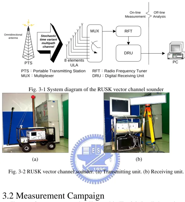
For measurement of the time-varying and directional mobile radio channels, the RUSK vector channel sounder was employed [9]. The measurement equipment and its system diagram and are shown in Fig 3-1 and Fig 3-2. The sounder system consists of a mobile transmitter (Tx) that is omni-directional, and a fixed receiver (Rx) with an 8-element array antenna, each having a beamwidth of 120 . A fast 0
multiplexing system switches between each of these elements in turn in order to take a complete vector snapshot of the channel in 12t . Periodic multi-frequency p
Doppler bandwidth of up to 20kHz allows complete statistical analysis of the time varying radio channel with respect to different azimuthally directions of the impinging waves. In the case of a remote link measurement, Tx/Rx synchronization is maintained by two rubidium references. This calibration process of rubidium reference removes the tracking error of the measurement system and as a result of phase and delay normalization. Allowing the system a warm-up time about 60 minutes to stabilize oscillator and amplifier minimizes temporal drift of the measurement system. The telemetry allows remote control of the digital receiving unit (DRU) from portable transmitting station (PTS) location.
The channel impulse responses of the antenna array are recorded as vector snapshots in rapid succession. After receiving by Rx, signals are gathered to DRU and sent to a personal computer (PC) to analyze where AOA is estimated by using Unitary ESPRIT with sub-array smoothing technology. An overview about array signal processing including estimation of the AOA and a comparison of ESPRIT with other algorithm can be found in [10]. The receiving antenna was mounted on a rooftop at 2.44 GHz with the transmission power of 1w. The transmitter antenna was carried in a trolley and was 1.8 meter above the road. In order to get multipath components, we sampled data by moving measurements along selected routes with walking speed. We performed the measurements at the time of 10:00~20:00 with many pedestrians and vehicles, which may result in random scattering effects.
RFT DRU MUX 8 elements ULA Omnidirectional antenna Stochastic time variant multipath channel
PTS Portable Transmitting Station MUX Multiplexer
Off-line Analysis On-line
Measurement
RFT Radio Frequency Tuner DRU Digital Receiving Unit
PC PTS
Fig. 3-1 System diagram of the RUSK vector channel sounder
(a) (b)
Fig. 3-2 RUSK vector channel sounder. (a) Transmitting unit. (b) Receiving unit.
3.2 Measurement Campaign
There are four measurement sites illustrated in Fig. 3-3. Detailed experimental setup or arrangement at each site is given as follows:
Measurement sites National Chiao Tung University Guang Fu campus Site 1 along route no.1 with total route length: 50m (12700 snapshots)
Site 2 along route no.2 with total route length: 170m (36700 snapshots)
Site 3 along route no.3 with total route length: 200m (4200 snapshots,)
Site4 along route no.4 with total route length: 250m (4800
snapshots) Moving speed
route no.1 and route no.2 : Speed=2~3 km/hr route no.3 and route no.4 : Speed=10 km/hr
Tx-Rx distance route no.1 15~50m route no.2 140m~150m route no.3 193~203m route no.4 250~259m
Transmit antenna Omni-directional
Height 1.8m Center frequency 2.44GHz Bandwidth: 120MHz
Transmit power 30 dBm Receive antenna 8-element ULA
Element spacing=0.5wavelength Bandwidth 120MHz
Time resolution 8.3ns Antenna effective height route no.1 1.8 m
route no.2 28.8 m
route no.3 and route no.4 21.6m Propagation delay time 1.6 s for route no.1.
6.4 s for route no.2, route no.3 and route no.4
We name site-ij as the particular propagation condition i along the measurement distance in route -j i.e., site12 means the LOS condition along route no.2, site23 means the OLOS condition along route no.3, site34 means the NLOS condition along route no.4
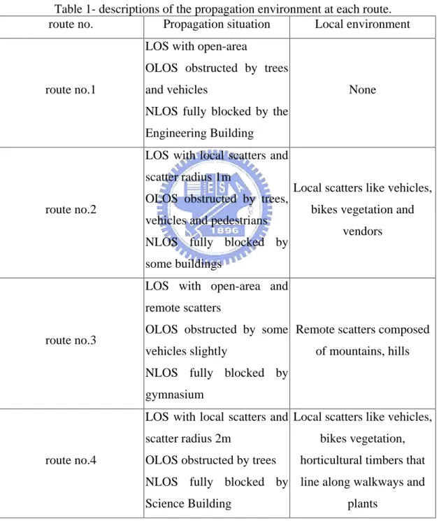
The propagation environment at each site is described as the following table.
Table 1- descriptions of the propagation environment at each route. route no. Propagation situation Local environment
route no.1
LOS with open-area
OLOS obstructed by trees and vehicles
NLOS fully blocked by the Engineering Building
None
route no.2
LOS with local scatters and scatter radius 1m
OLOS obstructed by trees, vehicles and pedestrians NLOS fully blocked by some buildings
Local scatters like vehicles, bikes vegetation and
vendors
route no.3
LOS with open-area and remote scatters
OLOS obstructed by some vehicles slightly
NLOS fully blocked by gymnasium
Remote scatters composed of mountains, hills
route no.4
LOS with local scatters and scatter radius 2m
OLOS obstructed by trees NLOS fully blocked by Science Building
Local scatters like vehicles, bikes vegetation, horticultural timbers that line along walkways and
Fig. 3-3 Measurement sites in the NCTU campus
MIMO channels can be modelled either as double directional channels or as vector (matrix) channels. The former method is more related to the physical propagation effects, while the latter is more emphasized on the effect of the channel on the system. Another distinction is whether to treat the channel deterministically or stochastically. In the following, we outline the relations between those description methods.
The deterministic double directional channel is characterized by its double directional impulse response. It consists of L propagation paths between the transmitter and receiver sites. Each path is delayed in accordance to its excess-delay
i, weighted with the proper complex amplitude
i
j i
a e and each direction of departure (AOD) T i, associated with the corresponding direction of arrival (AOA)
,
R i. The channel impulse response matrix h is
, , ( , , , ) ( , , , ) l ( ) ( ) ( ) L L j T R l T R l l T l R l l l h t h t e (10)
absolute time t; also the set of multipath components (MPCs) contributing to the propagation will vary, N N(t). The variations with time can occur both because of movements of scatters, and movement of the transmitter. The number of paths L can become very large if all possible paths are taken into account. In our experiments, the total number of resolvable multipath components was between 193 and 769. We simulate the deterministic channel applying the site-specific method to describe the direct wave, specular reflection waves, and single and multiple-over-rooftop diffracted waves. Once the site-specific method, i.e. deterministic method, is finished, the field strength distribution, power delay profile and power azimuth profile are shown in Fig. 3-4, we survey the multipaths in propagation, only one path is single rooftop diffracted wave accompanied with other 31 corner diffracted multipaths and acquire different realizations of the channel and proceed this procedure 15 times to obtain the complete channel matrix H4 4. Based on the theory of reciprocity of antenna, we obtain AOD by interchanging the position the transmitter and receiver. AOA T , AOD R in route no.1 case is approximately 0 . Repeating the 0 procedure above for 100 times gives an ensemble of channel realization and computes the capacity and plots a cumulative distribution function (CDF) for the MIMO channel capacity. Fig.3-4 gives the power delay profile and power azimuth profile of measurement for LOS of route no.1 and Fig 3-5 gives the time averaged Delay-Azimuth Spectrum of measurement of route no.1.
Fig 3-4. The field strength distribution of propagation, power delay profile and power azimuth profile for LOS of route no.1 in the left straight side, the ones which
Fig 3-6 (a)
Fig 3-6 (b)
Fig 3-6 (a) Field strength distribution of route no.2 and the Power Delay Profile and Power Azimuth Profile of route no.2 (b) Time Averaged Delay-Azimuth Spectrum of
Fig 3-7 (a)
Fig 3-7 (b)
Fig 3-7 (a) Field strength distribution of route no.3 and the Power Delay Profile and Power Azimuth Profile of route no.3 (b) Time Averaged Delay-Azimuth Spectrum of
Fig 3-8 (a)
Fig 3-8 (b)
Fig 3-8 (a) Field strength distribution of route no.4 and the Power Delay Profile and Power Azimuth Profile of route no.4 (b) Time Averaged Delay-Azimuth Spectrum of
3.3 Measurement data extraction
By examining the measurement raw data, we extracted the angle-of-arrival (AOAs), angle-of-departure (AODs), delays and azimuths of the multipath components [10].
Using the commercial software Matsys to obtain
(1) Time-variant Impulse Response h t( , , )s , where t represents observation time,
represents delay time, s represent channel, we take this to evaluate whether the environment is clean i.e. observing the Power Delay Profile had a trend of decaying along the propagation distance as time is going. In Fig. 3-9, we observe that (a)~(c) power level increases as time goes by and (c) appear apparent decaying situation at some measurement, the same bandwidth. In Fig. 3-9 (c), there is a time difference between the strongest receive signal power and next strong one around 0.25~0.3us, i.e. the multipath propagate to arrival receive array more over 75~90m. From these Power Delay Profiles, we recognize (a)~(c) as OLOS, NLOS and LOS, respectively and take these snapshots for data processing.
Fig. 3-9 The impulse response of (a) top (b) bottom left (c) bottom right figure presents the measurement during different observation time
(2) Delay-Azimuth spectrum extract multipath amplitudes from various azimuths and delays. We used Unitary ESPRIT (a parametric subspace estimation method incorporating forward-backward averaging) algorithm for detecting the information of direction to obtain time-variant delay-azimuth spread ht, , ( , , )t . There are two
kind of sampling result
Spatial sampling-for fixed (delay), extract multipath from various azimuths
Temporal sampling-for fixed (azimuth), extract multipath from various delay bins. From these two processing, we are ready to compute the effective multipath number under some environment and root mean square delay spread and azimuth spread, which can be used to evaluate the dispersionness of propagation.
Delay spread ( )= 2 2 ( ) ( ) ( ) ( ) ( ) k k k k k k k k k k P P P P Azimuth spread ( )= 2 2 ( ) ( ) ( ) ( ) ( ) k k k k k k k k k k P P P P
(3)Frequency response H(t, f, s) to obtain the corresponding MIMO capacity.
According to the propagation delay time and measurement bandwidth, we obtain 193 (or 769) delay bins in the Power Delay Profile and 193 (or 769) multipaths in the time domain contribute to the capacity through the Fourier transform in the frequency domain illustrated in Fig. 3-10. From consecutive snapshots received by array, we take a bundle of snapshots, depends on the element spacing, total measurement distance and moving speed, for representing the signal bursted out from one transmit antenna. Take the data of route no.1 10 element spacing at the transmit end for example, we need 312 snapshots to simulate the one transmit antenna, other three transmitter done in the same way. While the frequency responses from four transmitters are produced and averaged, we obtain a transfer channel matrix H4 4 193x x
(or H4 4 769x x ) and normalize to 2
,
1
ij i j
h , the normalization of channel matrix is in order to remove the path loss, the superscript of 193 (or 769) represents the frequency bins resolved from bandwidth and then compute the capacity of each frequency bin based on (5). This concept is merely like the expression below
( 6 0 ) ( 6 0 ) ( 6 0 ) ( 6 0 ) 1 1 1 2 1 3 1 4 ( 6 0 ) ( 6 0 ) ( 6 0 ) ( 6 0 ) ( 6 0 ) 2 1 2 2 2 3 2 4 ( 6 0 4 4 ( 6 0 ) ( 6 0 ) ( 6 0 ) ( 6 0 ) 4 4 3 1 3 2 3 3 3 4 ( 6 0 ) ( 6 0 ) ( 6 0 ) ( 6 0 ) 4 1 4 2 4 3 4 4 [ ] M H Z M H Z M H Z M H Z M H Z M H Z M H Z M H Z M H z x M H Z M H Z M H Z M H Z x M H Z M H Z M H Z M H Z h h h h h h h h H C h h h h h h h h )
M H Z ( 0 ) ( 0 ) ( 0 ) ( 0 ) 1 1 1 2 1 3 1 4 ( 0 ) ( 0 ) ( 0 ) ( 0 ) ( 0 ) 2 1 2 2 2 3 2 4 ( 0 4 4 ( 0 ) ( 0 ) ( 0 ) ( 0 ) 4 4 3 1 3 2 3 3 3 4 ( 0 ) ( 0 ) ( 0 ) ( 0 ) 4 1 4 2 4 3 4 4 [ ] M H z M H z M H z M H z M H z M H z M H z M H z M H z M x M H z M H z M H z M H z x M H z M H z M H z M H z h h h h h h h h H C h h h h h h h h )
H z ( 6 0 ) ( 6 0 ) ( 6 0 ) ( 6 0 ) 1 1 1 2 1 3 1 4 ( 6 0 ) ( 6 0 ) ( 6 0 ) ( 6 0 ) ( 6 0 ) 2 1 2 2 2 3 2 4 ( 6 0 ) 4 4 ( 6 0 ) ( 6 0 ) ( 6 0 ) ( 6 0 ) 4 4 3 1 3 2 3 3 3 4 ( 6 0 ) ( 6 0 ) ( 6 0 ) ( 6 0 ) 4 1 4 2 4 3 4 4
[
]
M H Z M H Z M H Z M H Z M H Z M H Z M H Z M H Z M H z M H z x M H Z M H Z M H Z M H Z x M H Z M H Z M H Z M H Zh
h
h
h
h
h
h
h
H
C
h
h
h
h
h
h
h
h
We view the capacity of different frequency bins sas the contribution of multipath and average it to obtain the corresponding array capacity for a sampled measurement.
Fig 3-10 (a) Fig 3-10 (b)
The procedures of Unitary ESPRIT to obtain AOA and AOD listed as below [11] 1. Initialization Form the matrix X CM N D from the available measurement
M represents an M-element sensor array composed of m pairs of pair-wise identical, but displaced sensors (doublets), i.e. M=4, N represent the number of selected snapshots, i.e. N=10, D represents the number of delay bins, i.e. D=193. 2. Signal Subspace Estimation Determine the real matrix T{ }X M 2N D
1 2 1 2 1 2 1 2 Re{G + G } Im{G G } T{ }=[ 2 Re{ } 2 Im{ } ] Im{G G } Re{G G } T T X g g
and compute the SVD of T{ }X (square root approach) or the eigendecomposition of T{ }X T{ }X H (covariance approach). The d dominant left singular vectors or eigenvectors will be called Es M d D. Estimate the number of sources d, if d is not a priori.
We consider an efficient computation of a particular transformation T ( ). It transforms an arbitrary complex matrix Cp q into a real p x 2q matrix, denoted by T (X). The block matrices G 1 and G2 should have the same size, we set them as
2 5 1 and G2
x
G C , 2 represent the 2 x 2 exchange matrix with ones on its antidiagonal and zeros elsewhere, i.e. 2 [0 1]
1 0 , 0
T
g since M is even. Then an efficient computation of T{ }X M 2N D from the matrix X only requires p x 2q real additions. Notice that d N.
3. (Total) Least Squares Solve the overdetermined system of equations
1 1 1 2 1 1 ( ) ( ) H m m M M H m m M M Q J J Q Q j J J Q where 2 2n+1 0 1 1 [ ] and Q [0 2 0 ] 2 2 0 n n n n T T n n n n n I jI I jI Q j j
we choose the size of subarray as 3, i.e. m=3, Q3 is the unitary matrix, J1 is the
selection matrix given by 3
1 0 1 [0 2 0 ] 2 1 0 j Q j , 1 1 0 0 0 [0 1 0 0] 0 0 1 0 J and, 4 1 0 0 0 1 0 1
Q [ ] 0 1 0 2 1 0 0 j j j j
, then we will obtain
1 2
1 1 0 0 0 0 1 1
[ 0 2 0 0 ] a n d [ 0 0 0 2 ]
0 0 1 1 1 1 0 0
4. Eigenvalue decomposition Compute the eigenvalue decomposition of resulting solution 1 d d T T
d k k=1
where =diag{w } eigenvalue matrix and exp( 0 t sin( ))
k k
w d w j
c
Chapter 4 Impact of propagation on capacity
Chapter 4
Propagation and Antenna Arrangement
Effects on MIMO Capacity
4.1 Propagation effect
Propagation at different conditions such as LOS, OLOS and NLOS may influence MIMO capacity. Here, we analyze the measured result along each route to see how the capacity changes as the conditions, propagation distance or local scatterer distribution varies, which is shown in section 4.1.1. Comparison between the measured result and the computed results from the ray-tracing based hybrid model will help to investigate the coupling effect between the element spacing and local scattering on the MIMO capacity. This is illustrated in section 4.1.2.
4.1.1 Measured result analysis
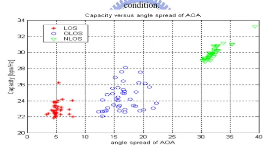
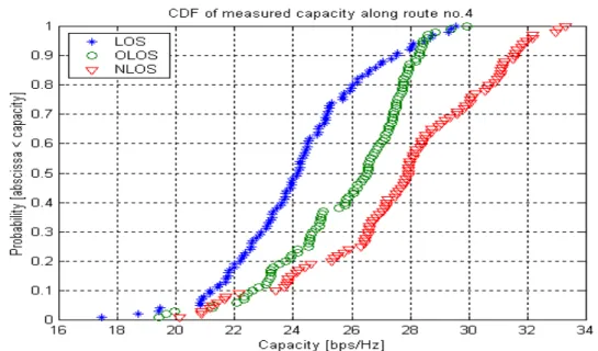
Figure 4-1 illustrates three CDFs of the measured MIMO capacity for LOS, OLOS and NLOS conditions along route no.1. There are three CDF curves to show the results of LOS, OLOS and NLOS conditions. The averaged capacity is 13.1102 bps/Hz for LOS condition, 14.9382 bps/Hz for OLOS condition and 15.65 bps/Hz for NLOS condition. It is found that the capacity in the LOS condition is smaller than that of the OLOS or NLOS condition. It is because that the rms AOA angular spread of the LOS condition is smaller than that of latter two conditions. The larger multipath angular dispersion will lead to less spatial correlation between receiving signals, i.e., larger capacity. This result is shown in Figure 4-2 where larger rms angle spread leads
capacity of LOS, OLOS and NLOS conditions, respectively. Similar results are found in the figure 4-4 for route no.2, figure 4-5 for route no.3 and figure 4-6 for route no.4.
Fig 4-1 The CDF of the measured MIMO capacity for LOS (*), OLOS (o) and NLOS ( ) conditions along route no.1. The averaged capacity is 13.1102 bps/Hz for LOS
condition, 14.9382 bps/Hz for OLOS condition and 15.65 bps/Hz for NLOS condition.
Fig 4-2 capacity versus rms angular spread of AOA for LOS (*), OLOS (o) and NLOS ( ) conditions
11 12 13 14 15 16 17 0 5 10 15 Capacity [bps/Hz] P ro b a b ili ty d e n s it y
4x4 for MIMO outdoor along LOS of route no.1
LOS
Fig 4-3 (a) 10 11 12 13 14 15 16 17 18 19 0 2 4 6 8 10 12 14 16 P ro b a b ili ty d e n s it y
4x4 for MIMO outdoor along OLOS of route no.1
OLOS
12 13 14 15 16 17 18 19 20 21 22 0 2 4 6 8 10 12 Capac ity [bps /Hz ] P ro b a b ili ty d e n s it y
4x 4 for M IM O outdoor along NLOS of route no.1
NLOS
Fig 4-3 (c)
Figure 4-3 The histogram of MIMO capacity for (a) LOS, (b) OLOS and (c) NLOS conditions.
Fig 4-4 The CDF of the measured MIMO capacity for LOS (*), OLOS (o) and NLOS ( ) conditions along route no.2. The averaged capacity is 23.258 bps/Hz for LOS
condition, 24.623 bps/Hz for OLOS condition and 24.8787 bps/Hz for NLOS condition.
Fig 4-5 The CDF of the measured MIMO capacity for LOS (*), OLOS (o) and NLOS ( ) conditions along route no.3. The averaged capacity is 21.7373 bps/Hz for LOS
condition, 23.8253 bps/Hz for OLOS condition and 25.732 bps/Hz for NLOS condition.
Fig 4-6 The CDF of the measured MIMO capacity for LOS (*), OLOS (o) and NLOS ( ) conditions along route no.4. The averaged capacity is 24.1806 bps/Hz for LOS
condition, 25.8532 bps/Hz for OLOS condition and 27.6917 bps/Hz for NLOS condition.
4.1.2 Comparison among different routes
Fig 4-7 (a)~(c) illustrates the CDF of capacity of different routes for LOS, OLOS and NLOS respectively. From these three figures, we can obtain that the capacity performance of route no.1 is always smaller than that of others despite the LOS, OLOS and NLOS conditions. The performance of MIMO capacity along route no.2, route no.3 and route no.4 has some degree of resemblance. Since the distinctions of the measurement in the route no.1 with that of other three are the propagation distance and local scatterers, so we sample the capacity from measurement along the propagation distance for each route shown as Fig 4-8 and apply hybrid model shown as Fig 4-9 to investigate the effect of propagation distance on the capacity performance. In the same way, we compare Fig 4-10 with the figure applying hybrid model shown as Fig 4-11 for each route to investigate the effect of local scatterers on the capacity performance.
Fig 4-7 (b)
Fig 4-7 (c)
Fig. 4-7 (a) The CDF of capacity of LOS in each route, (b) the CDF of capacity of OLOS in each site and (c) the CDF of capacity of NLOS in each site. There are four CDF curves to show the results of LOS condition of route no.1, route no.2, route no.3 and route no.4 in Fig 4-7 (a), four CDF curves to show the results of OLOS condition of route no.1, route no.2, route no.3 and route no.4 in Fig 4-7 (b) and four CDF curves
to show the results of NLOS condition of route no.1, route no.2, route no.3 and route no.4 in Fig 4-7 (c).
Fig 4-8 obviously presents that the capacity performance of shorter propagation distance 50m is indeed inferior to the one of other longer propagation distance. It despitse that propagation distance effect at each route does not exhibit regular trend and larger capacity deviation. Another information given by Fig 4-8 is that the standard deviation of capacity of propagation distance 50m is the smallest among the measurement results. This phenomenon tells us that transmitted signals through longer propagation distance may experience more complex channel so that causing more multipaths in the channel. In this way, the transmitted signals received by the opposite array will be less correlated each other, resulting in larger capacity fluctuation. Fig 4-9 shows that the computed results of CDF of the measurement along propagation distance. All are resembled except one in asterisk line sampled from route no.1 along propagation distance 50m.
Fig 4-10 shows the capacity variation of the LOS condition of measurements in all routes. It also provides us with the information of standard deviation of capacity sampled from all measurements, although the standard deviation of capacity in route no.1 is almost equal to the one in route no.3, the averaged capacity of measurements along route no.1 is much smaller than that of measurements along route no.3. This phenomenon can be explained as that the LOS condition around the route no.1 belongs to open-area and short distance, while the LOS condition around route no.3 characterized by distant scatters backed up with hills so that the transmitted signal propagated within quite small rms angular spread of AOA to the receive array. Otherwise, in the cases of route no.2 and route no.4, the capacity fluctuation differs from that of route no.1 and route no.3 significantly. Since the local scatterers like vehicles and pedestrians surrounded the transmitter in the LOS of route no.2 and route no.4 so that the transmitted signals within an extremely large rms angular spread of
AOA propagated to the receive array, resulting in transmitted signals less correlated each other. That is why the standard deviations of capacity of route no.2 and route no.4 vary dramatically. Fig 4-11 shows the computed results of CDF of LOS with local scatters in all measurements plus the case of LOS in route no.1 without local scatterer. From figure 4-8 to 4-11, we conclude that the propagation distance and local scatterers around transmit end array will affect the capacity performance.
Fig 4-8 The capacity variation of different propagation distance D from measurement with standard deviation of the capacity C D, 50m 0.9568 bps/Hz, C D, 150m 1.3368 bps/Hz, C D, 200m 1.2761 bps/Hz, C D, 250m 1.8584bps/Hz and C D, 300m 2.5649
Fig 4-9 The CDF of capacity for different propagation distance applying hybrid model
Fig 4-10 The capacity variation of LOS along different routes with standard deviation of capacity C route no, .1 0.718 bps/Hz, C route no, .2 1.3745 bps/Hz, C route, no.3 0.7187
Fig 4-11 The computed CDF of the MIMO capacity for routes no.1-4 by using the hybrid model.
Fig 4-12 shows the averaged capacity of each route. It is found that in every route the capacity of LOS condition is always smaller than that of the OLOS or NLOS condition. It is because that the existence of direct path will reduce the rank of the channel matrix, which becomes a dominant factor in reducing the MIMO capacity.
4.2 Element spacing effect
In this section, we investigate the impact of MIMO element spacing on capacity through the measured data. Comparison between the measurement result and the computed results using the ray-tracing based hybrid model will help to investigate the coupling effects between the element spacing and local scatterers on the MIMO capacity. Section 4.2.1 will introduce the measurement of MIMO element spacing for LOS, OLOS and NLOS conditions. Section 4.2.2 provides the computation results using the hybrid model. Section 4.2.3 compares the measurement and computed MIMO capacity.
4.2.1 Measurement Result Analysis
Fig 4-14 gives the capacity variation under LOS with MIMO element spacing for route no.1 and Fig 4-15 corresponding CDF of different element spacing. Figure 4-14 indicates that the capacity increases as the element spacing increases. Since the element spacing increases, the array aperture is approximately M x d , beamwidth is t
inversely proportional to aperture and resolution is inversely proportional to beamwidth, hence the larger array ( dt larger) resolves multipaths more, the propagation of MIMO channel filled with multipaths lead to the capacity to increases. Figures 4-16 (a), (b) and (c) demonstrates the histograms of MIMO capacity with element spacing 10 ~ 30 along route no.1, respectively. Similar results are found in the figure 4-17 (a) for route no.2, figure 4-17 (b) for route no.3 and figure 4-17 (c) for route no.4.
Fig 4-14 The capacity variation under LOS with MIMO element spacing for route no.1 with standard deviation of capacity C, 10 0.7009 bps/Hz, C, 20 1.1148
bps/Hz and C, 30 0.7592 bps/Hz
Fig 4-15 The CDF of different element spacing for LOS along route no.1. The averaged capacity is 13.1102 bps/Hz for 10 condition, 14.0516 bps/Hz for
Fig 4-16 (a)
Fig 4-16 (c)
Fig 4-16 histogram corresponding to MIMO capacity for LOS along route no.1 with (a) 10 (b) 20
(c) 30
Fig 4-17 (a) The CDF of different element spacing for LOS along route no.2. The averaged capacity is 23.258 bps/Hz for 10 condition, 23.6484 bps/Hz for
Fig 4-17 (b) The CDF of different element spacing for LOS along route no.3. The averaged capacity is 21.7373 bps/Hz for 10 condition, 22.4905 bps/Hz for
20 condition and 24.0012 bps/Hz for 30 condition.
Fig 4-17 (c) The CDF of different element spacing for LOS along route no.4. The averaged capacity is 24.2358 bps/Hz for 10 condition, 25.83 bps/Hz for
20 condition and 26.3559 bps/Hz for 30 condition.
Fig 4-18 illustrates the ensemble average capacity with MIMO element spacing of measurements. As the figure indicated, there will be a trend that capacity becomes
large as the MIMO element spacing increases for each route. Note that the values shown in the Fig 4-18 are obtained from averaging statistically 100 times.
Fig 4-18 The averaged capacity with MIMO element spacing for all measurements
4.2.2 Computation with the Hybrid model
From [12], a hybrid spatio-temporal radio channel model combines a site-specific model with a statistical model; we simulate the MIMO propagation with different element spacing and local scatters around the transmitter, in the process of adding the local scatters to investigate effect on MIMO capacity, there are three categories of local scatters effect, they are the category of 3 local scatters and scatter radius 2m with 4 different transmit element spacing 10 , 20 , 30 , shown in Fig 4-19 (a); the category of scatter radius 2m and transmit element spacing 10 with 2 to 6 local scatters, shown in Fig 4-19 (b); the category of 3 local scatters and transmit element spacing 10 with 3 different scatter radius 2m, 3m, 4m, shown in Fig 4-19 (c). In Fig. 4-19 (a), we note that the ensemble capacity will increase as the element spacing increases since the array aperture is approximately M x d , beamwidth is
inversely proportional to aperture and resolution is inversely proportional to beamwidth, hence the larger array ( d larger) resolves multipaths more, the t
propagation of MIMO channel filled with multipaths results in capacity increases. Fig 4-19 (b) and (c) present the degree of freedom of local scatter and scatter radius essentially perturb the MIMO channel and decorrelate it such that capacity distributes wider. This says the scatters within scatter radius around the transmitter will have impact on the MIMO capacity with 13.35% variation.
Fig 4-19 (a)