國立交通大學
統計學研究所
碩 士 論 文
利用OAAT方法監控第一階段非線性剖面資料之研究
The OAAT Scheme for Phase I Nonlinear Profile Monitoring
研 究 生:許怡玲
指導教授:洪志真 博士
研 究 生:許怡玲 Student: Yi-Ling Hsu
指導教授:洪志真 博士 Advisor: Dr. Jyh-Jen Horng Shiau
國立交通大學
統計學研究所
碩士論文
A Thesis
Submitted to Institute of Statistics College of Science
National Chiao Tung University in Partial Fulfillment of the Requirements
for the Degree of Master
in Statistics June 2006
Hsinchu, Taiwan, Republic of China
研究生:許怡玲 指導教授:洪志真 博士
國立交通大學統計學研究所
摘 要
Shiau
和
Sun(2006) 針對第一階段製程監控提出OAAT法,即研究一次只
剔除一個最極端的管制外樣本點的作法。模擬研究顯示,「OAAT」法可大幅
降低假警報之發生,因此,我們將此方法推廣到剖面資料的監控。本文使用
一個建構於加權最小橢球體積
(
Reweighted Minimum Volume Ellipsoid)估計量之 T
2控制圖來監控剖面資料。我們比較OAAT法和傳統的方法(每次管制界限外的樣
本點全部刪除)的假警報率(製程在穩定狀態,但監控統計量落在管制界限建
以外的比例)和偵測力(製程發生改變,而監控統計量落在管制界限以外)
。我
們證明OAAT法可以降低製程監控的假警報,而且研究結果也發現當製程偏移
的夠大和管制界限是單邊的時候,這兩個方法的假警報是非常接近的。因為
傳統的方法在計算上是較經濟的,所以我們提出一個統計量當準則去決定何
時使用哪個方法,可使製程監控更精確更有效率。最後,我們利用兩個真實
資料去證明我們所提出的理論方法。
Student:Yi-Ling Hsu Advisors:Dr. Jyh-Jen Horng Shiau
Institute of Statistic
National Chiao Tung University
Abstract
Shiau and Sun (2006) proposed an one-at-a-time (OAAT) scheme for Phase I process monitoring that only discards the most extreme out-of-control sample at a time. Using Shewhart
X chart as an example, they demonstrated that the OAAT scheme reduces dramatically the occurrences of false alarms. In this paper, we extend this scheme to nonlinear profile monitoring. We consider a T2 chart constructed based on the reweighted minimum volume ellipsoid (RMVE) for profile monitoring. We compare the false-alarm rate (the possibility that an in-control sample is claimed as out of control) and detecting power (an out-of-control sample is detected) of the OAAT scheme with that of the traditional delete-all scheme and confirm that the OAAT scheme reduces the false-alarm rates while attaining the detecting power in profile monitoring. It is also found that when the process shift is large enough, the false-alarm rates of the two schemes are very close for one-sided control charts. Since the Delete-All scheme is more economic in computation, we provide a statistic as a guide on when to use it for achieving the efficiency. Finally, we demonstrate the methodologies described in the thesis with two real-life examples.
誌 謝 辭
這篇論文的完成,最要謝謝洪志真教授一年來不倦不悔的指導跟辛苦的批閱和指導, 在老師的指點之下,讓我逐漸能將統計應用於生活上,並且引導我學習與研究的方向。除 了課業上的知識以外,老師也讓我學到許多求知與做研究的方法,讓我在工業統計這片領 域中,找到我的興趣跟做出研究的成就感。還要感謝博班家鈴學姐的大力幫助,春火學長 的有效的教導,和香菱和筱娟同學給予我鼓勵,除了課業上的切磋討論外,閒暇之餘能跟 他們閒話家常,交換各種意見與心得,讓我的生活充滿樂趣,在互相鼓勵之下度過研究所 的生涯,還有感謝郃嵐、珮琦、佩蓁、瑜達和政言,有他們我才有能力順利完成學業。另 外也感謝所上每位老師在授課所以給予的觀念,讓我受益良多。加上心愛的家人-爸爸、媽 媽、小薇、小藍、唐霖的支持與關懷,讓我非常順利的完成論文。 同時感謝口試委員黃榮臣教授、曾勝滄教授和陳鄰安教授提供諸多建議,使得本論文 更加完善。 剛開始抱著期待與學習的心來到交大統研,系上提供良好的學習環境。現在,我將懷 著感謝與難忘的心情離開,在這充滿了班上同學跟老師的回憶,包含了迎新、家聚和送舊 等等。我很開心自己是交大統研所的一員,未來也會努力工作為所上爭光。 最後,僅將論文獻給敬愛的父母親和洪志真教授,感謝他們的辛勞,我愛他們,就因 為有他們,才有現在信心滿滿,不怕未來挑戰的我。所有在我周圍關心我的人,一同分享 此篇論文完成之喜悅與榮耀,謝謝大家。 許怡玲 謹 誌于 國立交通大學統計研究所 中華民國九十七年六月英文摘要... ii
誌 謝 辭... iii
Contents... iv
List of Table... vi
List of Figure... vii
1. Introduction... 1
2. Literature Review... 5
2.1 Profile Monitoring ... 5
2.1.1 Linear Profiles ... 5
2.1.2 Nonlinear Profiles... 6
2.2 Minimum Volume Ellipsoid (MVE)... 9
3. A Study of the One-At-A-Time Scheme in Profile Monitoring Scheme ... 12
3.1 Motivation ... 12
3.2 The OAAT Scheme... 12
3.3 Simulation Studies... 12
3.3.1 Simulation settings ... 13
3.3.2 Results of Simulation Studies... 13
4. A Guideline for which Scheme to Use ... 19
4.1 Estimate the Real Variance from the Truncated Data... 19
4.2 The statistic for univariate data ... 21
4.3. Simulation for univariate data ... 25
4.4 The Statistic for Multivariate Data ... 26
4.5 Simulation for multivariate data... 28
5. Examples... 30
5.2 Vertical Board Density Data (VDP)... 41
5.2.1 Data Description... 41
5.2.2 Monitoring the VDP Data... 44
5.3 The
T
02 Statistic for Examples ... 456. Conclusion... 46
References... 47
Appendix A... 49
A.1. Truncated Normal Distribution... 49
A.2. Truncated Multivariate Normal Distribution... 51
Table 1: The value of C for bias correction of the variance estimated by the truncated normal data for various α (p=1)... 20 Table 2: The value of C for bias correction of the variance estimated by the truncated normal
data for various α (p=2)... 20 Table 3: The value of C for bias correction of the variance estimated by the truncated normal
data for various α (p=4)... 21
Table B. 1: The control limit for 2 RMVE
Figure 2: The triangle points are out of control, the solid ellipsoid is based on the RMVE
estimator...11 Figure 3: Comparisons of the OAAT scheme and Delete-All scheme for m1=3, m=25, and p=2 in
terms of (a) the false-alarm rate, and (b) the detecting power. ... 14 Figure 4: Comparisons of the OAAT scheme and Delete-All scheme for m1=3, m=25, and p=4 in
terms of (a) the false-alarm rate, and (b) the detecting power. ... 14 Figure 5: An example with shift size |δ|=5... 15 Figure 6: An example with shift size |δ|=10... 15 Figure 7: Effects of p on the OAAT scheme (a) The false-alarm rate, and (b) the detecting power
for m1=3, m=25, and p=2, 4. ... 16 Figure 8: Effects of p on the Delete-All scheme (a) The false-alarm rate, and (b) the detecting
power for m1=3, m=25, and p=2, 4. ... 16 Figure 9: Effects of m on the OAAT scheme. (a) The false-alarm rate, and (b) the detecting power for m=25(25)100, m1=3(3)12, and p=2. ... 17 Figure 10: Effects of m of the Delete-All scheme. (a) The false-alarm rate, and (b) the detecting
power for m=25(25)100, m1=3(3)12, and p=2... 17 Figure 11: Effects of the proportion of out-of-control data on the OAAT scheme. (a) The
false-alarm rate, and (b) the detecting power for m1=3(3)12, m=50, and p=2. ... 18 Figure 12: Effects of the proportion of out-of-control data on the Delete-All scheme. (a) The
false-alarm rate, and (b) the detecting power for m1=3(3)12, m=50, and p=2. ... 18 Figure 13: Truncated normal distribution with 50% truncated (α=0.5). (a) p=1 and (b) p=2. .... 21
Figure 14: The density plot of 100,000 simulated T0 values. (a) The density plot, and (b) the histogram plot. ... 22 Figure 15: The normal Q-Q plot for 100000 simulated statistic T0 ... 22 Figure 16: Detect univariate data by X chart (two-tailed). (a) The false-alarm rate, and (b) the
The false-alarm rate, and (b) the detecting power... 23
Figure 18: Detect univariate data by S chart and the subgroup is greater than 6 (two-tailed). (a) The false-alarm rate, and (b) the detecting power... 24
Figure 19: R chart (one-tailed). (a) The false-alarm rate, and (b) the detecting power... 24
Figure 20: R chart (one-tailed). (a) The false-alarm rate, and (b) the detecting power... 25
Figure 21: An example for X chart. (a) 10 times shift, and (b) no shift... 25
Figure 22: T0 for simulated univariate data. (a) R chart, and (b) S chart (one-tailed test). ... 26
Figure 23: The plot of the statistic 2 0 T from simulated multivariate data. (a) The density plot, and (b) the histogram plot... 27
Figure 24: The chi-square Q-Q plot for the statistic 2 0 T from simulated multivariate data. ... 27
Figure 25: 2 0 T from simulated multivariate data for p=2 and p=4. ... 28
Figure 26: 2 0 T for simulated multivariate data. (a) p=2, and (b) p=4... 29
Figure 27: Bioassay Data (DuPont Does-Response Data) for all 44 weeks... 31
Figure 28: A does-response curve... 32
Figure 29 : Estimated mean profiles of all 44 weeks in the bioassay data ... 33
Figure 30: The RMVE chart when monitoring unusual profiles. (a) The 44 dose-response profiles at the first iteration, and (b) the 33 dose-response profiles at the last iteration. ... 34
Figure 31: Estimated variance profiles of all 44 weeks in the bioassay data. ... 36
Figure 32: The RMVE chart when monitoring the remaining variance profiles by the OAAT scheme. (a) The 44 variance profiles, and (b) the 42 variance profiles. ... 37
Figure 33: The RMVE chart when monitoring the remaining variance profiles by the Delete-All scheme. (a) The 44 initial variance profiles, (b) the 38 variance profiles, after the 1st iteration, and (c) the remaining 34 variance profiles. ... 38
Figure 34: The RMVE chart when monitoring the remaining mean profiles by the OAAT scheme. (a) The 42 mean profiles, (b) the 33 mean profiles... 39
profiles. ... 40
Figure 36: The thick lines are the 6th, 16th, 19th, and 44th profiles... 41
Figure 37: The 24 profiles in the VDP data... 42
Figure 38: Fittings of the 24 profiles in the VDP data. ... 43
Figure 39: The RMVE chart when monitor VDP profile. (a) The 24 boards at the first iteration, (b) the 22 boards at the 2nd iteration, and (c) the 18 boards at the final iteration. ... 44
1. Introduction
Control chart is a powerful tool in statistical process control (SPC) for achieving process stability and improving capability through the reduction of variability. The statistic used in constructing a control chart usually is a quality-related variable or a random vector consisting of several possibly correlated quality characteristics of a process or a product. However, in many practical situations, the quality of a process or a product is better characterized by a relationship between a response variable and one or more explanatory variables. Thus, for a sample, one observes a collection of data that can be represented by a curve (or profile). The profile can be linear or nonlinear. In this paper, we consider both casts of linear and nonlinear profile. Linear profiles are first fitted by a simple linear regression model and the estimated parameters are used for process monitoring. The monitoring of linear profiles can be applied to a wide variety of applications. In particular, most of studies in linear profile monitoring have been motivated by calibration applications. A nonlinear profile very often expressed as a high dimensional data vector. But most of multivariate data analysis technique will face the ill-condition problem due to the high correlation between data on the same profile. Because of this, we often use a Hotelling
T2 statistic of the estimated regression parameters to monitor profiles.
Process monitoring based on control charting usually consists of Phase I and Phase II. Control charts are used primarily in Phase I to bring the process to the in-control state. The purpose of this paper is to study the OAAT scheme proposed by Shiau and Sum (2006) for Phase I profile monitoring. A historical data set is collected and trial control limits are constructed to determine if the process is in-control. If so, then we have an in-control data set to establish adequate control limits for future on-line process monitoring.
In Phase I, to construct a control chart to monitor samples collected from the process, we use the samples to establish trial control limits for the monitoring statistic, such as Hotelling T2
statistics. For simplicity, if samples are outside the control limit, then we claim that the samples are out of control. If some samples are out of control, then the process may have assignable causes for these out-of-control samples. If some assignable causes are found, then these
out-of-control samples should be removed, otherwise, one needs to make a decision on eliminating these samples or not. No one knows which action is correct without further information since data points may exceed the limits simply by chance or due to be some uncovered assignable causes. For being conservative, many practitioners may choose to discard these potential〝out-of-control〞samples. After eliminating these out-of-control samples, the trial control limits need to be recalculated with the remaining samples to check if the data set still contains any out-of-control samples. The above screening steps are repeated until no more out-of-control samples are present. We then use the in-control process data attained in Phase I to estimate process parameters, e.g., the mean and standard deviation, of the monitoring statistic for setting up reliable control limits to monitor new process data in Phase II.
Statistically, there are possibilities that some in-control samples will be claimed concluded as out of control and some out-of-control samples as in control, which are similar to committing Type I and Type II errors in hypothesis testing, respectively. A good control chart should be able to control these two types of error rates. Because out-of-control samples usually make the trial control limits too wide, some out-of-control samples are not detected and removed. On the other hand, if some in-control samples are eliminated, some estimation efficiency is lost. Thus one would link to have effective procedure for collecting in-control data for Phase II usage. For more discussions regarding the differences between analyses of Phase I and Phase II, one is referred to Mahmoud and Woodall (2004) and Sullivan (2002). We focus on Phase I analysis in this paper.
Robust estimation methods are more effective in detecting unusual data points, and the control limits constructed with these robust estimates would be more reliable. But robust estimation for multivariate data or profiles are not as straightforward nor as easily implemented due to the extensive computation required to obtain the estimates.
Recently, some researches study robust estimation methods for detecting multivariate outliers. Outliers in multivariate data are more difficult to detect than that in univariate data. Woodruff and Rocke (1994) discussed some approaches, such as the minimum volume ellipsoid estimator (MVE) proposed initially by Rousseeuw (1984) and the minimum covariance determinant (MCD)
estimator proposed by Rousseeuw (1984) and Rousseuw and Van Deiessen (1999), are well suited for detecting multivariate outliers. These approaches can avoid “bad” data to “mask effects” in multivariate data. Shiau, Yen and Feng (2006) proposed using a Hotelling T2 chart based on MCD estimators in conjunction with the False Discovery Rate (FDR), and demonstrated that the chart is effective in detecting a reasonable number of outliers.
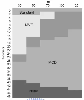
Jensen, Birch, and Woodall (2007) compared the standard, MVE and MCD estimator. Figure 1 (from Jensen et al. (2007)) shows that best estimator among the three for various sample sizes
m of the historical data set and percentage of outliers. They concluded that the MVE method is best for small values of m and proportion of outliers is small. We use two data sets for demonstration in this study, one is the bioassay data given in Williams, Woodall, Ferry, and Birch (2007) and the vertical board density profile (VDP) data set given in Walker and Wright (2000). The bioassay data set consists of 44 profiles and the VDP data consists of 24 profiles. Both examples have fewer than 50 samples. We adopt the MVE estimator in this study, since the number of profiles m is small in two examples.
Rousseeuw and Leroy (1987) divided the MVE into the MVE and the Reweight MVE (RMVE). The RMVE is more robust than MVE, because the RMVE estimator is not affected by outliers. In this paper, we use the RMVE estimator to monitor samples.
Figure 1: A summary of the preferred estimator for p=2. (from Jensen et al. (2007))
For detecting out-of-control profiles and preventing losing too many in-control profiles, Shiau and Sun (2006) proposed an iterative procedure called One-At-A-Time (OAAT) scheme that discards only the most extreme beyond-limits point and then updates the control limits at each iteration. We refer to the traditional scheme that deletes all of the out-of-control profiles at a time and claims that it is the〝Delete-All〞scheme. For comparing two schemes, we use the following two measures: (i) the false-alarm rate, defined as the probability that an in-control sample is claimed as out of control; and (ii) the detecting power, is the probability that an out-of-control sample is detected. For example, let m=25 and m1=3, where m is the number of profiles and m1 is the number of out-of-control profiles. If one in-control profile is claimed as an out-of-control profile, then the false alarm rate is 1/(25-3). If two out-of-control profiles gets detected, then the detecting power is 2/3.
In this paper, we use a robust Hotelling T2 statistic, to monitor profile data for Phase I analysis, and apply the OAAT scheme to the bioassay data given in Williams, Birch, Woodall,
and Ferry (2007) and to the VDP data given in Walker and Wright (2002). We compare the Delete-All scheme and the OAAT scheme in terms of the false-alarm rate and detecting power. We confirm that the OAAT scheme reduces the false-alarm rates while attaining the detecting power in profile monitoring. It is also found that when the process shift is large enough, the false-alarm rates of the two schemes are very close for one-sided control charts. Since the Delete-All scheme is more economic in computation, we provide a statistic as a guide on when to use it for achieving the efficiency.
Section 2 reviews linear/nonlinear profile monitoring, and robust multivariate control charts. Section 3 compares the OAAT scheme with the Delete-All scheme, and Section 4 give a guideline on which scheme to use for real data. Section 5 demonstrates our method with the bioassay data and the VDP data. Finally, we conclude the thesis in Section 6.
2. Literature Review
2.1 Profile Monitoring
2.1.1 Linear Profiles
There are some literatures on fixed-effect models. For example, Kang and Albin (2000) combined the EWMA chart with R chart (EWMA-R chart) for Phase II linear profile monitoring. Because the EWMA chart is not sensitive to shifts on the process variation and not sensitive to larger shifts on intercept and slope, Kim, Mahmoud, and Woodall (2003) provided a combined three EWMA chart for Phase II. It can detect shifts quicker than the EWMA-R chart in Kang and Albin (2000). Mahmoud and Woodall (2004) suggested an F-test approach using indicator (dummy) variables in a multiple regression model, and proposed the likelihood ratio test for detecting changes in one or more regression parameters.
There are some literatures on random-effect models. Assume that m profiles are available. For
the ith random sample collected over time, we have the observations (xi, yij), i = 1,2,…,m, and j =
1,2,…,n. For each sample, we assume that the linear regression model relating the independent
0 1 , 1,..., , 1, 2,..., , ij i i ij ij y = A +A x +ε i= m j= n (1) where . . . 2 . . . 2 . . . 2 0 ~ ( ,0 0) , 1 ~ ( ,1 1) , ~ (0, ) i i d i i d i i d i i ij i
A N α σ A N α σ ε N σ , and X values are fixed and take the
same set of values for each sample.
Shiau, Lin, and Chen (2006) proposed a linear profile monitoring scheme based on the above random-effect model to incorporate the subject-to-subject variation that exists in many real-life problems. Jensen, Birch, and Woodall (2006a) proposed a linear mixed model (LMM). The LMM is very flexible and capable of fitting a large variety of datasets and allows us to account for the correlation within profiles and to consider the profiles as random samples from a common population distribution, which may be more realistic in many applications.
There are more literatures on linear profile monitoring and its applications. For example, see Mestek, Pavlik, and Suchanek (1994), Stover and Brill (1998), Brill (2001), Jensen, Birch, and Woodall (2006a), and the references cited therein.
2.1.2 Nonlinear Profiles
Profiles that cannot be adequately represented by a linear model are generally referred to as nonlinear profiles. A common approach is to model the nonlinear profiles by a nonlinear parametric regression model. Taking the estimated parameter vector of the regression function as the representative of the profiles, monitoring nonlinear profiles can them be considered as a particular application of multivariate process control problems.
Shiau, Yen, and Feng (2006) proposed a Hotelling T2 chart based on the Minimum Covariance Determinant (MCD) estimators. And it is effective in detecting any reasonable number of outliers. Williams, Woodall, and Birch (2003) fitted a nonlinear regression to model the vertical density profiles (VDP) data, compared three T2 control charts (using sample covariance matrix, successive differences, and intra-profile pooling as estimates of the covariance matrix, respectively) to monitor the VDP data, and analyzed the advantages and the drawbacks of
the three control charts.
Jensen, Birch, and Woodall (2006b) proposed an approach to detect changes in Phase I, replacing the nonlinear model (NL model) by nonlinear mixed model (NLM model), such that the NLM approach has much higher probability of detecting the change than the NL approach.
Shiau, Lin, and Tsai (2006) used the technique of principal components analysis to analyze the covariance structure of the nonlinear profiles nonparametrically. Ding, Zeng, and Zhou (2006) proposed using independent components analysis in nonparametric procedures to Phase I analysis for multivariate nonlinear profiles. The authors mentioned that the high dimension of profile data and data contamination present a challenge to the Phase I analysis of nonlinear profiles. Such nonparametric models do not have a specific functional form and have no model parameters to estimate, but rather one employs smoothing techniques such as local polynomial regression or spline smoothing to model a profile.
Nonparametric regression techniques provide great flexibility in modeling the response. One disadvantage of nonparametric smoothing methods is that the subject-specific interpretation of the estimated nonparametric curve may be more difficult, and may not lead the user to discover assignable causes for an out-of-control signal as easily as parametric regression methods.In this study, we consider the parametric regression method.
There are more literatures on nonlinear profile monitoring and its applications, such as Williams, Birch, Woodall, and Ferry (2007) proposed nonlinear profile monitoring methods to monitor the variability of multiple assays.
Assume that we have m profiles of data and each profile contains n measurements. Let yij refer to the jth measurement of the ith profile. A nonlinear profile of an item can be modeled by the nonlinear (parametric) regression model given generally by
( , ) 1,..., , 1,..., ,
ij ij i ij
y = f x β +ε , i= m j= n (2)
where xij is the jth set point of the ith profile, . . . 2 ~ (0, ) i i d ij N i ε σ , βi is a p by 1 vector of parameters
for profiles i, and ( )f ⋅ is a function which is nonlinear in the parameter vector βi.
Because nonlinear parametric regression estimation is not as easy as linear regression estimation, we describe a method for nonlinear parametric regression estimation below. We rewrite the form in (3) by stacking the n observations within each profile into a vector as
1 2 ( , ,..., ) ' i = y yi i yin y , xi =( ,x xi1 i2,...,xin) ' , f( , ) ( ( , ), ( , ),..., ( , )) 'x βi i = f xi1 βi f xi2 βi f xin βi , and 1 2 ( , ,..., ) ' i = ε εi i εin
ε . The vector form of Equation (3) is then given by
( , ) 1,...,
i = f i i + i i= m
y x β ε , . (3)
For the nonlinear regression model given in (3), we first obtain the estimate of β for each i
profile. This is usually accomplished by employing the Gauss-Newton procedure and iteration to obtain the least squares estimates. Define the n by p matrix of the derivatives of ( , )f x β with i i
respect to β as i 1 1 1 1 2 2 2 2 1 2 1 2 ( , ) ( , ) ( , ) ( , ) ( , ) ( , ) ( , ) . ( , ) ( , ) ( , ) i i i i i i i i ip i i i i i i i i i i ip i i in i in i in i i i ip f x f x f x f x f x f x f F f x f x f x β β β β β β β β β ∂ ∂ ∂ ⎡ ⎤ ⎢ ∂ ∂ ∂ ⎥ ⎢ ⎥ ⎢∂ ∂ ∂ ⎥ ⎢ ⎥ ∂ ∂ ∂ ∂ = = ⎢ ⎥ ∂ ⎢ ⎥ ⎢ ⎥ ∂ ∂ ∂ ⎢ ⎥ ⎢ ∂ ∂ ∂ ⎥ ⎣ ⎦ β β β β β β x β β β β β (4) Let ( ) ( ) ( ) ( ) 1 2 ( , a ) ( ( , a ), ( , a ),..., ( , a )) ' i i i i i i in i f x β = f x β f x β f x β , where ˆ( )a i β is the estimator of β i
at the a iteration, and let th ( )a i
F be the matrix of derivatives given in (4) evaluated at ˆ( )a i
β . The
an iterative solution for ˆβ is given by i
( 1) ( ) ( ) ( ) 1 ( ) ( )
ˆ a ˆ a ( 'ˆ a ˆ a ) ˆ ' (a ( , ˆ a )).
i i Fi Fi Fi i f i i
+ = + − −
β β y x β (5)
discussion of a nonlinear regression model and estimation. More detailed treatments can be found in Gallant (1987) or Seber and Wild (2003).
2.2 Minimum Volume Ellipsoid (MVE)
Multivariate quality control (MQC) methods can monitor several variables simultaneously. Shiau, Yen, and Feng (2006) proposed a robust Hotelling T2 chart based on the MCD approach. In this study, we take a MVE approach to construct the monitoring statistic for monitoring nonlinear profiles, and compare the OAAT scheme with the Delete-All scheme.
The goal of the MVE approach is to find good estimators that are not unduly influence by outliers. For finding an ellipsoid of minimum volume to cover the data set, Rousseeuw (1984) originally took halfset from non-outlier data. Classical estimation methods like the sample mean and sample covariance matrix, have low breakdown points while the high breakdown estimators considered here have breakdown points (h=[(m+p+1)/2]) that approaches 50%, the maximum possible value. Hence, MVE is effective unless the percentage of outliers is greater than 50%. But the required computational effort increases exponentially. For example, if m=25 and p=2, which implies that h = (25+2+1)/2 = 14, then there are a total of 25!/14!11! 4, 457, 400= halfsets that could potentially be the basis for the MVE estimator. So Rousseeuw and Leroy (1987) proposed an approximate method to find the MVE estimators by a subsampling algorithm. This subsampling algorithm takes a fixed number of random subsets each containing only p+1 points. There is still the same exponential increase, but the computation required is dramatically reduced. For the example shown earlier with m=25 and p=2, there are 25!/ 3!22! 2,300= possible subsets, which is a lot less in computation than the original halfset method.
An algorithm similar to that proposed in Vargas (2003) for computing the MVE estimators for the mean vector and covariance matrix, except we perform an search than random sampling a fixed number of times, is described as follows:
(1) For each of the m1 p
ip+1}. Compute the mean and covariance matrix: 1 1 , ( )( ) '. 1 i J i i i i J p ∈ p ∈ = = − − +
∑
∑
J J J J β β S β β β β(2) Compute the Mahalanobis distance for each of m samples
2( ) ( ) ' 1( ), 1, 2,.., .
i J i
dJ i = β −βJ S − β −βJ i= m
(3) Calculate the volume of the ellipsoid =m2pdet( ),
J J J
V S wherem2
J is the hth order statistic of
2( )
d iJ , and h=[(m+p+1)/2]. Here [x] stands for the ceiling function of x, integer the smallest
x
≥ .
(4) Keep the J for which * V is minimal across all J 1 m p
C + replications. (5) Define
(a) the minimum volume ellipsoid (MVE) statistic by
2 1
, ( )' ( ).
MVE i i MVE MVE i MVE
T = β −β S − β −β (6) where 2 2 , 2 ,0.5 , m p , MVE MVE p c m χ = = J J* J* S β β S and 2 2 , 15 (1 ) . m p c m p = + −
(b) the reweighted minimum volume ellipsoid (RMVE) statistic by
2 1
, ( ) ' ( ).
RMVE i i RMVE RMVE i RMVE
T = β −β S − β −β (7) 1 1 1 1 ( )( ) ' , , 1 m m i i i i RMVE i RMVE i i RMVE m RMVE m i i i i w w w w = = = = − − = = −
∑
∑
∑
∑
β β β β β β S 2 2 , ,0.05where wi =1 , if T MVE i<χ p ; wi =0 , otherwise.
greater than 2 ,0.05 p
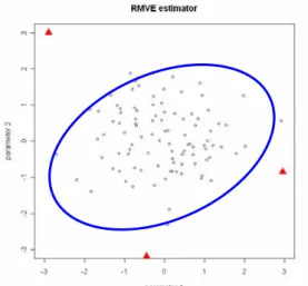
χ , the RMVE estimator robust to outliers. See Figure 2 for an illustration. We use the RMVE estimator in our monitoring statistic to detect out-of-control samples.
Figure 2: The triangle points are out of control, the solid ellipsoid is based on the RMVE estimator.
We use 2 RMVE
T , as our monitoring statistic and the control limit is obtained as follows: Step1: Without loss of generality, simulate m in-control profiles from multivariate normal
distribution with the mean vector μ 0 and covariance matrix = Σ = , where I is the I
identity matrix.
Step2: Compute estimator 2 RMVE
T in Equation (7).
Step3: Repeat step 1 and step 2 for N=100,000 times. Then the control limit is set as the empirical (1−α) ' quantify of the 100,000 values of 2
RMVE T , where 1 1 (1 )m I α = − −α , I
α is the percent false-alarm rate such that the overall false-alarm rate is approximately
3. A Study of the One-At-A-Time Scheme in Profile
Monitoring Scheme
3.1 Motivation
Williams, Birch, Woodall, and Ferry (2007) proposed a nonlinear profile monitoring method to monitor a set of Bioassay data. The bioassay data consists of forty-four weeks of in vivo bioassay results run alongside experimental compounds over a one-year time period. They removed 12 profiles. We wonder that some profiles of the removed profiles may be false alarms. Shiau and Sun (2006) proposed a one-at-a-time (OAAT) scheme for Phase I process monitoring that only discards the most extreme out-of-control sample at a time, using Shewhart X chart as an example, and demonstrate that the OAAT scheme reduces dramatically the occurrences of false alarms. So, we apply the OAAT scheme to nonlinear profile monitoring.
3.2 The OAAT Scheme
We describe the OAAT procedure (Shiau and Sun, 2006) below: Step 1. Construct the trial control limits with all of the collected data.
Step 2. If no out-of-control samples are identified, stop iterating and go to Step 4; otherwise, discard the most extreme sample.
Step 3. Construct the trial control limits with the remaining samples; go to Step 2.
Step 4. Collect all the samples discarded in the above iterations and inspect the process for assignable causes.
3.3 Simulation Studies
We use the parametric regression to model nonlinear profiles. Note that the 2 RMVE
T statistic in Equation (9) is invariant under the linear transformation. Thus, without loss of generality, we can simulate parameters from the multivariate normal distribution with mean vector μ 0 and = covariance matrix Σ = , where I is the identity matrix. Since over monitoring statistic I 2
RMVE
T is constructed based on the estimated parameter vectors of the profile, and the estimated parameter
are asymptotically nonlinear, and we simulate the parameter vectors direct from the multivariate normal distribution in comparing the OAAT and Delete-All schemes. In this way, we avoid interference of the estimation errors.
3.3.1 Simulation settings
For comparing the OAAT scheme and the Delete-All scheme. With the false-alarm rate and detecting power, we consider m=25(25)100, m1=3(3)12, p=2 and 4, and | δ |=1(1)20, where m is the number of profiles, m1 is the number of out-of-control profiles, p is the dimension, and | δ | is the length of δ (i.e., the mean of m1 profiles shifts from μ to μ δ ). For each combination, we + repeat 100,000 times and take averages of the 100,000 false-alarm rates and 100,000 detecting power respectively to estimate the actual values.
3.3.2 Results of Simulation Studies
The simulation result are summarized and displayed in Figures 2-11. We observe the followings from the simulation studies:
(1) From Figures 3 and 4, the false-alarm rate of the OAAT scheme is almost a constant and that of the Delete-All scheme is much higher, while the detecting power of both schemes are almost the same for p=2 and p=4.
(a) (b)
False-alarm rate ( m =25, m1 =3, and p =2)
0 0.005 0.01 0.015 0.02 1 3 5 7 9 11 13 15 17 19 Mean shift fal se-al ar m ra te Delete-All(p=2) OAAT(p=2) Power (m =25, m1 =3, and p =2) 0 0.2 0.4 0.6 0.8 1 1 3 5 7 9 11 13 15 17 19 Mean shift Po w er Delete-All(p=2) OAAT(p=2)
Figure 3: Comparisons of the OAAT scheme and Delete-All scheme for m1=3, m=25, and p=2 in terms of (a) the false-alarm rate, and (b) the detecting power.
(a) (b)
False-alarm rate ( m =25, m1 =3, and p =4)
0 0.002 0.004 0.006 0.008 0.01 0.012 0.014 0.016 0.018 1 3 5 7 9 11 13 15 17 19 Mean shift fal se-al arm rat e Delete-All(p=4) OAAT(p=4) Power (m =25, m1 =3, and p =4) 0 0.1 0.2 0.3 0.4 0.5 0.6 0.7 0.8 0.9 1 1 3 5 7 9 11 13 15 17 19 Mean shift Po wer Delete-All(p=4) OAAT(p=4)
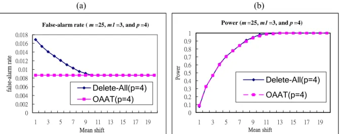
Figure 4: Comparisons of the OAAT scheme and Delete-All scheme for m1=3, m=25, and p=4 in terms of (a) the false-alarm rate, and (b) the detecting power.
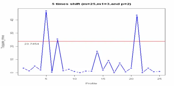
(2) The false-alarm rate of the Delete-All scheme decreases as |δ| increase. This is due to the fact that the RMVE estimator is more likely to be “contaminated” by out-of-control samples when the shift size is small. Then, the center of the ellipsoid is shifted, such that some in-control samples may be claimed as out of control. Figures 4 and 5 illustrate an example with |δ|=5 and 10, respectively. In this example, m=25, m1=3, p=2, |δ|=5, and the 5th, 14th, and 21st samples are the real out-of-control samples. Figure 5 shows that the 14th sample is not
detected and may have contaminated the RMVE estimator and causes the 7th sample to signal
a false alarm. But in Figure 6, with a larger shift size (|δ|=10), all these out-of-control samples are screened out by the RMVE estimator and then the 7th sample behaves normally.
Figure 5: An example with shift size |δ|=5.
Figure 6: An example with shift size |δ|=10.
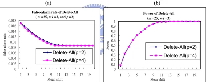
(3) Figures 7 and 8 compare the effect of p for the OAAT scheme and Delete-All scheme, respectively. For the OAAT scheme with p=2 or p=4, p shows almost no effects on both of the false-alarm rate and the detecting power. On the other hand, for the Delete-All scheme, Figure 8 presents a slight effect of p on the false-alarm rate, the smaller the dimension, the larger the false-alarm rate, but no effects on the detecting power.
(a) (b)
False-alarm rate of OAAT (m =25 and m 1=3) 0.00865 0.008651 0.008652 0.008653 0.008654 0.008655 0.008656 0.008657 0.008658 0.008659 0.00866 1 3 5 7 9 11 13 15 17 19 Mean shift false-ala rm ra te OAAT(p=2) OAAT(p=4) Power of OAAT (m =25 and m 1=3) 0 0.1 0.2 0.3 0.4 0.5 0.6 0.7 0.8 0.9 1 1 3 5 7 9 11 13 15 17 19 Mean shift Pow er OAAT(p=2) OAAT(p=4)
Figure 7: Effects of p on the OAAT scheme (a) The false-alarm rate, and (b) the detecting power for m1=3, m=25, and p=2, 4.
(a) (b)
False-alarm rate of Delete-All ( m =25, m1 =3, and p =2) 0 0.002 0.004 0.006 0.008 0.01 0.012 0.014 0.016 0.018 1 3 5 7 9 11 13 15 17 19 Mean shift fal se-al arm ra te Delete-All(p=2) Delete-All(p=4) Power of Delete-All (m =25, m1 =3) 0 0.1 0.2 0.3 0.4 0.5 0.6 0.7 0.8 0.9 1 1 3 5 7 9 11 13 15 17 19 Mean shift Power Delete-All(p=2) Delete-All(p=4)
Figure 8: Effects of p on the Delete-All scheme (a) The false-alarm rate, and (b) the detecting power for m1=3, m=25, and p=2, 4.
(4) From Figures 9 and 10 show that, when m increases, the false-alarm rate decreases and the detecting power increases for both of the OAAT scheme and the Delete-All scheme, which are expected.
(a) (b)
False-alarm rate of OAAT (p =2)
0 0.001 0.002 0.003 0.004 0.005 0.006 0.007 0.008 0.009 0.01 1 3 5 7 9 11 13 15 17 19 Mean shift fal se-a larm rat e m=25 (m1=3) m=50 (m1=6) m=75 (m1=9) m=100 (m1=12) Power of OAAT (p =2) 0 0.1 0.2 0.3 0.4 0.5 0.6 0.7 0.8 0.9 1 1 3 5 7 9 11 13 15 17 19 Mean shift Pow er m=25 (m1=3) m=50 (m1=6) m=75 (m1=9) m=100 (m1=12)
Figure 9: Effects of m on the OAAT scheme. (a) The false-alarm rate, and (b) the detecting power for m=25(25)100, m1=3(3)12, and p=2.
(a) (b)
False-alarm rate of Delete-All (p =2)
0 0.002 0.004 0.006 0.008 0.01 0.012 0.014 0.016 0.018 1 3 5 7 9 11 13 15 17 19 Mean shift fal se-al ar m ra te m=25 (m1=3) m=50 (m1=6) m=75 (m1=9) m=100 (m1=12) Power of Delete-All (p =2) 0 0.1 0.2 0.3 0.4 0.5 0.6 0.7 0.8 0.9 1 1 3 5 7 9 11 13 15 17 19 Mean shift Pow er m=25 (m1=3) m=50 (m1=6) m=75 (m1=9) m=100 (m1=12) Figure 10: Effects of m of the Delete-All scheme. (a) The false-alarm rate, and (b) the detecting
power for m=25(25)100, m1=3(3)12, and p=2.
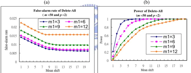
(5) From Figures 11 and 12, we observes that, when m1 increases, the false-alarm rate increases, the detecting power decreases for both of the OAAT scheme and Delete-All scheme, which is also expected.
(a) (b)
False-alarm rate of OAAT (p =2 and m =50)
0 0.002 0.004 0.006 0.008 0.01 0.012 0.014 0.016 0.018 1 3 5 7 9 11 13 15 17 19 Mean shift false-ala rm ra te m1=3 m1=6 m1=9 m1=12
Power of OAAT (p =2 and m =50)
0 0.2 0.4 0.6 0.8 1 1 3 5 7 9 11 13 15 17 19 Mean shift Po we r m1=3 m1=6 m1=9 m1=12
Figure 11: Effects of the proportion of out-of-control data on the OAAT scheme. (a) The false-alarm rate, and (b) the detecting power for m1=3(3)12, m=50, and p=2.
(a) (b)
False-alarm rate of Delete-All ( m =50 and p =2) 0 0.005 0.01 0.015 0.02 0.025 1 3 5 7 9 11 13 15 17 19 Mean shift fal se-al ar m ra te m1=3 m1=6 m1=9 m1=12 Power of Delete-All (m =50 and p =2) 0 0.2 0.4 0.6 0.8 1 1 3 5 7 9 11 13 15 17 19 Mean shift Po w er m1=3 m1=6 m1=9 m1=12
Figure 12: Effects of the proportion of out-of-control data on the Delete-All scheme. (a) The false-alarm rate, and (b) the detecting power for m1=3(3)12, m=50, and p=2.
To summary, it is found from the simulation studies, the OAAT scheme performs better than the Delete-All scheme because the OAAT scheme has a lower false-alarm rate and loses almost no detecting power. The only drawback of the OAAT scheme is that it is more complicated than the Delete-All scheme. In the next section, we provide a statistic to determine when to use the Delete-All scheme for real data, such that the process monitoring can be carried out more efficiently.
4. A Guideline for which Scheme to Use
By the simulation results presented in Section 3.3, we see that the OAAT scheme performs better than the Delete-All scheme in term of the false-alarm rate. But the OAAT scheme takes more time in computation than the Delete-All scheme. We also noted that the false-alarm rates for the two schemes are almost the same when the shift size is large. Therefore, if this situation happens, we may want to use the Delete-All scheme to save some time. Thus, one may like to have a guideline to decide which scheme to use. It is well known the median is robust to outliers while the mean is not. If the difference between the mean value and the median of data is large, it may imply that the shift is large and the out-of-control points are easy to detect. Then it might be safe to use the Delete-All scheme to save time. Otherwise, we will stick to the OAAT scheme.
4.1 Estimate the Real Variance from the Truncated Data
In Phase I analysis of the historical data set, it is wise to estimate the process parameters, say,
μ and σ2 with in-control data. Suppose we truncate off α(100)% of data, and use the
remaining data to estimate σ2, the estimator will be biased. We need a method to correct the bias.
If a normal distribution is truncated symmetrically about mean, then we have the relationship between the variances of the original distribution and the truncated distribution as
2 Var Y( )A
C
σ = (8)
where C= −1 2a aϕ( ) (2 ( ) 1),Φ a − Y is the truncated normal variate on A A= −[ a a, ],
1(1 2),
a= Φ− −α and ( )
A
Var Y is the variance of the truncated normal distribution with domain
.
A For the multivariate case, we also have C= −1 2a'ϕ( ) (2 ( ) 1)a Φ a' − with
' 1(( 1 1) / 2) a = Φ− p − +α , and A= Σ{ 1/ 2y*+μ | y*∈ −[ a a, ] }p with Y*∼N(0, ).I ( ) . Cov C Σ = YA (9)
The proofs are in the appendix. With equation (8) and (9), Tables 1-3 present respectively for 4 2, , 1 =
p , the values of the correction factor C for α =0.0027 ,0.05 ,0.1 ,0.5. For example, 2
,0.5
( A ) / 0.1426518
Var Y
σ = where Var(YA,α) is the variance of the truncated normal distribution with 50% truncation. And Σ =Cov(YA,0.5) / 0.3174066, where Cov(YA,0.5) is the covariance
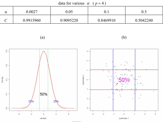
matrix of the truncated multivariate normal distribution with 50% truncation as shown in Figures 12 and 13. Thus, if we obtain an estimate of σ2from a set data with 50% trimming, than
we should divide it by C for bias correction. With equation (8) and (9), the variance or covariance can be estimated by the truncated normal distribution for (1−α)100% as described in Subsection 4.1 to avoid being affected by out-of-control data or outliers.
By Equation (8) and (9), Table 1-3 give, respectively for p=1, 2, and 4, the relationship between the variances of the normal distribution for various α . Thus an unbiased robust estimate of σ2 or Σ can be obtained through the in-control data from Phase I analysis.
Table 1: The value of C for bias correction of the variance estimated by the truncated normal data for various α (p=1)
α 0.0027 0.05 0.1 0.5
C 0.97333353 0.7588416 0.6230155 0.1426518
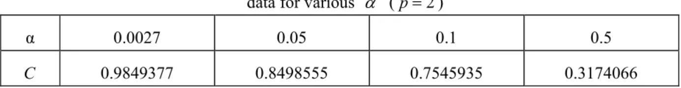
Table 2: The value of C for bias correction of the variance estimated by the truncated normal
data for various α (p=2)
α 0.0027 0.05 0.1 0.5
Table 3: The value of C for bias correction of the variance estimated by the truncated normal data for various α (p=4)
α 0.0027 0.05 0.1 0.5
C 0.9915960 0.9095220 0.8469910 0.5042240
(a) (b)
Figure 13: Truncated normal distribution with 50% truncated (α=0.5). (a) p=1, and (b) p=2.
4.2 The statistic for univariate data
We use the median of data (median(x)) to estimate μ, and use the σ2 for α =50% in Table 1 to estimate σ2.The statistic we propose here is
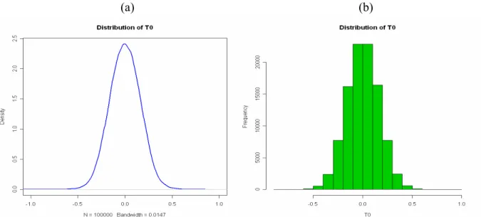
σˆ ) ( 0 x median x T = − , (10) where σˆ is the 50% “trimmed” estimate of σ as described in Subsection 4.1. Figures 14 and 15 display the kernel density estimate, a histogram, and the Q-Q plot of T0 obtained from 100,000 simulated samples of size m=100 from the standard normal distribution.
(a) (b)
Figure 14: The density plot of 100,000 simulated T0 values. (a) The density plot, and (b) the histogram plot.
Figure 15: The normal Q-Q plot for 100000 simulated statistic T0 .
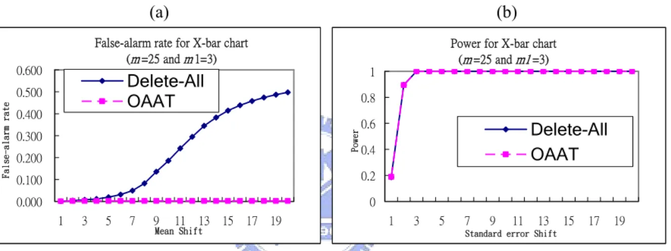
For the simulation studies, we observe one interesting thing. When the control chart under study has both upper and lower control limits, then the false-alarm rate of the Delete-All scheme will not come close to that of the OAAT scheme for larger shifts, which makes the OAAT scheme the only choice. See Figures 16-18 for examples of the two-tailed X , R, and S charts; and
Figures 19-20 for one-tailed R and S charts. The number of replications in the simulation is 100,000. Note that R (or S) chart is two-tailed when the subgroup is greater than 6. This can be explained by the following. Take the X chart as an example, when the shift size gets large, the center line gets higher, so does both of the control limits. But the width between two limits stays the same. Then many in-control points close to the LCL eventually will fall below the lower control limits. Figure 21 depicts this phenomenon. This situation will not happen for one-tailed control charts.
(a) (b)
False-alarm rate for X-bar chart (m =25 and m 1=3) 0.000 0.100 0.200 0.300 0.400 0.500 0.600 1 3 5 7 9 11 13 15 17 19 Mean Shift Fa ls e-al ar m ra te Delete-All OAAT
Power for X-bar chart (m =25 and m1 =3) 0 0.2 0.4 0.6 0.8 1 1 3 5 7 9 11 13 15 17 19
Standard error Shift
Po
we
r Delete-All
OAAT
Figure 16: Detect univariate data by X chart (two-tailed). (a) The false-alarm rate, and (b) the
detecting power.
(a) (b)
False-alarm rate for R chart (m =25 and m 1=3) 0.000 0.001 0.002 0.003 0.004 0.005 0.006 0.007 1 3 5 7 9 11 13 15 17 19
Standard error Shift
F als e-a lar m r ate Delete-All OAAT
Power for R chart (m =25 and m1 =3) 0 0.2 0.4 0.6 0.8 1 1 3 5 7 9 11 13 15 17 19
Standard error Shift
Pow
er Delete-All
OAAT
Figure 17: Detect univariate data by R chart and the subgroup is greater than 6 (two-tailed). (a) The false-alarm rate, and (b) the detecting power.
(a) (b)
False-alarm rate for S chart (m =25 and m 1=3) 0.000 0.001 0.002 0.003 0.004 0.005 0.006 0.007 1 3 5 7 9 11 13 15 17 19
Standard error Shift
Fa ls e-al arm r at e Delete-All OAAT
Power for S chart (m =25 m1 =3) 0 0.2 0.4 0.6 0.8 1 1 3 5 7 9 11 13 15 17 19
Standard error Shift
Po
we
r Delete-All
OAAT
Figure 18: Detect univariate data by S chart and the subgroup is greater than 6 (two-tailed). (a) The false-alarm rate, and (b) the detecting power.
(a) (b) F a l se -a l a rm ra te for R c ha rt (m =25 a nd m1 = 6) 0.0000 0.0005 0.0010 0.0015 0.0020 0.0025 0.0030 1 3 5 7 9 11 13 15 17 19 S t a n d a r d e r r o r S h i f t False-al
arm rate Delete-All
OAAT P owe r for R c ha rt (m =25 a nd m1 = 6) 0 0.2 0.4 0.6 0.8 1 1 3 5 7 9 11 13 15 17 19 S t a n d a r d e r r o r S h i f t Powe r Delete-All OAAT
Figure 19: R chart (one-tailed). (a) The false-alarm rate, and (b) the detecting power.
(a) (b)
False-alarm rate for S chart (m =25 and m1 =6) 0.0000 0.0005 0.0010 0.0015 0.0020 0.0025 0.0030 1 3 5 7 9 11 13 15 17 19
Standard error Shift
Fa lse -a lar m r at e Delete-All OAAT
Power for S chart (m =25 and m1 =6) 0 0.2 0.4 0.6 0.8 1 1 3 5 7 9 11 13 15 17 19
Standard error Shift
Po
we
r Delete-All
Figure 20: R chart (one-tailed). (a) The false-alarm rate, and (b) the detecting power.
(a) (b)
Figure 21: An example for X chart. (a) 10 times shift, and (b) no shift.
4.3. Simulation for univariate data
We need a cutoff point of T0 for decision making. Take R and S chart as examples. We simulate univariate data for different shifts δ=1(1)20, i.e., m1 profiles shift from σ to δσ . For each setting, we simulate m subgroups of size 5 to obtain m values of R and S. Then use Equation (12) to compute T0 for each of R and S. Repeat the above steps 100000 times to obtain 100,000 values of T0. Take the average of these T0’s. The combinations of (m, m1)=(25,3), (25,16), (100,12) are considered. Figure 22 shows the results. From Figure 22(a)(b), we observe that
(1) When m1 increases, T0 increases. (2) When m increases, T0 decreases. (3) When δ increases, T0increases.
(4) Compared with Figures 18 and 19 in which two false-alarm rate coincide around δ=14 for
R chart and δ=13 for S chart, we choose T0 =1 as the cutoff point. If T0 ≥ , then we use 1
(a) (b)
Figure 22: T0 for simulated univariate data. (a) R chart, and (b) S chart (one-tailed test).
4.4 The Statistic for Multivariate Data
For multivariate data, assume we have m profiles, each is represented by the estimated
parameter vector, with p by 1 parameter vectors, denoted by β , i=1,2,…,m. Without loss of i
generality, we simulate parameters β from the multivariate normal distribution with the mean i
vector μ=0and covariance matrix Σ = , where I is the identity matrix. Denote β the mean I
of β ’s, and i median β the componentwise median of ( )i β ’s. Let S be the “trimmed” i
covariance matrix estimate described in Subsection 4.1. We use the following statistic
0
2 ( ( )) ' 1( ( )),
i i
T = β−median β S− β−median β (11)
to determine which scheme to use.
We simulate multivariate data with mean vector μ=0 and covariance matrix Σ = (p=2 I
and m=100), and repeat 100,000 times. We plot the density, histogram and chi-square Q-Q plot of
these 100,000 values of 2 0
T in Figures 23 and 24. It might be reasonable to assume that the 2 0
statistic has a approximate scaled chi-square distribution with p degrees of freedom.
(a) (b)
Figure 23: The plot of the statistic 2 0
T from simulated multivariate data. (a) The density plot, and (b) the histogram plot.
Figure 24: The chi-square Q-Q plot for the statistic 2 0
4.5 Simulation for multivariate data
We simulate multivariate data with different shifts (|δ|=1(1)20). Similar to the unvariate case,
we use Equation (11) to compute 2 0
T . According to Figure 25 and 26, we observe that
(1) When p increases, 2 0
T increases. (2) When m1 increases, T02 increases. (3) When m increases, 2 0 T decreases. (4) When δ increases, 2 0 T increases.
(5) By the same argument as before, we choose to use the Delete-All scheme when 2 0 1
T ≥ and the OAAT scheme, when 2 1
0 <
T ..
Figure 25: 2 0
(a) (b)
Figure 26: 2 0
T for simulated multivariate data. (a) p=2, and (b) p=4.
To summary, we recommend always use the OAAT scheme when the control chart has both upper and lower control limits. For one limit control chart, when the 2
0 (or ) 10
T T ≥ , then use the Delete-All scheme to save time.
5. Examples
5.1 Bioassay Data
5.1.1 Data Description
To compare the profile monitoring schemes between the OAAT and the Delete-All schemes, we analyze the data from DuPont Crop Protection (Woodall, Williams, Birch, and Ferry, 2007). The data set consists of forty-four weeks (m =44) of in vivo bioassay results run alongside
experimental compounds over a one-year time period.
The commercial compound was diluted to eight doses (0.003, 0.009, 0.028, 0.084, 0.25, 0.76, 2.27, and 6.8 (d=8)) and replicated four times at each dose (r = 4) in 96-well microtiter plates for
each sampling period i. A spectrophotometer measured the optical density (OD) of the plant
organism after the inoculation period.
Let yijk represents the kth response to the jth dose at sampling period i, where i = 1,2, …,m , j =
1,2,…,d, and k = 1,2,…, r. For this data set, we have m = 44, d = 8, and r = 4. Both treated and
untreated wells were measured for growth inhibition. The percent control (PC) values were
calculated using the median OD (Mi) from 96 replications of untreated wells. Williams, Woodall, Ferry, and Birch (2007) let Mi represent the median response of the untreated specimen at sampling period i. Then, the percent control of the chemical for the kth replication of the jth dose in sampling period i is calculated as
, 1,..., , 1,..., , 1,.., . i ijk ijk i M y PC i m j d k r M − = = = = (12)
A plot of PCijk values for all m = 44 weeks for one of the standards from the DuPont is given in Figure 27. Because the bioassay data have replications (r = 4), we need to first monitor the variance within profiles. Williams, Woodall, Ferry, and Birch (2007) referred to it as the variance profile monitoring.
5.1.2 Monitoring for Bioassay Data
We analyze the profiles in the bioassay data in Figure 27 and consider the following 4-parameter logistic model which has been used frequently for dose-response studies (Williams, et al. (2007)): , 1,..., , 1,.., , 1 ( ) i i i ij i ij ij B i D A y A i m j n x C ε − = + + = = + (13)
where A is the upper asymptote, i D is the lower asymptote, i C is the point where the curve i
reaches halfway between A and i D , and i B is a parameter representing the rate of increase or i
decrease from D to i A in Figure 28. Since the estimators of i A , i B , i C , and i D are i
correlated, it is more appropriate to account for the correlation among them when testing for unusual values of ˆA , ˆi B , ˆi C and ˆi D . We illustrate the estimated mean profiles for all i
forty-four weeks in Figure 29.
We use the RMVE in Equation (7) to monitor dose-response profiles. As a result, both the OAAT and Delete-All schemes remove the same 13th, 20th, 21st, 22nd, 24th, 26th, 32nd, 34th, 45th,
46th, and 48th profiles in the end. See Figure 30 (a) gives the control chart of the first iteration and
30(b) shows the result of the last iteration in which the remaining 33 profiles are in control.
(a) (b)
Figure 30: The RMVE chart when monitoring unusual profiles. (a) The 44 dose-response profiles at the first iteration, and (b) the 33 dose-response profiles at the last iteration.
We compute the 2 0
T statistic according to Equation (11) for the original 44 profiles and find that 2
0
T =0.992673, very close to the suggested cutoff value 1. The result that both schemes
removed the same set of the profiles is in accordance with the result that 2 0
T is close 1.
For demonstrating that the OAAT scheme performs better than the Delete-All scheme, we use the variance profile monitoring of Williams, et al. (2007). Since there are 4 replications at every dose j, estimate 2
ij
2 2 1 ( ) ˆ . 1 ij ijk k ij ij PC PC S r σ = − = = −
∑
(14)Following Williams, et al. (2007), we model ˆ2 ij σ by the model 2 2 0, 1, ˆ ( ij) ( )ij i i ( ).ij
log σ =log S =θ +θ log x (15)
Figure 31 displays the fitted results of the 44 variance profiles.
We use the RMVE statistic in Equation (7) to monitor the variance profiles. The OAAT scheme removes only the 20th and 45th weeks in Figure 32(a)(b), and the Delete-All scheme first
removes 6th, 20th, 22nd, 24th, 26th, and 45th weeks and then removes 16th, 19th, 34th and 44th again.
See Figure 33(a)(b)(c), respectively. The OAAT scheme has 42 profiles remaining, and the Delete-All scheme has only 34 profiles left. It is apparent that the Delete-All scheme removes a lot more than the OAAT scheme. It could be a reasonable doubt that the Delete-All scheme picks come false-alarms.
(a) (b)
Figure 32: The RMVE chart when monitoring the remaining variance profiles by the OAAT scheme. (a) The 44 variance profiles, and (b) the 42 variance profiles.
(a) (b)
(c)
Figure 33: The RMVE chart when monitoring the remaining variance profiles by the Delete-All scheme. (a) The 44 initial variance profiles, (b) the 38 variance profiles, after the 1st iteration, and (c) the remaining 34 variance profiles.
Note that the 2 0
T value for the variance profiles is 0.2747621, indicating it is likely that some false-alarms are signaled by the Delete-All scheme.
After removing the profiles that signal out of control in the variance profiles monitoring, we monitor the remaining dose-response profiles. For the 42 remaining profiles, the OAAT scheme removes 13th, 21st, 22nd, 24th, 26th, 32nd, 34th, 46th, and 48th weeks, and see Figure 34(a)(b). For the remaining 34 profiles, Delete-All scheme first removes 13th, 32nd, and 48th weeks, then removes 21st, and 46th weeks, see Figure 35(a),(b), and (c), respectively. At the end, the remaining
33 profiles by the OAAT scheme, and the remaining 29 profiles by the Delete-All scheme, are in control now.
(a) (b)
Figure 34: The RMVE chart when monitoring the remaining mean profiles by the OAAT scheme. (a) The 42 mean profiles, (b) the 33 mean profiles.
(c)
Figure 35: The RMVE chart when monitoring the remaining mean profiles by the Delete-All scheme. (a) The 34 mean profiles, (b) the 31 mean profiles, and (c) the 29 mean profiles.
Are the additional 6th, 16th, 19th, and 44th profiles signaled by the Delete-All false-alarm rate?
To see this, we plot 44 profiles in Figure 36 with these four profiles highlighted. The 6th, 16th, and 19th profiles seem fairly normal. But the 44th profile seems somewhat unusual, and the OAAT scheme does not remove it. The reason might be that 4 parameters A, B, C, and D of this profile are monitored equally weighted by RMVE. Although the parameter B of the 44th profile is smaller than the other profiles, the parameters A, C, and D are fairly similar to that of other in-control profiles. Thus the difference in B becomes insignificant in the overall measure 2
RMVE
T . If we want to emphasize a particular feature like the increasing rate represented by B, we may consider put more weights on that component.
Figure 36: The thick lines are the 6th, 16th, 19th, and 44th profiles.
5.2 Vertical Board Density Data (VDP)
5.2.1 Data Description
Manufacturers of engineered wood boards, which include particleboard and medium density fiberboard, are very concerned about the density properties of the board produced. The density is measured using a profilometer which uses a laser device to take a series of measurements across the thickness of the board. A profilometer takes multiple measurements on a sample (usually a
2x2 inch piece) to form the vertical density profile (VDP) of the board.
Vertical Board Density Profile Data from Walker and Wright (2002) contains 24 profiles of vertical density, each profile consists of 314 measurements, see Figure 37.
We model the VDP profiles, different form that William, et al. (2003), as follows: c d x a f(xi,β)= ij− b + (16)
where i=1,..,24 and j=1,…314. Let β=( , , , )'a b c d , where a represents the height of the “bathtub”,
b controls the “flatness” of the “bathtub”, c is the bottom of the “bathtub”; and d is the center of
them in Figure 38.
5.2.2 Monitoring the VDP Data
We use the RMVE chart in Equation (9) to monitor the VDP profiles. The results are as follows. Both the OAAT and the Delete-All schemes remove the 4th, 9th, 17th, 20th, and 24th
profiles, see Figure 39(a)(b). Figure 39(c) shows that the remaining 18 profiles are now in control. For saving computing time, we suggest using the Delete-All scheme to the VDP data.
(a) (b)
(c)
Figure 39: The RMVE chart when monitor VDP profile. (a) The 24 boards at the first iteration, (b) the 22 boards at the 2nd iteration, and (c) the 18 boards at the final iteration.
We compute the 2 0
T statistic for the VDP data, and find that 2 0
T = 4.622674. With 2 0
large, we could just use the Delete-All scheme to monitor profiles. Figure 40 shows all 24 filled profiles by the model (16). We notice that the highest board (the 3rd board) and the lowest board
(the 6th board) are not removed by both schemes. The same argument about the 44th profile of the
response-dose data may be applied here.
Figure 40: The 3rd and 6th profiles are not removed.
5.3 The
T Statistic for Examples
02We compute the 2 0
T statistic for the bioassay data by Equation (9). The 2 0
T statistic is 0.992673 for does-response profile monitoring. Although 0.992673 is almost equal to the cutoff point 1.0, for being conservative, we suggest using the OAAT scheme. The 2
0
T statistic is 0.2747621 for the variance of profiles monitoring, so we should use the OAAT scheme.
For the VDP data, the 2 0
T statistic is 4.622674, which is so large that we could just use the Delete-All scheme. Hence, before monitoring real data we may use the statistic in Equation (8) and (9) to decide which scheme to use.
In summary, the results of these two examples agree with the decision criterion 2 0
T . The
Bioassay data in Subsection 5.1 demonstrate a case that the OAAT scheme performs better than the Delete-All scheme while the VDP example in Subsection 5.2 demonstrates a case that we could use the Delete-All scheme to save some computing.