國立交通大學
應用數學系數學建模與科學計算碩士班
碩 士 論 文
利用混沌序列模擬樹的樣態
Tree Patterns Simulated by Chaotic Sequences
研 究 生:林育賢
指導教授:張書銘 博士
利用混沌序列模擬樹的樣態
Tree Patterns Simulated by Chaotic Sequences
研 究 生:林育賢
指導教授:張書銘 博士
Student: Yu-Hsien Lin
Advisor: Dr. Shu-Ming Chang
國 立 交 通 大 學
應 用 數 學 系
數 學 建 模 與 科 學 計 算 碩 士 班
碩 士 論 文
A Thesis
Submitted to Department of Applied Mathematics College of Science,
Institute of Mathematical Modeling and Scientific Computing
National Chiao Tung University
in Partial Fulfillment of the Requirements
for the Degree of
Master
in
Applied Mathematices
June 2010
Hsinchu, Taiwan, Republic of China
利用混沌序列模擬樹的樣態
學生:林育賢
指導教授:張書銘
博士
國立交通大學應用數學系
數學建模與科學計算所碩士班
摘
要
本論文簡短地說明碎形 (fractal) 與混沌 (chaos) 在模擬自然界現象上的使用。憑藉著自我 相似性,碎形被廣泛的使用在模擬樹與花草等自然界物質。在碎形樹的模擬中,遞迴函數 系統 (iterated function system) 最為普遍。此外,交大通識中心陳明璋教授並根據遞迴函 數系統發展出結構複製法 (structural cloning method) 進而開創視覺碎形的新領域。本研究 著重於三個均勻分布生長機制:邏輯斯諦映射 (logistic map)、修正邏輯斯諦映射 (modified logistic map) 與偽隨機數生長器 (pseudorandom number generator) 對於樹樣態模擬中生長 變數的調控,並且發展兩種不同的模擬機制:樹生成模擬 (Grown Tree Simulation) 與樹生 長模擬 (Growing Tree Simulation),完全破壞碎形樹的自我相似性,呈現多樣化的面貌。 此外,本論文最後利用統計檢定的方式,對於各種不同模擬或生長機制下的樹進行比較與 結果分析,在不同的結果之間提供更客觀的詮釋。Tree Patterns Simulated by Chaotic Sequences
Student: Yu-Hsien Lin
Advisors: Dr. Shu-Ming Chang
Institute of Mathematical Modeling and Scientific Computing National Chiao Tung University
1001, Ta Hsueh Road, HsinChu 300 Taiwan
June, 2010
Abstract
This study gives a brief description of fractals and chaos used in the real world, es-pecially in the nature world. Fractals, by its self-similarity, has widely used to simulate things such as trees and cloudes. Besides, one of the most common ways to generate fractals is iterated function system (IFS). On the basis of IFS, Dr. Ming-Jang Chen developed Structural Cloning Method (SCM) which is regarded as an original frontier of visual fractals to simulate trees, mountains and so on. In this thesis, unlike IFS and SCM, we focus on the tree pattern simulations by three uniformly distributed generators, pseudorandom number generator, logistic map generator and modified logistic map gen-erator in order to break the self-similarity of fractal trees and whether there are stronger links between chaotic sequences and the trees in the real world. Moreover, there are two simulations proposed here: Grown Tree Simulation and Growing Tree Simulation. They take diverse views on simulating the tree patterns. In this way, there are at least six different kinds of models. At this background, these models should be compared by a more persuasive way than just by sights and preference. Thus, hypothesis tests offer an alternative interpretation in the end.
Keywords: logistic map, modified logistic map, iterated function systems, structural cloning
誌
謝
本篇論文的完成,最感謝我的指導老師張書銘 教授,不論學術上的指導與人生
道理的教誨,我堅信所受得的這些將會是我未來人生裡受用無窮的資源。並且同時
感謝我的口試委員莊重 教授和陳明璋 教授,於口試時給予當頭棒喝的提醒。
這 篇 論 文 的 誕 生,特 別 感 謝 一 路 上 不 吝 給 我 指 導 還 有 提 供 協 助 的 人,
扣斯、鄭仲元、便便、茵妮、賴淑俐、雅雯、15B、柏新、庫比、潘帥、BBN、暉哥、
段俊旭、吳啟豪,無法獨立完成的部分,都是因為你們的協助才得以完成。
兩年來的日子裡,謝謝建模所與數學系的同學相伴與指點,緣分雖然不長,卻也
開啟了我另一頁的生活篇章。研究生涯苦悶,很開心依然可以認識到新的人,給予
生活另一種視野,也很開心我的老朋友們仍在我的身邊,多難熬的時候,總是給我
溫暖的陪伴。
謝謝我的家人,這些年來我學會獨立自主,學會了堅強承擔,都必須感謝你們的
愛與包容。今日所有的成長,與你們一起分享。
林育賢 謹誌于交通大學 2010 年 6 月Contents
1 Introduction 1
2 Preliminaries 3
2.1 Pseudorandom Number Generator . . . 3
2.2 Logistic Map . . . 4
2.3 Modified Logistic Map . . . 5
3 General Ideas of Modeling Natural Trees 5 3.1 Coordinates of Each Node . . . 5
3.2 The Role of the Generators in the Models . . . 7
4 Scheme for Principle Processes 7 4.1 Algorithms of Trees Modeling . . . 9
4.2 Design for Statistical Analysis . . . 11
5 Simulation Results 13 5.1 Results of the Proposed Tree Models . . . 13
5.2 Statistical Analysis . . . 36
5.2.1 Two-Sample Hypothesis Tests . . . 36
5.2.2 Results of Statistical Analysis . . . 37
5.3 Summary . . . 52
6 Conclusions and Future Works 53
List of Figures
1.1 A simple tree produced by IFS. . . 2
2.1 Varied behavior for logistic map . . . 4
5.1 Some trees made by IFS . . . 15
5.2 Some trees made by Grown Tree Simulation with PRNG . . . 16
5.3 Some trees made by Grown Tree Simulation with LMG; γ = 4 . . . 17
5.4 Some trees made by Grown Tree Simulation with LMG; γ = 3.98 . . . 18
5.5 Some trees made by Grown Tree Simulation with LMG; γ = 3.8 . . . 19
5.6 Some trees made by Grown Tree Simulation with MLMG; γ = 4.1 . . . 20
5.7 Some trees made by Grown Tree Simulation with MLMG; γ = 36.9 . . . 21
5.8 Some trees made by Grown Tree Simulation with MLMG; γ = 53 . . . 22
5.9 Some trees made by Growing Tree Simulation with PRNG . . . 23
5.10 Some trees made by Growing Tree Simulation with LMG; γ = 4 . . . 24
5.11 Some trees made by Growing Tree Simulation with LMG; γ = 3.98 . . . 25
5.12 Some trees made by Growing Tree Simulation with LMG; γ = 3.8 . . . 26
5.13 Some trees made by Growing Tree Simulation with MLMG; γ = 5 . . . 27
5.14 Some trees made by Growing Tree Simulation with MLMG; γ = 23 . . . 28
5.15 Some trees made by Growing Tree Simulation with MLMG; γ = 53.3 . . . 29
5.16 A growing tree made by Growing Tree Simulation with PRNG . . . 30
5.17 A growing tree made by Growing Tree Simulation with LMG . . . 31
5.18 A growing tree made by Growing Tree Simulation with MLMG. . . 32
5.19 A growing tree made by Growing Tree Simulation with PRNG . . . 33
5.20 A growing tree made by Growing Tree Simulation with LMG . . . 34
5.21 A growing tree made by Growing Tree Simulation with MLMG. . . 35
5.22 Brief procedure of the boundary decided one of the samples . . . 47
5.23 Some photos took in the real world to be the sample data . . . 48
5.24 Brief procedure of the boundary of a tree photo sample decided . . . 49
5.25 Brief procedure of the boundary of a sample made by IFS decided . . . 50
List of Tables
3.1 The coordinate of the trunk; c0 = l . . . 8
3.2 The coordinate of the 1st and 2nd layer of the branches, where 1 ≤ i
1, i2 ≤ β . 8
3.3 The coordinate of the nth layer of the branches, where 1 ≤ i
1
Introduction
The concepts of chaos and fractals have received widespread attention in recent years among mathematicians, scientists, graphic designers and so on. Also, they are quite developing in the wide range of areas. For instance, chaos and fractals are used in forecasting movements in foreign exchange and stock markets to understand international business cycles [11]. Even a marriage relationship can be connected with the theory of chaos and fractals as well [9].
Mathematically, chaos is defined as “randomness” generated by simple deterministic sys-tems. This randomness is a result of the sensitivity of chaotic systems to the initial system. That is to say, infinitesimal variations in initial conditions for a chaotic dynamic system lead to large variations in behavior. However, because the systems are deterministic, chaos implies some order. They are actually deterministic systems governed by physical or mathemati-cal laws, and so are completely predictable given perfect knowledge of the initial conditions. Furthermore, chaotic behavior can be observed in many natural systems, such as Lorenz’s equation, which provides scientists a significant way of looking at the complexity in climate change [3,21, 22].
Moreover, a fractal is an indivisible part of the theory of dynamical systems and chaos. It is a geometrical figure in which an identical motif repeats itself on an ever diminishing scale [10]. Its godfather is the Franco-American mathematician Benoit B. Mandelbrot. In the 1960s and 1970s, as an IBM researcher, Benoit B. Mandelbrot invented a new geometry, which he called “fractal” geometry [13,14]. It pushed deeply into this frontier. He coined the term “fractal” to suggest “fractured” and “fractional” –a geometry that focuses on broken, wrinkled, and uneven shapes. In truth, we see fractals every day, such as trees, mountains, and the scattering of autumn leaves. All these are fractal patterns, signs of dynamical activity at work. Chaos theory tells the story of the wild things that happen to dynamical systems as they evolve over time; fractal geometry records the images of their movement in space. In brief, fractal geometry is the pattern of the behavior of chaos [3, 12].
Fractals have one notable quality that they are self-similar on multiple scales, in that a small portion of a fractal will often look similar to the whole object, much as a fern leaf looks very much like a fern tree. Also, scale invariance is an exact form of self-similarity where at any magnification there is a smaller piece of the object that is similar to the whole. Because of self-similar, all fractals have a built-in form of recursion. Sometimes the recursion is explicit visible in how the fractal is constructed. Other times the recursion is a little more subtle and may be an artifact of an underlying fractal-building process that occurs on multiple spatial
scales. The first type of fractal can typically be defined by a program-like specification such as the Cantor set, while the other is usually related to a random or stochastic process such as Brownian motion and some nature phenomena [2, 8].
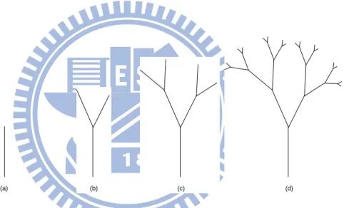
It is obvious to see that not all of nature phenomena such as trees, coastlines, snow flakes, and clouds, are adequately described by straight lines, curves, or even pure fractals. Nevertheless, they can be modeled on a computer by using recursive algorithms. Iterated function system (IFS) [1, 17] is one of the most common ways of generating fractals. Take a tree for example, IFS is shown in Figure 1.1. We start with a simple branching rule, growing two branches from a trunk. The lengths of the branches are to be less than the length of the trunk, and the angles between the lines of the trunk and the branches are given. Then treat the branches as trunks and do the same branching again at their ends. After some times of iterations, it displays a treelike graph.
(a) (b) (c) (d)
Figure 1.1: A simple tree produced by IFS
In 2004, Ming-Jang Chen [5], vice-professor of Center for General Education in National Chiao Tung University, developed Structural Cloning Method (SCM) to simulate trees, clouds, flowers, mountains, stones in the nature world. SCM, regarding IFS as its foundation, keeps the self-similarity and the repetition of fractals as well. SCM also claims that it developed an original frontier of visual fractals, which is distinct from views of mathematical fractals and natural fractals. Thus, SCM makes a milestone of the field of Computer drafting.
In this thesis, we proposed new methods to simulate trees in the real world. Instead of SCM, we try to break the self-similarity of the IFS which is composed with itself, starting from some initial value and repeat it over and over again. This thesis takes the assumption that the nature phenomena exactly conform to fractals as idealized abstraction. However, it does not mean fractals would be put aside in the thesis. Instead, on the basis of fractal trees,
we reconstruct them with three generators which take on uniform distribution expecting to meet the complexity in the real world even more closely than previous work.
The rest of the thesis is organized as follows. The background of this work is briefed in section 2. General ideas about modeling trees in the nature world are presented in section 3. The scheme of this research is introduced in section 4. Simulation results are summarized and remarked in section 5. Section 6 concludes the paper and addresses some future work.
2
Preliminaries
In this section, three uniformly distributed generators, pseudorandom number generator, logistic map, as well as modified logistic map, are introduced.
2.1
Pseudorandom Number Generator
A pseudorandom number generator (PRNG) is an algorithm for generating a sequence of numbers that approximates the properties of random numbers. Randomness is often used in statistics to signify well-defined statistical properties, such as a lack of bias or correlation. Namely, random implies a lack of predictability. However, the sequence made by PRNG is not truly random in that it is completely determined by a relatively small set of initial values, called the PRNG’s state. Although sequences that are closer to truly random can be generated using hardware random number generators which is an apparatus that generates random numbers from a physical process, pseudorandom numbers are important in practice for simulations and are central in the practice of cryptography and procedural generation [19]. In this research, this generator is produced by the MATLAB pseudorandom number generator. In Numerical Computing with MATLAB [18], it gives a clear description of what the algorithms for PRNGs in MATLAB is doing. In brief, MATLAB introduces a random number generator whose algorithm is based on the work of George Marsaglia [15], a professor at Florida State University and author of the classic analysis of random number generators, “Random numbers fall mainly in the planes”. The random number generators would be almost completely satisfactory, because Marsaglia has shown that it has a huge period – almost 21430 value would be generated before it repeated itself. Besides, MATLAB modifies
the generator a little bit and the period of which becomes something like 21492. In any case,
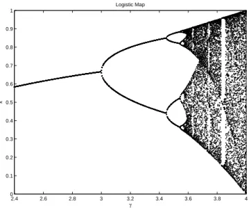
2.4 2.6 2.8 3 3.2 3.4 3.6 3.8 4 0 0.1 0.2 0.3 0.4 0.5 0.6 0.7 0.8 0.9 1 γ x Logistic Map
Figure 2.1: Varied behavior for logistic map
2.2
Logistic Map
A logistic map (also known as the “quadratic map” or the “Feigenbaum map”) [7,8,16,17,20] which is a model for the growth of an idealized population consisting of only one species is defined by the iterated equation
xn+1= γxn(1 − xn), (2.1)
where:
• xn is a number between 0 and 1, and represents the population at year n, and hence x0
represents the initial population (at year 0).
• γ is a positive number, and represents a combined rate for reproduction and starvation.
Using this formula, the population is in the succeeding generation can be deduced from a knowledge of only the population in the preceding generation and the constant γ. By varying the parameter γ, it reveals variety of results of the system and tends to measure the population of the species at the end of each generation. However, this system is unpredictable by nature, because any small change produces a vastly different eventually values for xn (Figure2.1). In
fact, it has shown that equation (2.1) has chaotic behavior for 3.57 < γ ≤ 4. In the interval, the generated sequence of the logistic map is non-periodic.
Thus, the selection of γ as the generator is limited. The set of visualized chaos is small and sparse for γ ∈ (3.57, 4). However, for γ ∈ (3.57, 4), the chaotic attractor — an object toward
which all nearby solutions tend even if slightly disturbed as time moves on— is not distributed within the range of 0 and 1. The best case of equation (2.1) as logistic map generator (LMG) may be when γ = 4 not only because it has chaotic behavior, but also because its chaotic attractor is uniformly distributed in the range of 0 to 1.
2.3
Modified Logistic Map
In 2009, Chang and so on proposed a modified logistic map (MLM) which is developed from a classical logistic map [4, 6]. MLM is defined as follows:
L(γ, x) = γx(1 − x)(mod 1), x ∈ Iext, γx(1 − x)(mod 1) γ 4(mod 1) , x ∈ Iint, (2.2)
where Iext ∈ (0, 1)\Iint, Iint = [η1, η2], η1 = 12 −
q 1 4 − [γ4] γ and η2 = 1 2 + q 1 4 − [γ4] γ in which [z]
is the greatest integer less than or equal to z. MLM is then defined by x(i+1) = L(γ, xi).
For γ ≤ 4 , the behavior of MLM is equivalent to the classical logistic map, equation (2.1) at γ = 4 which is chaotic in the case. Hence, the sequence generated by the MLM never settles down to a fix point or a periodic orbit. Namely, it reveals the aperiodic long-time behavior. Also, it has been shown that when γ ≥ 4 , L(γ, x) has chaotic behavior which is topologically equivalent to that of γ = 4, and is uniformly distributed in the range of 0 to 1. Therefore, any value not smaller than 4 for γ can be selected in MLM to be our modified logistic map generator (MLMG).
3
General Ideas of Modeling Natural Trees
In order to construct our model of trees, we assume that a tree is composed of trunk and branches which are all straight lines. In the first place, we use coordinates to establish position of each node which stands for the startpoint and endpoint of each branch. Then, the angle and length of a branch is set by generators introduced previously. In this section, it will give more specific description of the general ideas of constructing our models.
3.1
Coordinates of Each Node
For the sake of setting the coordinates of each startpoint and endpoint, we define that: A tree is composed of a trunk and branches with n-layers and they are all supposed to be
straight lines. where:
• l: the length of the trunk.
β: the maximum number of branches at one layer. A0: the x-coordinates of the startpoints of the trunk.
B0: the y-coordinates of the startpoints of the trunk.
C0: the x-coordinates of the endpoints of the trunk.
D0: the y-coordinates of the endpoints of the trunk.
• Ai1,i2,...,in: a value stand for the x-coordinates of the startpoints of a specified branch at
the nth layer.
Bi1,i2,...,in: a value stand for the y-coordinates of the startpoints of a specified branch at
the nth layer.
Ci1,i2,...,in: a value stand for the x-coordinates of the endpoints of a specified branch at
the nth layer.
Di1,i2,...,in: a value stand for the y-coordinates of the endpoints of a specified branch at
the nth layer.
• ai1,i2,...,in: a value stand for the lengths of a specified branch at the n
th layer.
ci1,i2,...,in: a value stand for the lengths from root to bifurcation node of a specified
branch at the (n − 1)th layer .
θi1,i2,...,in: a value stand for the angles with respect to the horizontal line of a specified
branch at the nth layer.
• Some restrictions: 0 < ai1,i2,...,in < l.
0 < ci1,i2,...,in < l.
0 < θi1,i2,...,in < π.
0 < i1, i2, ...in≤ β , and i1, i2, ...in ∈ Z.
In addition, the value of index i1, i2, ..., in represents the sequence of bifurcating. Take a3,4,1
for example, it represents that the length of the branch, which is the number three bifurcation at first layer, the number four bifurcation at second layer and then the number one bifurcation at the third layer.
The general forms of coordinates of the startpoints and endpoints in the models are shown in Table 3.1, 3.2 and 3.3.
3.2
The Role of the Generators in the Models
In IFS, once the trunk and each branch at layer 1 are given, they will be duplicated to form a tree. Just because of the characteristic of self-similarity, the three variables, ai1,i2,...,in, ci1,i2,...,in
and θi1,i2,...,in, follow their own recurrence relations. They are listed as below.
The recurrence relations:
ai1,i2,...,in = ai1,i2,...,in−1 × ain l , (3.1) ci1,i2,...,in = ci1,i2,...,in−1× cin l , (3.2) θi1,i2,...,in = θi1,i2,...,in−1 + θin− π 2. (3.3)
The general forms:
ai1,i2,...,in = ai1 × ai2 × ai3 × ... × ain ln−1 , ci1,i2,...,in = ci1 × ci2 × ci3 × ... × cin ln−1 , θi1,i2,...,in = θi1 + θi2 + ... + θin − (n − 1) × π 2.
In equation (3.1), the ratio of ain to l plays an important part in the recurrence relations.
Same as that in equation (3.2), the value of ci1,i2,...,in is also decided by the ratio of cin to
l. However, in order to prevent self-similarity in our trees, these rules do not apply here. Namely, even the trunk and branches at layer 1 are given, it could display variety of results in our model as well. Take ai1,i2,...,in for instance, generators function here to make its value.
After generators affect it, the only restriction becomes ai1,i2,...,in ≤ ai1,i2,...,in−1. That is to say,
there is no fixed ratio between the length of one branch at layer n and which at its previous layer. Also, generators work in ci1,i2,...,in and θi1,i2,...,in. It breaks some close connection with
these variables. Apparently this difference from IFS makes this model take on an infinite variety of form. To be more specific, the detailed method will be introduced in next section.
4
Scheme for Principle Processes
This section will introduce the complete process design for the models constructing and results analysis. First, the proposed algorithms are designed to simulate trees in the real world more
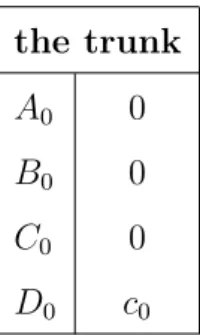
the trunk A0 0
B0 0
C0 0
D0 c0
Table 3.1: The coordinate of the trunk; c0 = l
1st layer 2nd layer Ai1 0 Ai1,i2 ci1,i2cos θi1
Bi1 ci1 Bi1,i2 ci1 + ci1,i2sin θi1
Ci1 ai1cos θi1 Ci1,i2 ci1,i2cos θi1 + ai1,i2cos θi1,i2
Di1 ci1 + ai1sin θi1 Di1,i2 ci1 + ci1,i2sin θi1+ ai1,i2sin θi1,i2
Table 3.2: The coordinate of the 1st and 2nd layer of the branches, where 1 ≤ i1, i2 ≤ β
nth layer (n≥ 3)
Ai1,i2,...,in k=n
P
k=3
ci1,i2,...,ikcos θi1,i2,...,ik−1
Bi1,i2,...,in ci1 + ci1,i2sin θi1 + k=n
P
k=3
ci1,i2,...,iksin θi1,i2,...,ik−1
Ci1,i2,...,in k=n
P
k=3
ci1,i2,...,ikcos θi1,i2,...,ik−1 + ai1,i2,...,incos θi1,i2,...,in
Di1,i2,...,in ci1 + ci1,i2sin θi1 + k=n
P
k=3
ci1,i2,...,iksin θi1,i2,...,ik−1+ ai1,i2,...,insin θi1,i2,...,in
Table 3.3: The coordinate of the nth layer of the branches, where 1 ≤ i
diverse than IFS. There are two methods of constructing the models in two dissimilar aspects. With three generators operating in each model, at least six kinds of algorithms are proposed here. Next, comparing all these results with one another,which made by IFS and trees in the real world is also a topic. Statistical hypothesis testing backs these up.
4.1
Algorithms of Trees Modeling
We develope two methods to model the trees in this thesis. The first one directly simulates the appearances of grown trees, while the other tends to show trees under growing with dynamic behavior. However, without the former, the later could not be finished. It can be said that the latter is succeeded by the former. Also, we refer the first method as Grown Tree Simulation, and the second one as Growing Tree Simulation. For completeness, the code procedures of the two methods and where each generator functions are illustrated below.
The general steps for Grown Tree Simulation:
Step 1: Set the number of layers of a tree and branches at one layer which are defined to as n layer and β in the program.
Step 2: Set the coordinates of the trunk and branches at layer 1.
Step 3: Use for loop to construct all coordinates of startpoints and endpoints of branches at layer from 2 to n layer.
Step 4: Plot the truck and all branches which amount to 1 + βn layer lines, and it will display
a tree graph.
The general steps for Growing Tree Simulation:
Step 1: Set the maximum number of layers of a tree and branches at one layer which are defined to as n layer and β in the program.
Step 2: Set the whole growing time for a tree which is composed of start time, grow interval and end time.
Step 3: In each time point, with a growing function operating, construct all coordinates of the trunk and all branches . Then plot them to form a tree graph at that time point.
Step 4: Record each graph from start time to end time and display it. The growing tree could be shown in dynamic way.
The generators functioning in Grown Tree Simulation:
Rule 1: Generators here are chosen to generate the uniformly distributed values which affect the specific variables in the model.
Rule 2: About variables of branches at the first layer.
• Each ai1 is set in ( 1
3c0, c0), where the uncertainty is totally decided by the chosen
generator.
• Each ci1 follows a regular pattern at first, then the generator will interfere with
this regulation. • Each θi1 is set in ( 1 4π, 4 9π) or ( 5 9π, 3
4π), these variations are also made by the
gen-erator.
Rule 2: About the variables at the second layer .
• Each ai1,i2 is set within (0, 8
10ai1). That is, there is a perturbation which is a value
produced by the generator to affect ai1,i2.
• Each ci1,i2 takes the length of ai1 as its trunk and it is linely spaced. Next, with
the generators disturbing it, ci1,i2 is generated.
• Each θi1,i2 is set in (θi1 − 1
4π, θi1 + 1
4π). So the generator also works here.
Rule 3: About the variables at layer more than two.
• ai1,i2,...,in layer, ci1,i2,...,in layer and θi1,i2,...,in layer all follow the same rules as which about
variables at the second layer.
The generators functioning in Growing Tree Simulation:
Rule 1: Generators here will affect the specific variables of all branches of a tree in the model.
Rule 2: About the variables at the first layer.
• Each ai1 is set in ( 2
5c0, c0), where the uncertainty is totally decided by the chosen
• Each ci1 is linely spaced at first, then the generator will interfere with this regula-tion. • Each θi1 is set in ( π 4, 4π 9 ) or ( 5π 9 , 3π
4 ), these variations are also made by the generator.
Rule 3: About the variables at layer 2.
• Each ai1,i2 is in ( 2
3ai1, ai1). The generator will work here to determine the upper
bound of ai1,i2.
• Each ci1,i2, after linely spaced, will be perturbed by the generator to break the
regulation.
• Each θi1,i2, regarding the angle of the branch at previous layer as datum angle,
increases or decreased ranging from 0 to 1136π. Hence, the variations can be decided by the generator.
Rule 3: About the variables at layer from 3 to n layer.
• ai1,i2,...,in layer, ci1,i2,...,in layer and θi1,i2,...,in layer all follow the same rules 3.
In the research, because of three kinds of generators functioning in two simulations, more than six models are made. The final results all seem to be just treelike graphs. Nevertheless, in the Growing Tree Simulation, because the extra factor, growing function which is a function working here to affect the growing rate of the trunk or branches, made the situation more incontrollable, it is even tougher to construct the model than the Grown Tree Simulation. It also takes more time to run the program, still it is necessary in this research. Because of the constructing of Growing Tree Simulation, it offers a way to simulate the trees under growing. In other words, it gets closer to the trees in the real world than Grown Tree Simulation.
4.2
Design for Statistical Analysis
In truth, these results made by the programs can not be compared directly. Each treelike graph possesses its own look, it is hard to say which is better or worse. Besides, every model can make infinite number of graphs. Thus, it is impractical to just compare two graphs at a time. In order to compare these results in a convincing manner, some indicators are developed to achieve it. In this thesis, we are inclined to find the indicator that stands for a characteristic of every graph and collect them. Then, the method of hypothesis testing is used here to analyze the data of the indicators.
To pick a suitable indicator is a top priority for the following process. In this research, area coverage rate which describes the proportion of area of a tree appearing within the valid range is considered the indicator. Once the data of the area coverage rate are obtained, they will be analyzed. These data of the sixty models can be individually comparison with one another, data of the IFS model and the trees in the real world. So, the two-sample hypothesis testing is adopted here. In short, the process of data analysis is divided into two parts. One is the getting of the area coverage rate of the data; the other is the step by step analysis. For completeness, the procedure of designing for statistical analysis is listed below.
The general steps for data obtained in the proposed models and IFS:
Step 1: Generate 100 graphical sample data from each program.
Step 2: Ascertain the height from bottom to top of each tree in the graphs.
Step 3: Select the part from top to one third of height and find the new boundary including both height and width of the tree image.
Step 4: Compute the ratio of pixel sizes of the tree image to which of the selected range separately. The value is called the area coverage rate.
The general steps for data of the trees in the world obtained:
Step 1: Choose a tree group as our sample. The size of the group can not be too small (at least ≥ 25).
Step 2: Take their photos and select the applicable ones.
Step 3: Decide the boundary of the tree image in each photo.
Step 4: Follow the same steps from Step 2 to Step 4 in the general steps for the data obtaining in the six models and IFS.
The general steps for two-sample hypothesis testing in the thesis:
Step 1: Use F-test testing whether the two variances of data in two populations are equal or not.
Step 3: Conclude whether the hypothesis is rejected or not.
There are still two considerations in the processes. The first thing, the reason that we select the part from top to one third of height of the tree image is because the trees in the real world may be pruned artificially. We would like to exclude the situations as much as possible. Therefore, we select this range as the sample data in this case. The second thing, there is no leaf in our model and IFS model, while the trees we choose in the real world are with leaves. To solve the problem, we embed the leaflike signs in the models when we compare them with the data of the trees in the real world to meet the situation of reality.
In addition, finding a suitable tree group in the real world is the hardest process. It should be a vast and boundless place without too complicated tree species. However, there should be a certain number of trees belonging to the same species there to make sure the sample size is enough. Once it is decided, we begin taking photos of trees there. After photos taking and photos picking eliminate some unqualified ones, the remainder becomes the samples. However, it is not objective to decide the boundary of the tree image in each photo by our free will. An impartial method is created here. For each photo, its every pixel will become 0 or 1 by a program with different levels which are divided into 20. Besides, the pixel set 1 presents it is one pixel of the tree image, and 0 presents it is one pixel of the others in each photo. Next, compare the difference of each level, the final boundary is decided. In the end, we obtain 30 valid samples. The sample size is not as large as which of our models. Though larger samples size indeed leads to more accurate conclusion, the real world is not so easy as these programs to handle.
5
Simulation Results
In the section, we will show the results of the simulation including trees generated by these models and the statistical analysis conclusions.
5.1
Results of the Proposed Tree Models
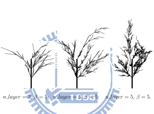
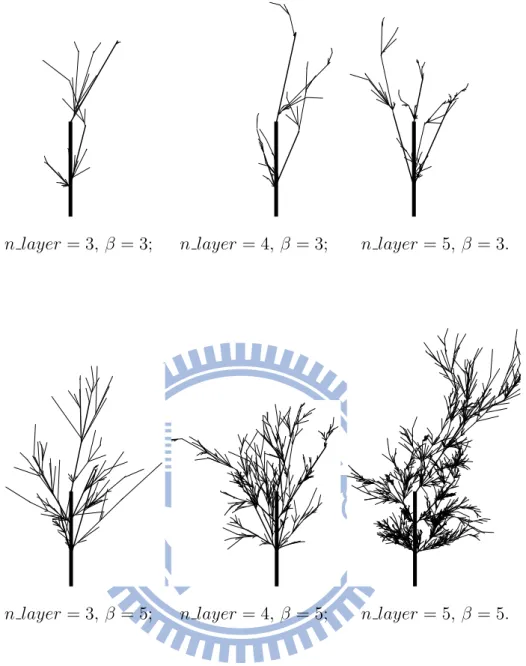
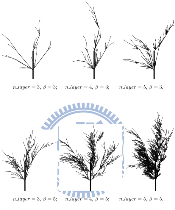
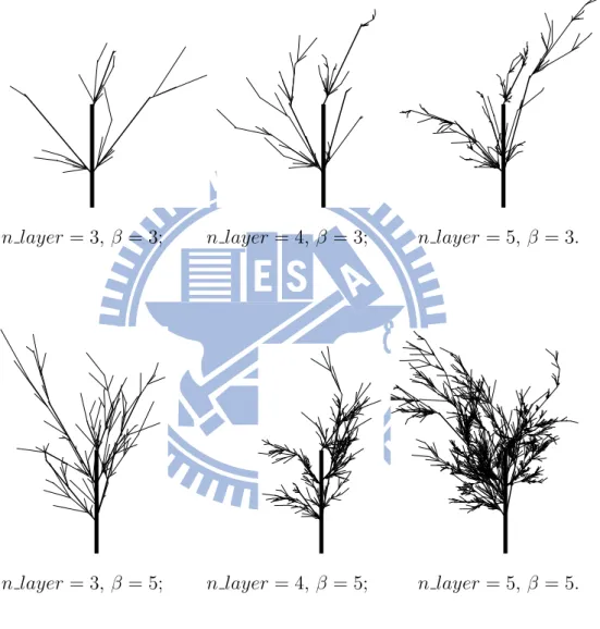
There is an infinite number of the treelike graphs in each model. In fact, each graph is unique and incomparable because it is hard to say which is lovely or not. Some of them are illustrated by the following figures.
From Figure 5.1 to Figure 5.15, there are some randomly picked results in specific condi-tions of IFS and the proposed models in the thesis. It is apparent in Figure 5.1 that the IFS
model will produce treelike images obeying their initial pattern, while the proposed models here will produced treelike images in an unrestricted way. The length and angle from hori-zontal line of each branch are randomly distributed within a range, even the bifurcation point of which is also irregular from Figure 5.2 to Figure 5.15.
Besides, Grown Tree Simulation also makes a difference to Growing Tree Simulation. From Figure 5.9 to Figure 5.15, these treelike images are denser than which from Figure 5.2
to Figure 5.8. In Growing Tree Simulation, time factor is the key distinction. Trees in the models are growing as time goes by. However, there may be too less restrictions like natural factors or human factors which also influence the form of a tree taken into consideration. So, the trees generated by the Growing Tree Simulation look so bushy.
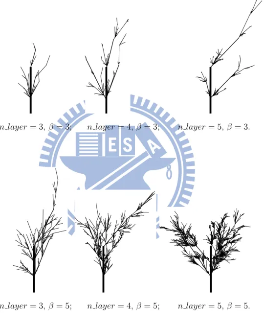
As mentioned before, equation (2.1) has chaotic behavior for 3.57 < γ ≤ 4. Thus, we pick the values 4, 3.98 and 3.8 as the LMG in Grown Tree Simulation and Growing Tree Simulation. They can be seen from Figure 5.3 to Figure 5.5 as well as from Figure 5.10 to Figur 5.12. There are no evident differences in every figure. Because they all reveal some disorder such as length and angel of branches, it is not easy to tell one from another when they have different γ. To be more objective, we will test them by hypothesis testing in the next subsection.
In equation (2.2), it has been shown when γ ≥ 4, it is uniformly distributed in the range from 0 to 1. Any γ not less than 4 can be our generator. From Figure5.6 to Figure5.8, there are three different values which are 4.1, 53 and 36.9 picked as the generator in Grown Trees Simulation. Also, the γ values of 5, 23 and 53.5 are picked as the MLMG in Grown Trees Simulation from Figure 5.13 to Figure 5.15. Generally speaking, it is hard to distinguish the results of any value of γ from the others with our eyes. In the next subsection, hypothesis testing will give one kind of interpretation about them.
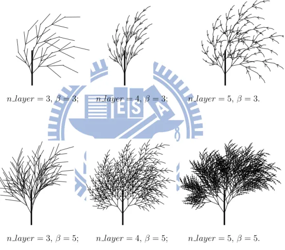
In fact, results of the Growing Tree Simulation are dynamic. The process of how a tree is growing by the model can be seen. Some of them are intercepted from Figure 5.16 to Figure 5.21. From Figure 5.16 to Figure 5.18, they are the growing processes under specific condition when the most layer is 4 and the most number of branches at a layer is 3 in Growing Tree Simulation with the three different generator individually. And from Figure 5.19 to Figure 5.21, they are under the condition when the most layer is 4 and the most number of branches at a layer is 5. So the latter will be more complicated than the former. For each Figure, from (a) to (h), the time interval between two images is fixed. It is clear that the growth rate of the tree will decrease gradually in Growing Tree Simulation because the
growing function works. Also, the upper limit of the trunk and each branch are set as well. Take the truck for example, it is growing at beginning, and it stops once it reaches its upper bound. Even these factors are taken into account, it is still insufficient for the needs to simulate a true tree in the real world. A true tree is affected by various natural and human factors, such as climate, landform, disaster and human disturbance. These variables are hard to be put in the models. However, the generators work in our models may be the best design in the aspect of it chaos.
n layer = 3, β = 3; n layer = 4, β = 3; n layer = 5, β = 3.
n layer = 3, β = 5; n layer = 4, β = 5; n layer = 5, β = 5.
n layer = 3, β = 3; n layer = 4, β = 3; n layer = 5, β = 3.
n layer = 3, β = 5; n layer = 4, β = 5; n layer = 5, β = 5.
n layer = 3, β = 3; n layer = 4, β = 3; n layer = 5, β = 3.
n layer = 3, β = 5; n layer = 4, β = 5; n layer = 5, β = 5.
n layer = 3, β = 3; n layer = 4, β = 3; n layer = 5, β = 3.
n layer = 3, β = 5; n layer = 4, β = 5; n layer = 5, β = 5.
n layer = 3, β = 3; n layer = 4, β = 3; n layer = 5, β = 3.
n layer = 3, β = 5; n layer = 4, β = 5; n layer = 5, β = 5.
n layer = 3, β = 3; n layer = 4, β = 3; n layer = 5, β = 3.
n layer = 3, β = 5; n layer = 4, β = 5; n layer = 5, β = 5.
n layer = 3, β = 3; n layer = 4, β = 3; n layer = 5, β = 3.
n layer = 3, β = 5; n layer = 4, β = 5; n layer = 5, β = 5.
n layer = 3, β = 3; n layer = 4, β = 3; n layer = 5, β = 3.
n layer = 3, β = 5; n layer = 4, β = 5; n layer = 5, β = 5.
n layer = 3, β = 3; n layer = 4, β = 3; n layer = 5, β = 3.
n layer = 3, β = 5; n layer = 4, β = 5; n layer = 5, β = 5.
n layer = 3, β = 3; n layer = 4, β = 3; n layer = 5, β = 3.
n layer = 3, β = 5; n layer = 4, β = 5; n layer = 5, β = 5.
n layer = 3, β = 3; n layer = 4, β = 3; n layer = 5, β = 3.
n layer = 3, β = 5; n layer = 4, β = 5; n layer = 5, β = 5.
n layer = 3, β = 3; n layer = 4, β = 3; n layer = 5, β = 3.
n layer = 3, β = 5; n layer = 4, β = 5; n layer = 5, β = 5.
n layer = 3, β = 3; n layer = 4, β = 3; n layer = 5, β = 3.
n layer = 3, β = 5; n layer = 4, β = 5; n layer = 5, β = 5.
n layer = 3, β = 3; n layer = 4, β = 3; n layer = 5, β = 3.
n layer = 3, β = 5; n layer = 4, β = 5; n layer = 5, β = 5.
n layer = 3, β = 3; n layer = 4, β = 3; n layer = 5, β = 3.
n layer = 3, β = 5; n layer = 4, β = 5; n layer = 5, β = 5.
(a) (b)
(c) (d)
(e) (f)
(g) (h)
n layer = 4, β = 3
(a) (b)
(c) (d)
(e) (f)
(g) (h)
n layer = 4, β = 3
(a) (b)
(c) (d)
(e) (f)
(g) (h)
n layer = 4, β = 3
(a) (b)
(c) (d)
(e) (f)
(g) (h)
n layer = 4, β = 5
(a) (b)
(c) (d)
(e) (f)
(g) (h)
n layer = 4, β = 5
(a) (b)
(c) (d)
(e) (f)
(g) (h)
n layer = 4, β = 5
5.2
Statistical Analysis
The following will introduce the use of two-sample hypothesis tests in the thesis as well as results of comparisons of the tree patterns.
5.2.1 Two-Sample Hypothesis Tests
A statistical hypothesis is an assumption about a population parameter. The most accurate method to determine whether the hypothesis is true or not is to exam the entire population. However, it is often impractical, so a random sample from the population is usually examined instead. There are four steps for testing a hypothesis in the thesis:
Step 1: State the hypotheses. This involves the null hypothesis, denoted by H0, as well as
alternative hypothesis, denoted by H1, and they are mutually exclusive.
Step 2: Choose the level of significance, denoted by α, which stands for the probability of error in making decision to reject null hypothesis.
Step 3: Compute the p-value which is the probability of rejecting a correct null hypothesis. For example, a p-value of 0.01 means there is a 1% chance that the null hypothesis is correct.
Step 4: Interpret results. If the p-value is less than α, the null hypothesis is rejected, and vice versa.
In the research, we are more interested in whether two populations have the same mean or of which mean is greater. In our case, every two samples are drawn from two independent normal populations. Also, because the variances, denoted by σ2, of the samples are unknown,
we should use F-test to test whether the two samples have equal variance first. That is, the hypothesis is stated:
• H0 : σ21 = σ22
H1 : σ21 6= σ22
The result whether the null hypothesis is rejected determine the type of t-test for two population means. In other words, we use t-test to test for µ1− µ2 then. The hypothesis can
be stated:
• H0 : µ1− µ2 ≥ δ
• H0 : µ1− µ2 = δ
H1 : µ1− µ2 6= δ
• H0 : µ1− µ2 ≤ δ
H1 : µ1− µ2 > δ
And depending on the result of F-test, the t-test will be with different kind of degree of freedom which will affect the p-value. Thus, the result of whether the null hypothesis is rejected can be concluded. Two-sample hypothesis test in our case is illustrated, one of the most significant thing is that how we take advantage of it to make good comparisons and give proper interpretations next.
5.2.2 Results of Statistical Analysis
As mentioned in sectino 4.2, these results made by programs will be transformed into sample data in order to be compared. We randomly select 100 samples in each assigned condition, and make comparisons with one another. In Figure 5.22, there are three brief illustrations of the available boundary in our sample data. Also, (a) is one example of the IFS model, (b) is one of Grown Tree Simulation and (c) is one of Growing Tree Simulation. They are selected in the part from the top to the one third of height. Then, the area coverage rate which is defined as the ratio of the number of pixels of tree image to the whole pixels in the region is obtained within the boundary. After the step for getting the sample data, these data will be analyzed by statistical hypothesis testing. We question whether these models make a deal of difference with one another or not. Moreover, we also question whether there is a big difference between the simulation and the real world. Through hypothesis testing, we set the level of significance α = 0.05 and process the data by computer. Compare the p-value which is an indicator of assessing the significance level of the result with α, the conclusion whether the null hypothesis is rejected can be obtained immediately. For clarity, they are summarized as follows.
The comparison of the value of γ among LMG in Grown Tree Simulation. As mentioned before, the selection of γ as LMG is limited. When γ = 4, equation (2.1) has chaotic behavior and its chaotic attractor is uniformly distributed in [0, 1]. Thus, γ = 4 may be the best value as LMG theoretically. However, equation (2.1) has chaotic behavior when 3.57 < γ ≤ 4. In order to know whether the different γ makes differences in Grown Tree Simulation, we have picked some values of γ in (3.57,4) to compare with γ = 4 as the LMG.
All samples are under the condition that n layer = 4 and β = 5. By two-sample hypothesis testing, the results of some cases are computed and concluded as below.
• Grown Tree Simulation with γ = 4 and γ = 3.98 LMG:
P-value. 0.11298.
Conclusion. The data don’t provide sufficient evidence to say that the means of the area coverage rate of Grown Tree Simulation with γ = 4 and γ = 3.98 LMG are not the same.
• Grown Tree Simulation with γ = 4 and γ = 3.89 LMG:
P-value. 9.6017 × 10⁻⁶.
Conclusion. The data present sufficient evidence to indicate that with α = 0.05 the mean of the area coverage rate of Grown Tree Simulation with γ = 4 LMG is smaller than γ = 3.89.
• Grown Tree Simulation with γ = 4 and γ = 3.68 LMG:
P-value. 8.7452 × 10⁻¹³.
Conclusion. The data present sufficient evidence to indicate that with α = 0.05 the mean of the area coverage rate of Grown Tree Simulation with γ = 4 LMG is smaller than γ = 3.68.
These tests show that when γ is near and smaller than 4, the mean of the area average rate may not make big difference with γ = 4. However, as the γ becomes even smaller than 4, the mean of the area average rate is more distinct and greater. By hypothesis test, these results imply that the trees are denser as the value of γ is farther from 4 and greater than 3.57.
The comparison of the value of γ among LMG in Growing Tree Simulation. In the paragraph, in order to know whether the different γ LMG makes differences in Growing Tree Simulation, we also pick some values of γ in (3.57,4) to compare with γ = 4 as the LMG. All samples are under the condition that n layer = 4 and β = 5. By two-sample hypothesis testing, the results of some cases are computed and concluded as below.
P-value. 0.47128.
Conclusion. The data don’t provide sufficient evidence to say that the means of the area coverage rate of Growing Tree Simulation with γ = 4 and γ = 3.97 LMG are not the same.
• Growing Tree Simulation with γ = 4 and γ = 3.89 LMG:
P-value. 0.026526.
Conclusion. The data present sufficient evidence to indicate that with α = 0.05 the mean of the area coverage rate of Growing Tree Simulation with γ = 4 LMG is smaller than γ = 3.89.
• Growing Tree Simulation with γ = 4 and γ = 3.6 LMG:
P-value. 2.8598 × 10⁻⁸.
Conclusion. The data present sufficient evidence to indicate that with α = 0.05 the mean of the area coverage rate of Growing Tree Simulation with γ = 4 LMG is smaller than γ = 3.6.
These tests show that when γ is near and smaller than 4, the mean of the area average rate may not make big difference with γ = 4 in Growing Tree Simulation. However, as the γ becomes even smaller than 4, the mean of the area average rate is more distinct and greater. By hypothesis test, these results also imply that the trees are denser as the value of γ is farther from 4 and greater than 3.57.
The comparison of the value of γ among MLMG in Grown Tree Simulation. In equation (2.2), we have explained that any γ ≤ 4 can be picked as MLMG. In order to know whether the different γ makes differences in Grown Tree Simulation, we have picked some values of γ > 4 as the MLMG and compare them. All samples are under the condition that n layer = 4 and β = 5. By two-sample hypothesis testing, the results of some cases are computed and concluded as below.
• Grown Tree Simulation with γ = 5.5 and γ = 15.5 MLMG:
Conclusion. The data don’t provide sufficient evidence to say that the means of the area coverage rate of Grown Tree Simulation with γ = 5.5 and γ = 15.5 MLMG are not the same.
• Grown Tree Simulation with γ = 53.3 and γ = 59.9 MLMG:
P-value. 0.92766.
Conclusion. The data don’t provide sufficient evidence to say that the means of the area coverage rate of Grown Tree Simulation with γ = 53.3 and γ = 59.9 MLMG are not the same.
• Grown Tree Simulation with γ = 5 and γ = 61 MLMG:
P-value. 0.38352.
Conclusion. The data don’t provide sufficient evidence to say that the means of the area coverage rate of Grown Tree Simulation with γ = 5 and γ = 61 MLMG are not the same.
These tests show that when γ is greater than 4, the mean of the area average rate may not make difference with one another. This implies the all results made by each γ > 4 generator reaches the same level of density or randomness in Grown Tree Simulation.
The comparison of the value of γ among MLMG in Growing Tree Simulation. Besides, we also want to know whether the different γ as the MLMG makes differences in Growing Tree Simulation, we also pick some values of γ > 4 as the MLMG and compare them. All samples are under the condition that n layer = 4 and β = 5. By two-sample hypothesis testing, the results of some cases are computed and concluded as below.
• Growing Tree Simulation with γ = 5 and γ = 53 MLMG:
P-value. 0.061057.
Conclusion. The data don’t provide sufficient evidence to say that the means of the area coverage rate of Growing Tree Simulation with γ = 5 and γ = 53 MLMG are not the same.
• Growing Tree Simulation with γ = 41 and γ = 73 MLMG:
Conclusion. The data present sufficient evidence to indicate that with α = 0.05 the mean of the area coverage rate of Growing Tree Simulation with γ = 41 MLMG is smaller than γ = 73.
• Growing Tree Simulation with γ = 4.99 and γ = 65 MLMG:
P-value. 0.33964.
Conclusion. The data present sufficient evidence to indicate that with α = 0.05 the mean of the area coverage rate of Growing Tree Simulation with γ = 4.99 MLMG is smaller than γ = 65.
These tests show that when γ is greater than 4, the mean of the area average rate may not make difference with one another. This implies the all results made by each γ > 4 generator achieves the same level of density or randomness in Growing Tree Simulation. In theory, MLM modified logistic map and extend the γ range to a value more than 4. By hypothesis test, it remains consistent in the results that MLM is chaotic with large parameter space.
The comparison among the generators in Grown Tree Simulation. There are three generators to be used in Grown Tree Simulation: PRNG, LMG as well as MLMG. In order to test the relations between two generators, all samples are set n layer = 4 and β = 5. Though varied γ in LMG will lead to different results, we pick 4 as the γ in LMG. Besides, we randomly select the value in [4,100] as the γ in MLMG to be the sample data. Thus, the three generators produce values uniformly distributed in [0,1]. By two-sample hypothesis testing, the results of the some cases are computed and concluded as below.
• Grown Tree Simulation with LMG and PRNG :
P-value. 0.0010299.
Conclusion. The data present sufficient evidence to indicate that with α = 0.05 the mean of the area coverage rate of Grown Tree Simulation with LMG is smaller than PRNG.
• Grown Tree Simulation with LMG and MLMG:
P-value. 0.026121.
Conclusion. The data present sufficient evidence to indicate that with α = 0.05 the mean of the area coverage rate of Grown Tree Simulation with LMG is smaller than MLMG.
• Grown Tree Simulation with PRNG and MLMG:
P-value. 0.11701.
Conclusion. The data don’t provide sufficient evidence to say that the means of the area coverage rate of Grown Tree Simulation with PRNG and MLMG are not the same.
The tests show under n layer = 4 and β = 5, the trees of Grown Tree Simulation with PRNG and MLMG are denser than with γ = 4 LMG. It is not easy to interpret the real reason about the results. There are two main factors affect the size of area coverage rate: length and angle of branches. We can not determine which generator possesses the highest level of randonness. Still, we could know that, in Grown Tree Simulation, the trees mady by PRNG and MLMG are denser than by LMG.
The comparison among the generators in Growing Tree Simulation. In order to test the relations between two generators in Growing Tree Simulation, all samples with different kind of generators are set n layer = 4 and β = 5. Also, we select 4 as the γ in LMG and randomly picked a value in [4,100] as the γ in MLMG. By two-sample hypothesis testing, the results of the three cases are computed and concluded as below.
• Growing Tree Simulation with LMG and PRNG:
P-value. 0.0010299.
Conclusion. The data present sufficient evidence to indicate that with α = 0.05 the mean of the area coverage rate of Growing Tree Simulation with LMG is small than with PRNG.
• Growing Tree Simulation with LMG and MLMG:
P-value. 0.026121.
Conclusion. The data present sufficient evidence to indicate that with α = 0.05 the mean of the area coverage rate of Growing Tree Simulation with LMG is small than with MLMG.
• Growing Tree Simulation with PRNG and MLMG:
Conclusion. The data don’t provide sufficient evidence to say that the means of the area coverage rate of Growing Tree Simulation with PRNG and MLMG are not the same.
We infer that the area coverage rate mean of the treelike graphs with PRNG or MLMG makes no difference to Growing Tree Simulation under the same initial condition. However, the value of area coverage rate mean of Growing Tree Simulation with LMG is tested smaller than the others. Maybe we could say that the samples of treelike graphs made by Growing Tree Simulation with LMG may be sparser than which of PRNG and MLMG.
The comparison of Grown Tree Simulation with the IFS model. There are three pairs of sample data here. The results of Grown Tree Simulation with three kinds of generators separately are compared with that of the IFS model. In order to know whether the results of these models are different from the IFS model, all samples are set n layer = 4 and β = 5, and their initial condition such as the length or the angle of the branches at the first layer are set in the same way. Besides γ = 4 is picked as LMG, and a value in [4,100] is randomly picked as MLMG. By two-sample hypothesis testing, the results of the three cases are computed and concluded as below.
• Grown Tree Simulation with PRNG and the IFS model:
P-value. 8.8607 × 10−40.
Conclusion. The data present sufficient evidence to indicate that with α = 0.05 the mean of the area coverage rate of Grown Tree Simulation with PRNG is smaller than that of the IFS model.
• Grown Tree Simulation with LMG and the IFS model:
P-value. 1.955 × 10−44.
Conclusion. The data present sufficient evidence to indicate that with α = 0.05 the mean of the area coverage rate of Grown Tree Simulation with LMG is smaller than that of the IFS model.
• Grown Tree Simulation with MLMG and the IFS model:
Conclusion. The data present sufficient evidence to indicate that with α = 0.05 the mean of the area coverage rate of Grown Tree Simulation with MLMG is smaller than that of the IFS model.
Every p-value here is much smaller than 0.01 and it means that these result of every pro-posed model here is almost certainly smaller than which of IFS model. It implies that Grown Tree Simulation and IFS model really show a sharp distinction in their level of denseness and appearance of the treelike graphs in the aspect of area coverage rate.
The comparison of each model with natural trees. There are seven pairs of sample data here. The results of all models in the thesis are compared with trees in the nature world. In order to test whether the results of these models are equal to trees in the real world or not, we have to find applicable samples in the nature world first. As shown in Figure 5.23, there are some photos of the selected tree group. Then we also decide the boundary of every photo (Figure 5.24) and transform it into one of the sample data. On the other hand, all other graphs made by our models and IFS model are set n layer = 4 and β = 5. The γ of LM is set 4, and which of MLM is randomly set in [4,100]. Besides, we should plot leaves on them and set their boundary as shown in Figure 5.25 and Figure 5.26. By two-sample hypothesis testing, the results of these cases are computed and concluded as below.
• The IFS model and a tree group in the world:
P-value. 0.494337.
Conclusion. The data present sufficient evidence to indicate that with α = 0.05 the mean of the area coverage rate of the IFS model is smaller than that of tree group in the selected region.
• Grown Tree Simulation with PRNG and a tree group in the world:
P-value. 1.06times10−9.
Conclusion. The data present sufficient evidence to indicate that with α = 0.05 the mean of the area coverage rate of Grown Tree Simulation with PRNG is smaller than that of tree group in the selected region.
• Grown Tree Simulation with LMG and a tree group in the world:
Conclusion. The data present sufficient evidence to indicate that with α = 0.05 the mean of the area coverage rate of Grown Tree Simulation with LMG is smaller than that of tree group in the selected region.
• Grown Tree Simulation with MLMG and a tree group in the world:
P-value. 8.9462 × 10⁻¹⁰.
Conclusion. The data present sufficient evidence to indicate that with α = 0.05 the mean of the area coverage rate of Grown Tree Simulation with MLMG is smaller than that of tree group in the selected region.
• Growing Tree Simulation with PRNG and a tree group in the world:
P-value. 5.1629 × 10⁻⁵.
Conclusion. The data present sufficient evidence to indicate that with α = 0.05 the mean of the area coverage rate of Growing Tree Simulation with PRNG is greater than that of tree group in the selected region.
• Growing Tree Simulation with LMG and a tree group in the world:
P-value. 0.0019258.
Conclusion. The data present sufficient evidence to indicate that with α = 0.05 the mean of the area coverage rate of Growing Tree Simulation with LMG is greater than that of tree group in the selected region.
• Growing Tree Simulation with MLMG and a tree group in the world:
P-value. 0.00031078.
Conclusion. The data present sufficient evidence to indicate that with α = 0.05 the mean of the area coverage rate of Growing Tree Simulation with MLMG is greater than that of tree group in the selected region.
There are some limits in the comparison by nature. The treelike graphs are two dimension figures, while the trees in the real world are growing in three dimension space in nature. Even the photos of real trees we take are two dimension figures as well, there are still more complex perspectives than our simulation. Obviously, the truck and the branches made by these models are linear, and the leaves are plotted on every end of the branches. They are different from the trees in the real world. However, there are still some suggestions in the case by the
hypothesis test. From the results, we infer that the denseness of trees made by IFS model is closer to the tree group we choose than Growing Tree Simulation as well as Grown Tree Simulation when n layer = 4 and β = 5. However, the results of Growing Tree Simulation and the tree group are acceptable. As mentioned earlier, some factors are not taken into account like natural disasters in Growing Tree Simulation. Namely, it is growing under a near-perfect condition without any interference and destruction. In this way, it is expected that the density of Growing Tree Simulation is larger than the trees in the real world. Besides, the level of denseness can be inferred here, the most one is Growing Tree Simulation, the second one is IFS model and Grown Tree Simulation is the last.
(a) (b) (c)
n layer = 4, β = 5
(a)
(b)
(c)
(a)
(b)
(c)
n layer = 4, β = 5
(a)
(b)
(c)
n layer = 4, β = 5
5.3
Summary
Because of two-sample hypothesis tests used here, these results produced by the proposed models can be compared in a well-founded way. The p-value of every case may be a little alterant if other 100 sample data are chosen. Also, the probability that null hypothesis is inappropriately rejected increases if α increases. That is, the smaller α will minimize errors of decision. That seems so uncertain in the statistical analysis. However, these conclusions of the tests still provide convincing views on how to interpret these tree patterns made by the models.
The logistic map with different γ will affect the results. Generally, as the γ increases in (3.57,4), the value of area coverage rate is decreasing. Because the sequence of logistic map will distribute over 0 to 1 when γ approach 4 and they will reach higher level of randomness. However, modified logistic map has more range of γ available here, the γ can be any value larger than 4 and their results will reach same level of denseness.
Also, we can infer that IFS model and Grown Tree Simulation even under same initial condition still have distinct results in a way. Owing to the destruction of self-similarity of IFS models, the latter is not as ordered as the former. Thus, area coverage rate of Grown Tree Simulation is smaller than which of IFS models. Instead, the tree patterns of the same simulation with the different generators make less differences. They are roughly concluded that tree patterns simulated with random or modified logistic map are denser than with logistic map.
In the end, the models can be compared with trees in the real world. It is surprising that these treelike graphs may be closer to the trees in the world than what we think. From the hypothesis tests, we finally classify the denseness of these tree patterns according to size. Growing Tree Simulation ranks the first; the trees in the real world is in second spot; IFS model is the third; Growing Tree Simulation is the last one. Owing to the natural or man-made factors are taken into considerations, it can be reasonable that the density of Growing Tree Simulation is larger than the trees in the real world.
However, it has no absolute solution which model is better here because each of them, through some modifying, probably becomes a near-perfect simulation of the trees belonging to a specific tree group some day.
6
Conclusions and Future Works
In this thesis, random and chaotic sequences are used to simulate the tree patterns rather than the common fractal trees. We incline to query whether random and chaotic sequences differ from each other. Instead of analyzing them directly, we focus on the comparison of their visualization. By hypothesis tests, the treelike results produced by the three generators can be compared in a convincing way. In the end, the conclusion that tree patterns simulated by logistic map generators are sparser than by pseudorandom number generator and modified logistic map generator is inferred from the hypothesis tests. Though the appearances of these trees made by different generators are difficult to recognize immediately, random and chaotic sequences seem to take on another interesting aspect through the visualization.
Besides, breaking the self-similarity of the fractal trees, our proposed models can display various types of treelike results. This thesis also gives a further study on the difference between the simulation and the real world. This conclusion may be amazing that the indicator, area coverage rate, we define of the modeled tree patterns can be compared with which of the real ones and interpreted in a rational way.
At current stage, these tree pattern are simulated as two-dimension images. It would be practical if they can be modeled under three-dimension or nonlinear conditions. On the other hand, if the growing function can be aimed at the appointed tree group whose growing con-ditions such as natural or man-made factors are taken into account as well, these simulations may get even closer to the real world.
References
[1] Michael F. Barnsley. Lecture notes on iterated function systems. In Chaos and Fractals: The Mathematics Behind the Computer Graphics, pages 127–144, 1988.
[2] Michael Batty and Paul Longley. Fractal Cities: A Geometry of Form and Function. Academic Press, London, 1994.
[3] John Briggs. Fractals: The Pattern of Chaos. Simon and Schuster, New York, 1992.
[4] Shu-Ming Chang, Ming-Chia Li, and Wen-Wei Lin. Asymptotic synchronization of mod-ified logistic hyper-chaotic systems and its applications. Nonlinear Analysis: Real World Applications, 10:869–880, 2009.
[5] Ming-Jang Chen. http://web2.cc.nctu.edu.tw/ mjchen/.
[6] Shih-Liang Chen, Shu-Ming Chang, Wen-Wei Lin, and Ting-Ting Hwang. Digital secure-communication using robust hyper-chaotic systems. Int. J. Bifurcation Chaos, 18(11):3325–3339, 2008.
[7] Robert L. Devaney. Chaotic bursts in complex dynamical systems. In Applications of Fractals and Chaos, pages 195–206, 1993.
[8] Gary William Flake. The Computational Beauty of Nature: Computer Explorations of Fractals, Chaos, Complex Systems, and Adaptation. The MIT Press, Cambridge, Massachusetts, 1998.
[9] John Mordechai Gottman, James D. Murray, Catherine C. Swanson, Rebecca Tyson, and Kristin R. Swanson. The Mathematics of Marriage: Dynamic Nonlinear Models. Mit Pr, 2005.
[10] Hans Lauwerier. Fractal: Endless Repeated Geometrical Figures. Princeton University Press, New Jersey, 1991.
[11] Blake LeBaron. Chaos and nonlinear forecastability in economics and finance. In Chaos and Forecasting: Proceedings of the Royal Society Discussion Meeting, pages 129–143, 1994.
[12] Mario Livio. The Golden Ratio. Random House, Inc., 2002.
[14] Benoit B. Mandelbrot. Fractal geometry: What is it, and what does it do? In Fractals in the Natural Sciences, pages 3–16, 1988.
[15] George Marsaglia. Random numbers fall mainly in the planes. Proceedings of the National Academy of Sciences, 61:25–28, 1968.
[16] Robert M. May. Simple mathematical models with very complicated dynamics. Nature, 261:459–467, June 1976.
[17] Michael McGuire. An Eye for Fractals: A Graphic and Photographic essay. Addison-Wesley, 1991.
[18] Cleve B. Moler. Numerical Computing with MATLAB. SIAM, 2004.
[19] Andrew Rukhin, Juan Soto, James Nechvatal, Miles smid, Elaine Barker, Stefan Leigh, Mark Levenson, Mark Vangel, David Banks, Alan Heckert, James Dray, and San Vo. A statistical test suite for the validation of random number generators and pseudo random number generators for cryptographic applications. NIST, National Institite of Standards and Technology, (SP 800-22 Rev. 1a), Apr. 2010.
[20] Julien Clinton Sprott. Chaos and time-series analysis. Oxford University Press Inc., New York, 2003.
[21] Anastasios A. Tsonis. Chaos: From Theory to Applications. Plenum Press, New York, 1992.