基於正交分頻多重進接之無線多媒體傳收機研究及設計---子計畫V：適應性編碼調變及頻寬管理(I)

行政院國家科學委員會專題研究計畫 期中進度報告

子計畫五:適應性編碼調變及頻寬管理(1/2)

計畫類別： 整合型計畫

計畫編號： NSC92-2219-E-009-019-

執行期間： 92 年 08 月 01 日至 93 年 07 月 31 日

執行單位： 國立交通大學電信工程研究所

計畫主持人： 張文鐘

報告類型： 完整報告

報告附件： 出席國際會議研究心得報告及發表論文

處理方式： 本計畫可公開查詢

中 華 民 國 93 年 10 月 4 日

基於正交分頻多重進接之無線電多媒體傳收機研究及設計(子計畫5)

適應性編碼調變及頻寬管理(1/2)

Adaptive coded modulation and bandwidth management

計畫編號：NSC 92-2219-E-009-019 執行期限：92 年 08 月 01 日至 93 年 07 月 31 日 主持人：張文鐘 交通大學電信系 E-mail:wtchang@cc.nctu.edu.tw 一,中文摘要 可調式調變是根據瞬間訊雜比來決定調變模 式。在單一載波時，一般我們常用 Torrance 及 Lagrange 方法來求所需的改變臨界值。臨 界值是根據位元錯誤率及傳送率之間的比較 而決定。這兩個方法都把通道變化描述成一個 SNR 數學式，再由 Cost Function 來決定臨界 值。本研究探討如何簡化 Torrance 的求解方 法。我們首先提出漸近式的求解法，先從最低 的二個模式的臨界值開始求（把其它值設為無 窮大）。當最低的值找出之後，再找第二個臨 界值。這個值一定是在第一個值跟無窮大之 間。因此，一個值的變化，只跟二個相關的調 變模式有關。由這個道理，我們繼續簡化求解 公式，而提出了單一模式的調變成本函數。利 用這些單一模式的調變成本來決定臨界值。最 後再把單一載波所求到的臨界值應用到多載 波之情況。

Abstract- In single carrier, the two formulations

that are commonly used in the determination of the switching levels are the Torrance cost function and the Lagrangian optimization. From the Lagrangian optimization, it can be seen that the switching levels can be each separately related to the target bit error rate with the constraint that the average bit error satisfies the target bit error requirement. This provides a search direction for the optimum solution of the Torrance formulation. In this case, each switching level is only related to two adjacent modulation modes. Based on this relation, we approximate the Torrance formulation with a two-mode one-dimensional search problem. From this decomposition, we further develop a one mode cost function to derive the switching level. This method evaluates the cost of using one specific modulation mode as a function of instantaneous SNR. Switching levels can be determined by simply comparing these one mode cost function. We then evaluate these switching levels at the case of multi-carrier and try to find a way to represent the mean SNR for the case of multi-carrier.

二,緣由與目的

In adaptive modulation, the aim is to optimize the set of switching levels s, so that the average BPS throughput

B r s

( , )

can be maximized under the constraint

P

_avg

( ; )

r s

=

P

_th, where

avg

P

for a K-mode adaptive coded modulation scheme is defined as the sum of the mode specific average BEP weighted by the BPS throughput of the individual constituent mode (bit error per symbol) divided by the average BPS (bit per symbol):

1 0 1 0

( ; )

1

K R k k k K avg k k k

P r s

b P

P

b P

B

− = − =

=

∑

∑

@

(1)

and

P

_th is the target bit error threshold,

r

is the average SNR per symbol, s is the set of switching levels, K is the number of constituent coded-modulation modes,

b

_k is the BPS throughput of the k-th constituent mode and the mode-specific average BEP

P

_k is given as:

1

( ) ( )

k k k s k m s

P

p

r f r dr

+

=

_∫

and the average BPS is defined as

1 1 0

( ; )

( ; )

k k s K k k s

B r s

b

f r r dr

+ − =

=

∑ ∫

(2) Two of the popular methods that are used to derive the switching levels are the Torrance method and the Lagrangian method [1][2][3][4]. The Torrance cost function is defined as

10 max

( ; ) 10 log (max{

( ; ) /

,1})

( ; )

avg th avg

s r

P

r s

P

B

B

r s

Ω

=

+

−

while the Lagrange method define the cost function as

{

}

( ; )

( ; )

( ; )

( ; )

=(1-

) ( ; )

( ; )

R th th R

s r

B r s

P r s

P B r s

P B r s

P r s

λ

λ

λ

Λ

=

+

−

+

The difference between these two formulations is the way to express the relation between

P

_avg and

P

_th . Although it is formulated as a multidimensional search problem in the Torrance formulation, actually, the switching

levels can be derived as a function of the

P

_th only. This fact is indicated by the solution derived from the Lagrange method.

The Lagrange cost function can be evaluated as:

{

}

(

)

(

)

{

1 1

}

( ; )

( ; )

( ; )

0

1

( )

( )

( ) 0

k k R th k th k m k k m k k

B r s

P r s P B r s

s

s

c

P

b p

s

b p s

f s

λ

λ

λ

− ₋

∂Λ ∂

₌

₊

₋

₌

∂ ∂



_{− −}

₊

₋



₌





When

f s

( )

_k

≠

0

, it can be simplified by dividing both sides by

f s

( )

_k , to yield

{

1 1

}

(1

)

( )

( )

0

k k k th k m k k m k

c

λ

P

λ

b p

s

b p

s

− −

−

−

+

−

=

Re-arrange the above equation and assume

0

k

c

≠

, we have:

{

1 1

}

1

( )

( )

k k th k m k k m k k

P

b p

s

b

p

s

c

λ

λ

− ₋

−

=

−

It can be seen that the switching level s is just a function of the target bit error rate, as long as the value of

λ

is known. The following set of functions defines the relation between the switching level and the mode specific BEP.

{

1 1

}

1

( )

( )

( )

k k k k k m k k m k k

y s

b p

s

b

p

s

c

−

− −

@

(3)

The set of switching level needs to satisfy the constraint function

Y r s s

( , ( ))

k defined as

( , ( ))

_{k R}

( , ( ))

_{k th}

( , ( ))

_k

Y r s s

@

P r s s

−

P B r s s

(4) Eq(3) indicates that each of the switching levels can be separately derived but is a function of

1

−

λ

P

_th, as long as the set of switching level satisfies the requirement of the Y function in Eq(4). For the case if the requirement can not be met, such as in a low average SNR channel, we will have to use the Torrance constraint. In this case, assume that there is no

P

_th in the formulation. From the Lagrange solution, it is seen that the optimum solution of the switching level is only related to two adjacent modes. The consideration of

P

_th makes the Torrance formulation non-linear. If

P

_this removed, the formulation is a linear and each switching level can be independently derived. A solution for this case with SNR=25 db is shown in Table 1. 三、研究方法及成果

Based on this argument, a successive optimization method is proposed in this paper. This method finds the solution from the first threshold that the system switches from no-transmission to the first transmission mode, and successively finds the next threshold up to the highest transmission mode. During the

successive optimization, the cost function in (1) considers two modes at a time.

Since our interest is not the actual cost function, but the switching level for the available transmission modes. Or more importantly, for a particular SNR value, we compare the use of two adjacent transmission modes. We seek the mode that will result in lower cost function. So we need only to compare the part of the cost function that is affected by the use of two adjacent modes at some particular SNR. For each particular SNR value, two modes can be chosen. The objective is to choose the one that has lower total cost function.

From this two-mode cost function, we develop a simple comparison method to evaluate the cost associated with each of the transmission mode. We break the cost function that involves only two adjacent transmission modes into two separate partial cost functions. During the successive optimization, only the partial cost function is required. The partial cost function is a measure of only the part of the cost that involves with transmission mode that has been used from 0db up to a given SNR. The partial cost function associated with one particular mode up to instantaneous SNR

ξ

is derived below. Let us temporarily neglect the BER threshold by assuming that it is small enough that the system can not achieve. Also, for simplicity, the log function is neglected temporarily. Thus this derivation is not complete but an intermediate step for the setup of the following cost function that is to be proposed. Take BPSK and QPSK as an example.

1 1 1 1 1 1 1 1 1 1 0 max ₀ max 0 0 0 0 0 0

(

( ) ( , )

( ) ( , ) )

(

1 ( , )

2 ( , ) )

(

( ) ( , )

( )

( ) ( , ) ) (

1 ( , )

2

2 ( , ) )

(

( ) ( , )

1 ( , ) )

(

( ) ( , )

x B _x Q x x x x B Q Q x x x x B Q

P r f r r dr

P r f r r dr

B

f r r dr

f r r dr

P r f r r dr P r

P r f r r dr

B

f r r dr

f r r dr

P r f r r dr

f r r dr

P r f r r

∞ ∞

+

+

−

−

=

+

−

+

−

− +

=

−

−

∫

∫

∫

∫

∫

∫

∫

∫

∫

∫

1 1 0 0

2 ( , ) )

x x

dr

−

f r r dr C

+

∫

∫

0

( )

( ) ( , )

Q Q

P r

=

∫

∞

P r f r r dr

max

( )

2

Q

C

=

P r

+

B

−

The meaning of the above cost function is that when x increases, the part associated with BPSK will increase and the part associated with QPSK

will decrease. The cost function adds the amount that is to be increased and subtracts the amount that is to be removed. Based on the above derivation, we define the partial cost function as

1 1

1, _{0 0}

(

)

x _i

( ) ( , )

x

( , )

)

C x r

=

∫

P r f r r dr

−

i

∫

f r r dr

The original cost function becomes the comparison of the two partial cost functions. Both the two functions keep increase in BER as a function of x. But one is to be added and one is to be removed. The optimum solution is when the two cost functions are equal.

To make the partial cost function a monotonically decreasing function of the SNR, we normalize the cost function with the integration interval. For practical application, we also consider the BER threshold. The normalization is as follows, 1 1 1 1 1 0 0 0 0 0

(

( ) ( , )

( , )

)

( , )

( , )

( )

( , )

x x i x x x i

P r f r r dr

i

f r r dr

f r r dr

f r r

P r

dr

i

f r r dr

−

=

−

∫

∫

∫

∫

∫

For computational purpose, we modify the new normalized cost function as

1 1 0 0 10

( , )

( )

( , )

10log max(

,1)

x x i th

f r r

P r

dr

f r r dr

i

P

ρ

−

∫

∫

where

ρ

is a normalization constant. We normalize the accumulated BER by the probability interval. This will not change the final result, because both the partial cost functions are normalized by the same interval. The computation is based on the comparison of the BER value of two adjacent modulation modes. The threshold is likewise normalized by

ρ

, so the normalized BER is compared with the normalized threshold. The normalization interval is a function of the SNR.

When compared with the case derived by the peak bit error rate, it can be seen that in order to increase the throughput, the system derived from the above cost function will switch to the next higher transmission mode at a lower SNR. That is the required SNR for the change to the next higher transmission mode will be lower than that obtained by the peak bit error rate. This decrease of the threshold is at the price of larger bit error rate. But the increased bit error rate is compensated by the increased throughput. So the new switching threshold is at the point where the increased bit error rate is at equilibrium with the

increased throughput. This is the minimum point in the two-mode cost function.

A property of the cost function is that when the SNR is low, the bit error rate dominates the cost function. This part of the cost function is very similar to the bit error rate verse SNR curve. But when the SNR reaches a certain value, the bit error rate decreases to the level set by the threshold, and from that on the bit error rate is no more considered in the cost function and the throughput dominates the cost function. So an almost flat curve in the tail of the cost function results.

As explained above, the cost function is to be minimized and the switching point is where these two partial cost functions equal. The first threshold is the intersection of the cost associated with BPSK transmission mode with that of the no-transmission. In this derivation of the switching level, for any SNR, only two choices have to be made, the original transmission mode or the next higher transmission mode. Thus, the threshold is the intersection of two cost functions associated with two adjacent modes. For each used transmission mode, when the SNR increases to a certain value, the bit error rate decrease to a point where the throughput will begin to dominate. After this point, higher transmission mode will be chosen due to higher throughput.

四、結論

First let us examine the case with no

P

_th in the Torrance formulation. The optimum solution with SNR=25db is shown in Table 1 labeled as Torrance-WT. When

P

_this not considered, each switching level is related only to two adjacent transmission modes. The best achievable BER is

2.17 *10

−4. The x symbol in the column of s1 means no solution. Because without a threshold, no-transmission dominates the error rate. If

P

_th

=

10

−3is set, then there are infinite sets of solution that can achieve this BER requirement. Any switching levels can be shifted to left, as long as the requirement is kept. For the optimum solution, a full multidimensional search is then performed. The one that minimizes the cost function is listed in Table 1. In this case, the switching level is shifted to the left for higher throughput. The throughput increases from 4.5172 to 5.0193 and the BER is

7.86 *10

−4. The bit error rate and throughput for these various switching levels are listed in Table 2.

In the case of two-mode cost function, the determination of each threshold is concerned with only two adjacent modulation modes. This simplifies the search at the price of slightly reduced throughput, from 5.0193 to 4.97. For any adjacent two modes, it is the comparison of the corresponding BER and the throughput when adjusting the switching level. In the case of two modes, when one threshold is determined, the following thresholds for higher mode transition will not have any effect on it, since each threshold is only related to two adjacent transmission modes. The result shown in Fig.1 is with SNR=25db and

p

_th

=

10

−3. The result shown in Fig. 2 is with SNR=25db and

p

_th

=

10

−2. In the latter case, both s1 and s2 are zero. This is due to the low requirement of the BER as compared with the case in Fig. 1. The characteristics of the Torrance cost function is that when a switching level results in a BER that is below the threshold only the throughput is taken into account in the cost function. Starting the switching level from -∞db means the system uses the higher mode at first. As shown in Fig. 1, the value of the cost function decreases first when switching level increases from -∞db. The decrease means using lower mode will reduce the BER more than the sacrifice of the throughput. When the switching level increases, the part of the cost function involving BER will decrease. The lowest point is the switching point as shown in the red curve and the green curve in Fig.1. In the case when

p

_avg is always less than

p

_th, the minimum point is the point where decrease of BER is less than the value of the throughput reduction. From that on, the cost begins to increase.

When we set a threshold, as long as the BER reaches the threshold, the BER is no more considered. After this point, we will only see the reduction of throughput and thus the increase of cost function. This can be seen in the blue curve in Fig.1 as well as the blue curve and the green curve in Fig.2. In Fig.1, in the lowest point, the cost function has a value of 4.1 with switching level at 2db. In Fig. 2, the lowest cost is 4 for the blue curve and 2 for the green curve. This is the lowest available. This is because the low BER threshold, switching at -∞db to run the higher modulation mode will satisfy the BER requirement and result in more throughput. As long as the BER reaches the threshold, the switching point is determined. From that on, the adaptive system chooses higher transmission mode. On the other hand, the result shown in Fig.3 indicates that no switching levels will

satisfy the BER requirement due to lower SNR at 20db. In this case, the cost function is not affected by the threshold

p

th

10

3

−

=

, which is not attainable

.

The BER of higher modulation mode is always larger than the lower one. So if we compare the BER it is always the lower one that will be chosen. The comparison is thus the compensated BER with the throughput. If increasing the throughout one bit can be made to be equivalent to a certain amount of BER increase, then modulation mode can be changed. So the cost function is a measure of the value of one bit in throughput and the value of BER. Starting from the lowest mode, when the BER difference of two adjacent modes becomes smaller than the value of one bit in throughput, we change the mode. The cost function considers the difference of the two accumulations. The difference is the increase of the BER when switching from the lower mode to the higher mode.

Now let us investigate the behavior of the proposed modified cost function involving only one mode. The result with the proposed cost function is shown in Fig. 4. The appearance of the cost function is similar to the bit error rate curve. The difference is that there is a turning point specified by the target bit error rate. As shown in Fig. 4, the turning point is where the BER has reached the threshold. The intersect point between two curves is where the switching level is. As explained above, the switching point is set when the two partial cost functions equal. On the left side of the switching point, the part in the cost function associated with the lower mode is less than the part associated with the higher mode, so the cost function keeps decreasing. On the right side of the switching point, the part associated with the high mode becomes smaller, so the cost function begins to increase. The intersect point is the minimum point in the cost function. According to the y function in (3), the worth of one bit in throughput is not a constant, it depends on where the BER threshold is set. Thus the distance between the turning point and the intersect point is a function of the BER threshold. The movement of the switching level from the turning point to the intersect point is indication of the tradeoff for throughput at the price of BER. The amount of the movement depends on the worth of one bit in throughput. Our proposed method is a non-linear approximation to the original Torrance method. The accuracy of our method depends on the setting of the normalization constant

ρ

. This is done by iteratively solve the Lagrangian

constraint. In this case, s1 is tried iteratively (everything is related to s1). After the s1 is determined, we can backward to derive the normalization constant

ρ

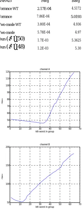
in our simplified method. The other way is to set the value based on the solution obtained either by the Torrance method or the two-mode method. The various switching levels derived from the Torrance method, two-mode method and our simplified method are listed in Table 1 for comparison. The throughput in our method is higher than that from Torrance method. The reason is due to that the s4 is 22 in Torrance method [4]. This can be due to the problem in the full search with the Matlab package. We will continue to verify this numerical problem. The above derivation is aimed at single carrier system at narrow band channel. For wide band channel and multicarrier system, still more work is needed.

In the case of single carrier, the SNR is well defined. For the case of multicarrier, we then need more complicated methods to define the SNR for a group of subcarriers, since each subcarrier in a group has its own SNR associated with it. To allow each subcarrier to adapt independently is not an economic approach. For group adaptation, we have examined several methods. The easiest one is to select the lowest SNR. It can be expected that the performance of this method is low BEP and low BPS. And the performance gets worse when the group becomes larger, since more subcarriers with good SNR have to be sacrificed. The group size actually is a function of the channel condition, because the best condition is that all the subcarriers in a group experience the same channel condition. That is all the subcarriers are within the coherent bandwidth. However, in the practical application the group size is usually fixed. This represents a problem. Another problem is that in the 802.16 OFDMA, the subcarriers are spread out uniformly distributed across the spectrum, so all the subcarriers will experience different channel condition. This is good for channel diversity but is bad for adaptive modulation. In the following, two simulations with group consisting of continuous subcarriers are shown. The purpose is to show how to select the best subcarrier to represent the group. Both simulations show the value of Torrance cost function of the adaptive system as a function of the group SNR. The cost function is defined as the sum of log of the bit error rate and the throughput for all the subcarriers in the group. In this case, the SNR of one particular subcarrier is chosen as the group SNR. The chart indicates the best subcarrier to choose to represent the group. With proper setting of the group SNR, the whole group will operate at a

more suitable transmission mode. Thus the overall error rate will be low while the throughput can be high to obtain the lowest cost function. This choice actually depends on the channel condition and the group size. In the following year, group based OFDM adaptive modulation will be investigated more for the issue of group size, group SNR definition, group with non-continuous subcarriers, etc..

References

[1] B. J. Choi and L. Hanzo, “Optimum mode switching levels for adaptive modulation systems”, IEEE GLOBECOM 2001

[2] J. Torrance and L. Hanzo, “Optimization of switching levels for adaptive modulation in a slow Rayleigh fading channel”, Electronics Letters, vol. 32, pp 1167-1169, 20 June 1996

[3] A. Goldsmith and S. Chua, “Variable rate variable power MQAM for fading channels”, IEEE Transactions on Communications, vol. 45, pp. 1219-1230, October 1997. [4] L. Hanzo, C. H. Wong and M. S. Yee “Adaptive Wireless Transceivers” Wiley 2002.

Fig1. Two mode cost function SNR=25dB ; Pth=10^-3

Fig3 Two mode cost function SNR=20dB; Pth=10^-3 ;

Fig4. Cost function for each single mode (

ρ

=

50,

P

_th

=

10 ^ 3

−

,SNR=25) Table 1a switching level with 3 methods; Pth=10^-3 ;

SNR=25 s1 s2 s3 s4 Torrance WT X 9 18 24 Torrance -∞ -2 15 22 Two-mode WT X 11 16 22 Two-mode -∞ 2 16 22 Ours

(

ρ

=

50)

_{7 9 14 19} Ours(

(

ρ

=

48)

_{8 9.2 14.2 19.5} WT—without threshold

Table 1b switching level with 3 methods; Pth=10^-3

SNR=20 s1 s2 s3 S4 Torrance 0 7 15 22 Two-mode -∞ 9 15 19 Ours

(

ρ

=

50)

_{8 9 14 21} Table 1c switching level with 3 methods; Pth=10^-3

SNR=15 s1 s2 s3 s4

Torrance 3 6 15 22

Two-mode 3 8 13 16

Ours

(

ρ

=

50)

_{8 10 15 X}

Table 2 bit error rate and throughput: Pth=10^-3 ;

SNR=25 Pavg Bavg Torrance WT 2.17E-04 4.5172 Torrance 7.86E-04 5.0193 Two-mode WT 3.80E-04 4.936 Two-mode 5.78E-04 4.97 Ours

(

ρ

=

50)

_{1.7E-03 5.3625} Ours

(

ρ

=

48)

_{1.2E-03 5.30} 0 10 20 30 40 50 60 70 40 50 60 70 80 90 100 110 120 channel A kth worst in group c o st 0 10 20 30 40 50 60 70 50 100 150 200 channel B kth worst in group c o st