應用於H.264/AVC高解析度即時系統之邊緣基底快速內部預測模組決策演算法的改善與實作

國 立 交 通 大 學

電機學院通訊與網路科技產業研發碩士班

碩 士 論 文

應用於H.264/AVC高解析度即時系統之邊緣基底快速

內部預測模組決策演算法的改善與實作

Modification

and

Implementation

of

an

Edge-Based

Fast

Intra

Prediction Mode Decision Algorithm for H.264/AVC High

Resolution Real-time Systems

研 究 生：吳明鋒

指導教授：單智君

博士

應用於H.264/AVC高解析度即時系統之邊緣基底快速內部預測模組

決策演算法的改善與實作

Modification

and

Implementation

of

an

Edge-Based

Fast

Intra

Prediction Mode Decision Algorithm for H.264/AVC High

Resolution Real-time Systems

研 究 生：吳明鋒 Student：Ming Feng Wu

指導教授：單智君 博士 Advisor：Dr.Jean Jyh-Jiun Shann 闕河鳴 博士 Dr.Her-MingChiueh

國 立 交 通 大 學

電機學院通訊與網路科技產業研發碩士班

碩 士 論 文

A Thesis

Submitted toCollege of Electrical and Computer Engineering National Chiao Tung University

in partial Fulfillment of the Requirements for the Degree of

Master in

Industrial Technology R & D Master Program on Communication Engineering

Nov.2007

Hsinchu, Taiwan, Republic of China

應用於 H.264/AVC 高解析度即時系統之邊緣基底快速內部預測模

組決策演算法的改善與實作

研究生：吳明鋒

指導教授：單智君 博士

闕河鳴 博士

國立交通大學

電機學院產業研發碩士班

摘要

本論文中提出了於H.264/AVC在高解析度即時應用時，快速內部預測模

組決策(Fast intra prediction mode decision) 的硬體架構。

由於在H.264/AVC中，內部預測模組決策的運算在整個 H.264/AVC運算

裡佔有一定比重，此外，內部預測模組決策又需要額外的時間(約20%)來產

生預測模組，加上處理資料本身又具高相 關性，因此，使得在高解析度即時

應用下出現了瓶頸。

在加速內部預測模組決策的運算中，我們使用了一種以影像邊緣資訊為

依據的演算法，能夠在不大量損失影像品質及增加傳輸資料的前提下，節省

大約66%的模組評估運算，根據此種演算法，我們提出一種硬體代價較低的

架構，相較以往的設計可以減少 約50%的邏輯閘數 ，總邏輯閘 數也僅需

86,671，最大操作頻率達到250MHz，對於目前所有高解析度影像的即時處

理有很大的效益，同時亦不用增加太多的硬體需求。

Modification and Implementation of an Edge-Based Fast

Intra

Prediction

Mode

Decision

Algorithm

for

H.264/AVC

High Resolution Real-time Systems

Student：

Wu-Ming Feng

Advisor：Dr. Jean Jyh-Jiun Shann

Dr. Her-Ming Chiueh

Industrial Technology R & D Master Program of

Electrical and Compute r Engineering College

National Chiao Tung University

ABSTRACT

In this thesis, we propose architecture of H.264/AVC fast intra

prediction mode decision in high resolution real -time applications.

Because the intra prediction mode decision occupied lots compu tations

of the H.264/AVC video coding, besides it needs the extra time for modes

generating of the intra prediction mode decision (about 20%), and the

processed data is high dependence also, hence, it is a bottleneck of the high

resolution real-time applications.

In the intra prediction mode decision operations, we use an algorithm

which based on the edge information of the object. It can reduce about 66%

estimations of mode predictions with negligible loss of video quality and a

little increasing of data rate. According to this algorithm, we propose a low

cost architecture and the gate counts can be reduced about 50% to compare

with the former design. The total gate counts are 86 ,671 only and the

maximum operating frequency is 250 MHz. It is a favorable c ontribution to

all the current high resolution real -time video processing while without

spending a lot of hardware.

誌

謝

感謝 單智君教授及闕河鳴教授在研究所求學的過程裡對我耐心的指導

以及給予的寶貴意見，使得研究得以順利完成。

此外，也感謝參予RH組討論的華鼎學長、群旻學長、奕雄同學、泰霖同

學、毓宏學弟、建辰學弟及俊賓學弟，對我研究所提出的指教及生活上給予

的幫助。

謹以此文獻給我的朋友們。

Contents

Chinese abstract i

Abstract ii

Acknowledgement iii

Contents v

List of tables

vii

List of figures viii

1 Introduction 1

1.1 Motivation ……… 2

1.2 Current research status……… .. 3

1.3 Objective……… ... 3

1.4 Outline of this thesis……… . 4

2 Background and related works 5

2.1 Overview of the video coding………..…

5

2.1.1

H.264/AVC development history………... 6

2.1.2

Description of H.264/AVC video coding …………... 7

2.2 Introduction for fast intra mode prediction ………... 7

2.2.2

Researches of fast intra mode prediction …………... 11

2.3 Edge based fast intra prediction mode decision …………... 11

2.3.1

Observation and scheme……… 12

2.3.2

Related works……… 12

2.3.3

Summary……… 20

3 The proposed modified architecture

21

3.1 Overview of the proposed architecture ………

21

3.1.1

Algorithm description……… 22

3.1.2

Timing schedule of the proposed hardware ………... 25

3.2 The modified memory access scheme ………. 26

3.3 The modified 4x4 gradient vector calculator ………... 26

3.4 The modified direction detector. ………...……….. 28

3.5 The histogram accumulator ………...……….. 31

3.6 The proposed sorting hardware for 4x4 block and macro block 32

4 Implementation results

39

4.1 The simulation environment ………

39

4.2 Comparison with other architec tures ………..

39

4.3 Future work……… .. 47

List of Tables

2.1

：

The development of H.264/AVC ………

6

2.2

：

Comparison of the related works ………

20

3.1

：

Relation between sign bits, XNOR and direction of virtual pixel ..

29

3.2

：

Mode select scheme………

30

3.3

：

Sorting algorithm of the sorter (4 x 4 block)……….

35

3.4

：

Selecting algorithm of the top 3 selector ………

36

3.5

：

Selecting algorithm of macro block mode decision……….. 38

4.1

：

Performance of the architecture on various video sequences …….

41

4.2

：

Comparisons of hardware spend in the main module……….. 44

4.3

：

Comparison with the other implementations……….. 45

4.4

：

Hardware spends percentage of each module (250MHz)…………. 46

List of Figures

2.1

：

Run-time percentage of various functional modules ……… 8

2.2

：

9 modes of 4 x 4 luma intra prediction ………. 9

2.3

：

4 modes of 16 x 16 luma intra prediction………. 9

2.4

：

Computation of RDcost……… 10

2.5

：

Definition of pseudo-block………... 14

2.6

：

Five type of directional filter and its coefficients………. 15

2.7

：

Overview of the DES fast intra prediction ……… 16

2.8

：

Timing schedule of the DES engine ……… . 16

2.9

：

A 2 x 2 filter for gradient vector calculation……… 17

2.10

：

Block diagram of the VLSI architecture of fast IPMD ………….. 19

2.11

：

Timing schedule of the fast IPMD ……… . 19

3.1

：

The proposed architecture for fast intra mode decision …………... 21

3.2

：

A 2 x 2 filter for gradient vector calculation ……… 22

3.3

：

The modified intra prediction mode direction (4 x 4 block) ……… 24

3.4

：

Execution timing chart of the proposed architecture ……… 25

3.5

：

The memory access scheme of our design ……… 26

3.7

：

Direction detector……… .. 28

3.8

：

Architecture of the proposed histogram unit ………. 31

3.9

：

Structure of the 4 x 4 block mode decision………

33

3.10

：

Zero setting comparator………

34

3.11

：

The sorter architecture……… ..

34

3.12

：

Architecture of the top 3 selector ……… .

36

3.13

：

Structure of the macro block mode decision ………

37

4.1

：

RD-curve stefan (CIF, 150 frames)………

40

4.2

：

RD-curve parkrun (1280x720p, 150 frames)……… 40

4.3

：

Architecture of the gradient vector calculator ………

42

4.4

：

Pixel access rule……… .

42

Chapter 1

Introduction

Since the digital video technology is developed, video coding has become an important topic for research. The main purpose of video coding is to reduce some unnecessary information which is indistinguishable to human eye. And this process can compress the digital video and makes those digital data be stored in digital equipments with less space or be transmitted with less bandwidth.

In 2001, a new standard video coding technology called H.264/AVC (advanced video coding) has been developed by the ITU-T VCEG (Video Coding Experts Group) and ISO/IEC 14496-10 AVC MPEG (Moving Picture Experts Group) together [1]. Compare with the former video coding standard such as MPEG -4, H.263, and MPEG-2, H.264/AVC can achieve about 39% ~ 64% of bit -rate reduction and keep about twice video quality than before. The improvements in coding performance mainly come from the prediction part, including inter -prediction and intra-prediction.

Intra prediction is a new coding method for reducing spatial redundancy for intra-frame; it is computed for intra -frame as well as inter-frame to determine the block type. And the algorithm of intra -prediction for video coding have the same influence over coded video quality and coded bit -stream size as inter-prediction.

In recent years, high-resolution video applications such as DVD and digital TV are more and more popular. In this kind of resolution, people no longer satisfied with traditional video quality such as MPEG -2. On the other hand, as the progress on broadband network and communication technique, more and more programs such as sport games, chess competes, and television speech, are presented in the way of broadcasting live by the scene. Both reasons above tell us that high -resolution real-time

video processing syste m would be the trend in the future.

H.264/AVC can support the encoding of large size video, but it still has

bottlenecks for the real-time application. The main problem comes from the huge calculation. To achieve the goal of real -time application, we put o ur focus on the intra-prediction since the high data dependence makes the pipeline processing schedule feckless. Hence a high performance hardware which can accelerate the intra-prediction would be a favorable contribution in H.264/AVC real -time system.

1.1

Motivation

The high coding efficient features of H.264/AVC are based on the rate distortion optimization (RDO) technique. This technique completely examines the whole inter-prediction and intra-prediction mode combinations and therefore become the high computational tasks. If we perform s intra-prediction by full search manner, i.e. completely executing all possible modes , it will be a high computationally expensive. This motivates us to explore an efficient solution of intra prediction for H.264/AVC video coding.

Have owing to the physical volume of electronics product increasingly small and the function strengthen increasingly, we would put more and more hardware architectures in a small chip. Under this kind of trend, we can not design our hardware in the intricate way that occupies much area in a chip.

In addition, the markets of multimedia portable devices which rely on batteries for energy support is growing. That means we should not also design hardware in the way that cause the high power dissipation. Hence, the function processing architecture for such devices should be designed as simple as possible.

1.2

Current research status

Since fast intra prediction is a new topic in H.264/AVC video coding, the newer researches are proposed year by year. One category of those methods is using the ed ge information of object [2] [3] [4] [5]. And one category is commencing the subject on the transformation domain or both [6] [7] [8]. Generally speaking, the later is usually more complex than the former and then mor e hardware requirements. This way to design hardware intricately against our motivation and then we would take them into consideration. Beside these two categories, there still a lot of methods about this issue [9] [10] [11].

Our method for fast intra mode prediction is using the same algorithm as [4] but different design. In the beginning, we redesign a different memory access scheme which generates the virtual pixels cycle by cycle and that can be pipelined easily without another registers for saving. Lat er, the modified architecture for gradient vector calculator and direction detector is proposed. Both architectures are responsible for detecting the intension and direction for each virtual pixel. Finally, we bring a regular sorting architecture up for 4x 4 block and macro block respectively and those two designs can pick up the top three maximum values during each cycle.

1.3

Objective

The main purpose of our intra prediction hardware is supporting the high resolution real time system and the resolution level will be higher and higher in the future. As the reason, we hope the hardware performance in our design can be higher than [4].

On the other hand, we also hope the area which be occupied by our design could be half less than [4] too. This ascendancy can ma ke our proposed architecture more suitable for the application of mobile device.

1.4

Outline of this thesis

This thesis is composed of five parts. In first chapter we talk about the motivation of this thesis. The second chapter contains the background about H. 264/AVC intra prediction coding and analysis some important related works, including their algorithms and hardware complexity.

Chapter 3 describes the modified design and VLSI implementation of edge based intra prediction coding. First, we introduce the modified memory access scheme. Second, the modified 4x4 block gradient vector calculator and the modified direction detector are proposed. Both architectures can process the same algorithm as before but with less hardware. In the final of this chapter , we discuss the modified sorting architecture for 4x4 block and macro block respectively.

In chapter 4 we shows the outcome of our design about work speed, chip size and power dissipation and compare those results with previous research. Finally, conc lusion is addressed in the last chapter.

Chapter 2

Background and related works

In the chapter, we give the compendium of H.264/AVC video coding first, including the development history and encoding scheme. Later we talk about the fast intra prediction which is in connection with our research and some important examples about this topic. And then we discuss the method of edge based fast intra prediction which is our aim of research and give related works to relieve our proposition. A sort summary will be given in the last.

2.1 Overview of the video coding

Video coding is the procedure for compressing and decompressing a digital video stream and which has been developed for many years. A digital video is a representation of a natural visual scene, sampl ed spatially and temporally. Generally, a colorful digital video is composed of three components; they are red, blue and green respectively, and each component represents the different band samples of the visual scene. If the samples of the natural visual scene are generated periodically (e.g. 1/25 or 1/30 second intervals), all the samples will produce a moving video stream. Sometimes the digital information should be stored or transmitted for some applications such as DVD, VCD disk and real-time broadcasting. The data which is processed without any compression will take too much space or bandwidth and drop the system efficiency down. For the reason, a lot of researches and standard are proposed for video coding year by year.

standards for different application. Some of them are popular and become the trend of the market such as MPEG -2. But as the advance of high resolution video screen technology going, some problems which can influence the video quality become more and more serious such as block effort. Those problems motivate experts to explore another efficient solution for high resolution video coding.

2.1.1 H.264/AVC development history

H.264/AVC is developed by the Moving Pic ture Experts Group (MPEG) and Video Coding Experts Group (VCEG) as a new standard which can achieve higher compression efficiency of video coding than the earlier MPEG -4 and H.263 standards. This new standard is proclaimed jointly as Part 10 of MPEG -4 and ITU-T Recommendation H.264. The development history of H.264/AVC is listed on Table 2.1.

Table 2.1：The development of H.264/AVC

1993 MPEG-4 project launched. Early results of H.263 project produced.

1995 MPEG-4 call for proposals including efficient video coding and content -based functionalities. H.263 chosen as core video coding tool.

1998 Call for proposals for H.26L.

1999 MPEG-4 Visual standard published. Initial Test Model (TM1) of H.26L defined. 2000 MPEG call for proposals for advanced video coding tools.

2001 Edition 2 of the MPEG -4 Visual standard published. H.26L adopted as basis for proposed MPEG-4 Part 10. JVT formed.

2002 Amendments 1 and 2 (Studio and Streaming Video profiles) to MPEG -4 Visual Edition 2 published. H.264 technical content frozen.

2.1.2 Description of H.264/AVC vi deo coding

H.264/AVC is a newest international standard for video coding which’s emphasis is on efficiency and reliability. There are many new technologies used in this standard such as variable block size motion estimation (VBSME), multiple reference fram es (MRF), 4 x 4 inter transform...etc [12]. By using those new tools for video compression, H.264/AVC can achieve the higher coding efficiency and provide the higher quality video stream than the earlier standards. The improvement of video coding are mainl y come from the prediction part, including the inter prediction and intra prediction part.

On the other band, for achieving such coding efficiency, H.264/AVC uses a complex mode decision method based on rate -distortion optimization (RDO) and the expense is the huge calculation cause by the prediction parts. Until now it still is the bottleneck when we want to operating in high resolution real-time systems.

2.2 Introduction for fast intra mode prediction

From the discussion above, we know the two main contributions to video compression in H.264/AVC come from the inter prediction part and intra prediction part [13]. But the bottleneck for high resolution real -time applications also comes from the same place. Figure 2.1 is the run-time percentage of various functio nal modules of H.264/AVC encoding. As we can see, the main two parts which occupy the most processing time, they are 57% and 20% respectively, are the intra predictor generation and transform for cost generation and mode decision while both parts have corr elations with the intra prediction [14]. If we can reduce the time spend of these two parts, it would make great strides in the application for high resolution real -time systems. Therefore, the fast intra prediction mode decision technology is developed to speed up the procedure of intra prediction mode decision.

Figure 2.1：Run-time percentage of various functional modules

2.2.1 Description of H.264/AVC intra mode prediction

H.264/AVC intra mode prediction is a spatial video compression technology for I frame. In this scheme, each block is constructed by the encode d and reconstructed block previously and subtracted from the current block prior to encoding. For the luma prediction, there are nine prediction modes and four prediction modes for each 4 x 4 block and a 16 x 16 block respectively. For the chroma predictio n, only one block size (8 x 8) is supported by four prediction modes. The prediction mode which be chosen by the encoder should minimize the difference between a prediction block and the current processed block.

Figure 2.2 and Figure 2.3 are the total nine prediction modes for 4 x 4 luma components and four prediction modes for 16 x 16 components. The block with capital above or to the left are the samples from previously reconstructed block and the arrows indicate the direction of prediction in each bl ock. The four prediction modes used for 8 x 8 chroma components are very similar to 16 x 16 luma prediction modes except the

label of the modes. They are DC (mode 0), horizontal (mode 1), vertical (mode 2) and plane (mode 3).

Figure 2.2：9 modes of 4 x 4 luma intra prediction

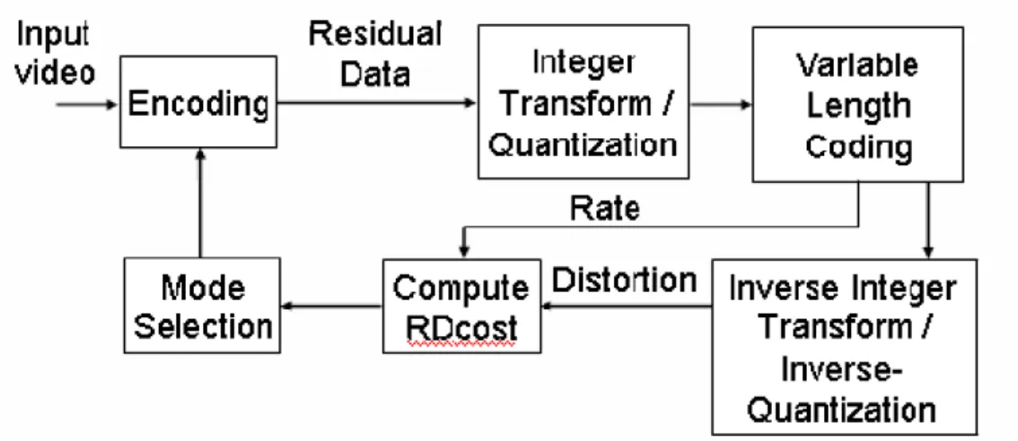
Figure 2.4：Computation of RDcost

To find the best prediction mode for better video coding performance, three variables should be take into consideration, there are quality, compressed bit rate and computational cost. The rate-distortion performance of video CODEC which describes the tradeoff between the first two components and the flowchart is shown in figure 2.4.

(2.1)

The function for RDcost computation is listed in Eq.2.1 (where Sk, Ik, Q,λMODE

represents the macro block number, mode number, quantize value and Lagrangian

parameter respectively). DREC is the estimation of distortion which measured by

calculating the sum of square value between the constructed and the original macro

block pixels. The RREC is the rate which produced after entropy coding. After

estimating all predictions for a macro block, the mode with minimum J is chosen as the suitable prediction. Totally, it performs 592 estimations to find the best prediction mode for a macro block and that must be the bottleneck of the real -time application as the resolution increasing.

)

,

(

)

,

(

)

,

,

(

S

I

Q

D

S

I

Q

R

S

I

Q

2.2.2 Researches of fast intra mode prediction

Fast intra mode prediction is a new topic in H.264/AVC and new methods are proposed every year. The main conception is reducing the times of calculation for RDcost by analyzing the processing block first. Some features extracted form the block or some algorithms among these modes may help to pick up the proper modes for the block. And then only those candidates are processed further to find the correct one.

It has developed many methods for fast intra prediction mode decision. Basically, it can be divided into three classifications about the processing methods of this topic. The first classification is using the charac teristics extracted form the block to avoid the unnecessary computation. The second classification is dividing the prediction modes into groups by the corrections extracted from them and only the modes of selected group are processed in next. The third is to modify the specifications of H.264/AVC, keeping a parallel and pipelined execution of intra prediction. Lots information for intra prediction is not used in the second type so the coding efficiency may drop. The parallel and pipelined type has high hardware spend and needs to modify the standards so we don’t take it into consideration either.

2.3 Edge based fast intra mode prediction mode decision

Edge based fast intra mode prediction is the method proposed by Pan which use the information of objective edge to find the suitable modes for a block. Comparison with other methods, this method only needs the spatial analysis so most of them can be easily implemented with lower hardware spends. The experimental results also show that the method improves the coding speed significantly with negligible loss of the quality. And that is the goal of our design for this issue.

2.3.1 Observation and scheme

The edge based fast intra mode prediction method is based on the observation. The pixels along the direction of loca l edge usually have the similar values. (Both luma and chroma components are the same) If the pixels are predicted by the neighboring pixels which are in the same direction of the edges, a good prediction can be found.

The method mainly include two procedures, the first one is in charge of generating values which can represent the features (including amplitude and direction) of a small part of a block. That information is stored or accumulated while the second procedure would pick up the proper modes for the processing block base on this information.

2.3.2 Related works

There are three related works of the edge based method about our research would be discussed in this paragraph. All of the tree works have the similar procedure, finding the proper results by managing the information of the virtual points generated in the beginning, but different algorithms and designs.

In the work of [2], in order to find the edge in formation in the adjacency of the intra block to be predicted, the edge map of the image is pr oduced by the Sobel edge operators. Each pixel is related with a part in the edge map, which is the edge vector including its edge direction and amplitude. The Sobel operator contains two convolution cores which are charge in calculating the difference in both vertical and horizontal directions. And the operator can be described as

(2.2) 1 , 1 1 , 1 , 1 1 , 1 1 , 1 , 1 ,j



i j



2



ij



i j



i j



2



ij



i j i

p

p

p

p

p

p

dx

1 , 1 , 1 1 , 1 1 , 1 , 1 1 , 1 ,j



i j



2



i j



i j



i j



2



i j



i j i

p

p

p

p

p

p

dy

(2.3)

(Where and represent the difference in vertical and horizontal directions respectively and is the value of pixel in i -th column and j-th row). If an edge vector is defined as , then the amplitude and direction of the edge vector can be estimated by the formulas below.

(2.4)

(2.5)

In order to decide the proper modes for prediction, an edge direction histogram is established from all the pixel map of the block by accumulating the amplitude of the edge with similar directions in the block. And the directions of the histogram are decided by the following rules, Eq.2.6 is for 4 x 4 block and Eq.2.7 is for 16 x 16 block. For 8 x 8 chroma blocks, it has equation similar to Eq.2.7 except that the order of mode numbers is different. (2.6) j i

dx

_,

dy

_i,j



ij ij



j i

dx

dy

D



_,



_,

,

_, j i j i j i dx dy D Amp(_, ) _,  _,     180 arctan( ), ( ) 90 ) ( _, , , , ij j i j i j i Ang D dx dy D Ang    j i

p

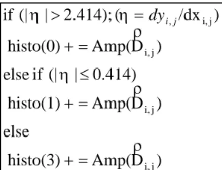
_, ) D Amp( histo(8) 0.199) -| | (-0.668 if else ) D Amp( histo(3) 0.668) -| | (-1.497 if else ) D Amp( histo(7) 1.497) -| | (-5.027 if else ) D Amp( histo(5) 5.027) | | (1.497 if else ) D Amp( histo(4) 1.497) | | (0.668 if else ) D Amp( histo(6) 0.668) | | (0.199 if else ) D Amp( histo(1) 0.199) | (| if else ) D Amp( histo(0) ) /dx ( 5.027)}; | (| or 0)] (dy and 0) {[(dx if j i, j i, j i, j i, j i, j i, j i, j i, , j i, j i,                                                   dyij

(2.7)

There are totally eight cells in 4 x 4 block histogram and three cells in macro block (16 x 16 block) histogram because the DC mode is always chos en in accordance with experiment. For the 4 x 4 block intra prediction mode decision, the cell which has the maximum amplitude and its two adjacent cells are chosen with DC mode to perform the further RDO calculation. For the macro block intra predication mode decision, only two modes are take care of the RDO calculation. Therefore, the total calculations of intra prediction mode decision can be reduced massively and the processing speed is raised also.

Another solution for this issue is proposed in [ 3] and its algorithm is introduced in figure 2.5. Any image-block (including 4 x 4, 16 x 16 and 8 x 8 block size) can be seen as a composition of four sub -blocks. And we can get a 2 x 2 pseudo-block with a0, a1, a2 and a3 pixel values which are produced by averaging all pixels of each sub-block.

Figure 2.5：Definition of pseudo-block

) D Amp( histo(3) else ) D Amp( histo(1) 0.414) | (| if else ) D Amp( histo(0) ) /dx ( 2.414); | (| if j i, j i, j i, j i, ,                dyij

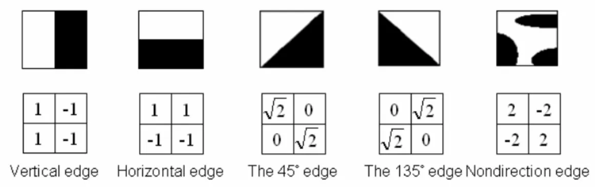
Figure 2.6：Five type of directional filter and its coefficients

There are five types of directional filter operated with the pseudo-block; they are vertical edge, horizontal edge, the 45° edge, the 135° edge and no-directional edge respectively and we show the illustrations and filter coefficients in figure 2.6. Each computational result represents the strength of the pseudo-block in that direction,

labeled Sv, Sh, S45°, S135°, Snd respectively. Eq.2.8 is the formula to find the strongest

direction of the pseudo-block and the modes which are related with this direction will

be performed further with the RDO computations. For example, if Sv is the maximum,

mode 0, mode 2, mode 5 and mode 7 are chosen for RDO calculation of the 4 x 4 block.

(2.8)



_Sv _Sh _{S S S}nd



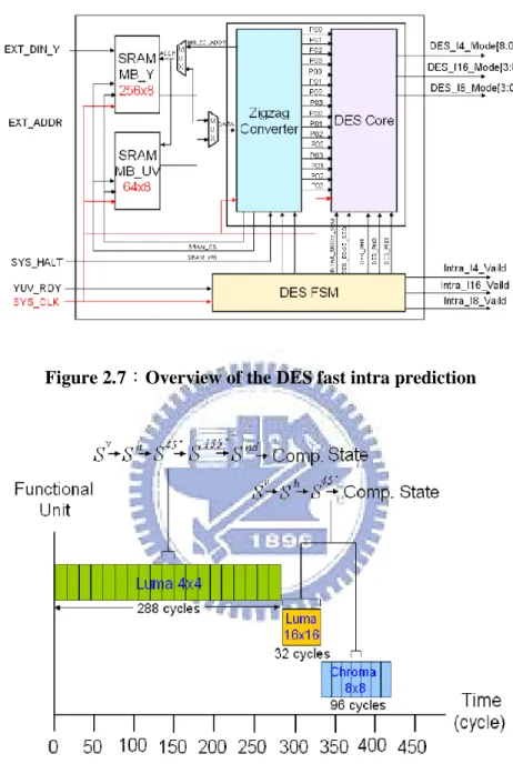
nd h v Ep , , , , , 135 , 45 , , max arg 45 135   

Figure 2.7：Overview of the DES fast intra prediction

Figure 2.8：Timing schedule of the DES engine

Figure 2.7 and 2.8 is the whole structure and timing schedule of this design respectively. The zigzag converter is connected with memory for arranging the image data which is in the raster scan order to the zigzag scan order. The DES core is main

design which responsible for pseudo -block computation, edge fi ltering and dominant edge strength extraction. The DES FSM is charge of generating the timing schedule of the architecture. The time spend for one macro block, including both luma and chroma components, is 416 cycles.

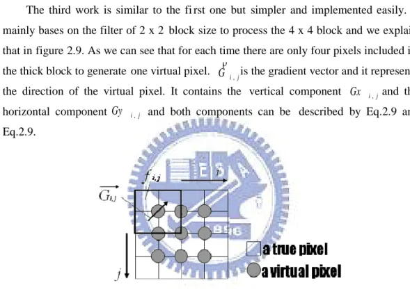
The third work is similar to the fi rst one but simpler and implemented easily. It mainly bases on the filter of 2 x 2 block size to process the 4 x 4 block and we explain that in figure 2.9. As we can see that for each time there are only four pixels included in

the thick block to generate one virtual pixel. is the gradient vector and it represents

the direction of the virtual pixel. It contains the vertical component and the horizontal component and both components can be described by Eq.2.9 and Eq.2.9.

Figure 2.9：A 2 x 2 filter for gradient vector calculation

(2.9)

(2.10)

The amplitude of the virtual pixel is the absolute sum of Gx and Gy and be explained by Eq.2.11. The other important information of the virtual pixel .i.e. the direction can be decided by the modified algorithm listed as Eq.2.12.

j i G , 

2

,

1

,

0

,

)

(

)

(

_{, 1 1, 1 , 1,} ,



f





f

 



f



f



i

j



Gx

_{i j i j i j i j i j}

2

,

1

,

0

,

)

(

)

(

_{1, 1, 1 , , 1} ,



f





f

 



f



f



i

j



Gy

_{i j i j i j i j i j} j i Gx _, j i Gy _,

(2.11)

(2.12)

The err is the difference of | Gx | and | Gy | in different weight. As we can see those weights are just different powers of two so they need only shift operator for implementation. The minimum err is the proper direction of this virtual pixel and should be keep in the edge direction histogram like the first work, so does the second-minimum err. Finally, the suitable modes for the processing 4 x 4 block are chosen by managing the histogram and calculated for RDO computations. It only needs four modes for 4 x 4 blocks, three modes for 16 x 16 and 8 x 8 blocks.

j i j i j i

Gx

Gy

G

Amp

(



_,

)





_,



_, j i j i Gx Gy err₀  _, 8 _, j i j i Gx Gy err₁ _, 0.125 _,         else Gx sign Gy sign Gx Gy err i,j 1 i,j ( ( i,j) ( i,j)) 3         else Gx sign Gy sign Gx Gy err i,j 1 i,j ( ( i,j) ( i,j)) 4         else Gx sign Gy sign Gx Gy err i,j 2 i,j ( ( i,j) ( i,j)) 5         else Gx sign Gy sign Gx Gy err i,j 0.5 i,j ( ( i,j) ( i,j)) 6         else Gx sign Gy sign Gx Gy err i,j 2 i,j ( ( i,j) ( i,j)) 7         else Gx sign Gy sign Gx Gy err i,j 0.5 i,j ( ( i,j) ( i,j)) 8

Figure 2.10：Block diagram of the VLSI architecture of fast IPMD

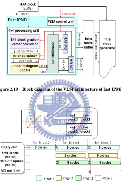
Figure 2.11：Timing schedule of the fast IPMD

Figure 2.10 is the whole VLSI structure of Li ’s design [4], and its timing schedule is shown in figure 2.11. This structure can be divided into two parts. The first part,

including 4 x 4 block gradient vec tor calculator, error calculator and linear histogram update, is responsible for computing the mode information of each virtual pixel. The rest part manages the histogram which stores the information of each virtual pixel of 4 x 4 blocks to find the proper modes for the 4 x 4 block. In respect of the processing time, because of the reusing information of 4 x 4 blocks, it doesn’t spend another time for macro block processing. And the total time spend for one macro block is 170 cycles.

2.3.3 Summary

Table 2.2：Comparison of the related works Related work 1 (Peng’s) Related work 2 (Wang’s) Related work 3 (Li’s) Algorithm

complexity High Middle Low

Hardware

spend NA 10.3k 15.8k

Table 2.2 is a short summary of the three related works we talk about above. From table 2.1, we hope to propose architecture not only to speed up the intra prediction mode decision in H.264/AVC but also with low complexity in our research. The Peng’s work has highest complexity and we won ’t take it into consideration. The Li’s work can be implemented simpler but higher hardware spends than Wang’s. However, there is still some improvement can do with Li’s design.

In Wang’s research, the zigzag converter is in charge of re -ranging the data order and therefore the complexity of the DES core is reduced, hardware spend is decreased also. Here we use this conception in our design to modify the Li ’s research and achieve our goal.

Chapter 3

The proposed modified architecture

In the beginning of this chapter we give the conspectus of the whole pr oposed structure in detail, including the algorithm, data size, timing schedule of our design. And then we will explain each part particularly of our proposed architecture.

3.1

Overview of the proposed architecture

The whole modified structure we design for edge based fast intra mode decision is

showed in figure 3.1.The main architecture is composed of five components; including

4 x 4 block gradient vector cal culator, direction decision, histogram unit, 4 x 4 block mode decision and micro block mode decision. The 4 x 4 block pixels are stored in the 4 x 4 block buffer and those data can be used by the intra mode generator also. The intra mode buffer stores the candidate modes generated by the fast intra prediction mode decision, each prediction mode is represented with one bit ( ‘0’ for “disable” and ‘1’ for

“enable”, respectively). The finite state machine (FSM) control unit is responsible for

holding the timing schedule of the system.

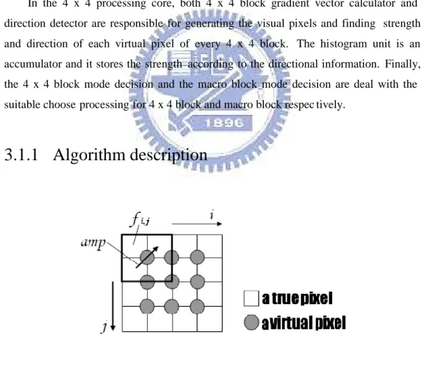
In the 4 x 4 processing core, both 4 x 4 block gradient vector calculator and direction detector are responsible for generating the visual pixels and finding strength and direction of each virtual pixel of every 4 x 4 block. The histogram unit is an accumulator and it stores the strength according to the directional information. Finally, the 4 x 4 block mode decision and the macro block mode decision are deal with the suitable choose processing for 4 x 4 block and macro block respec tively.

3.1.1 Algorithm description

In the beginning of the schedule, four pixels are fetched to a 2 x 2 filter (the thick block in figure 3.2) to calculate the value of virt ual pixel. There are total nine virtual pixels for each 4 x 4 block to decide the proper mode and each virtual pixel include the vertical value Gx and horizontal value Gy. Both of them are calculated by the formulas below：

(3.1)

(3.2)

Based on the values of Gx and Gy, the strength (amp) of the virtual pixel is the sum of the absolute value of Gx and Gy (Eq.3.3) and the direction can be decided by the sign information of Gx and Gy and Eq.3.4, 3.5, 3.6.

(3.3) (3.4)

(3.5)

(3.6)

As shown in figure 3.3, th e sign information of Gx and Gy divide the plane to four parts. If the sign of Gx is the same as Gy, the direction would cross the quadrant of first and third. Otherwise, it cross the quadrant of second and fourth; and further, Eq.3.3, 3.4, 3.5 can be the judgment to find the final answer for the current 4 x 4 block.

)

(

)

(

_{, 1 1, 1 , 1,} ,j i j i j i j i j i

f

f

f

f

Gx



_



_{ }





_

)

(

)

(

_{1, 1, 1 , , 1} ,j



i j



i j



i j



i j i

f

f

f

f

Gy

|

|

2 Gy

Gx



|

| Gy

Gx



|

|

2 Gx

Gy



j i j i

Gy

Gx

amp





_,



_,

Figure 3.3：The modified intra prediction mode direction (4 x 4 block)

The strength above then is stored separately according to the directional information. There are only eight modes be taken into consideration because the DC mode always be chosen for the rate -distortion cost (RDcost) calculation and therefore we can neglect it.

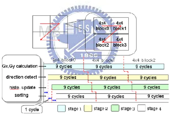
In the final part of our design, we always choose the top three modes which are strong in direction together with mode 2 for the RDcost calculation for each 4 x 4 block. As we can see there always be two adjacent modes be decided for one virtual pixel of a 4 x 4 block in every cycle. For the reason of reducing size, we can ’t sort the directional values to find the proper modes until all virtual pixels are processed completely because that would need huge hardware to do the eight values sorting and spend another time for this process. Therefore, we do the sorting processing ev ery cycle with only five data should be take care, including two new generating mode values and three mode values produced in former cycle. And the suitable modes for each 4 x 4 block will be given in the period of nine cycles. For macro block, it needs 14 4 cycles to get the proper modes.

3.1.2 Timing schedule of the proposed hardware

The timing schedule of our design is shown in figure 3.4; the scan order of the 4 x 4 block is still zig-zag manner as the specification of H.264/AVC and processed sequentially. The first stage is responsible for generating the virtual pixel and each virtual pixel will be sent to next stage one by one as the cycle going. Averagely it needs only nine cycles to process one 4 x 4 block.

3.2

The modified memory access scheme

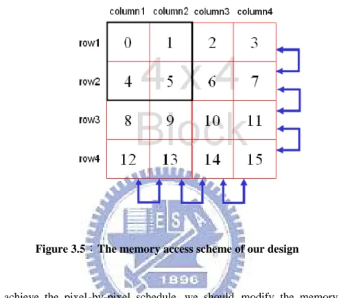
Figure 3.5：The memory access scheme of our design

To achieve the pixel-by-pixel schedule, we should modify the memory access scheme in the beginning and figure 3.5 is the access method used in our design. In the earlier three cycles, row 1 and row 2 are fetched and held; only the pixels which belonged to column 1 and column 2 are used for generating the virtual pixel (i.e. pixels inside the black block in figure 3.5). In next cycle, we move the black block one step right and choose the pixels included in it also (i.e. pixel 1, 3, 4 and 6) to generate the second virtual pixel. This procedure totally needs nine cycles to produce all virtu al for one 4 x 4 block.

3.3

The modified 4x4 gradient vector calculator

same value inside the parenthesis but different sign in the first part. So it only needs four computations to get Gx and Gy, and we can implement that easily with butterfly architecture.

(3.7)

(3.8)

Figure 3.6：Architecture of the gradient vector calculator

Figure 3.6 illustrates our design of the gradient vector calculator; it is composed of four adders and separated into two levels. The top two adders compute the value inside parenthesis of Eq.3.7, 3.8. The ot her two adders below compute the values of Gx and

Gy first and then the operation of absolution would be done according to the sign bits of Gx and Gy. The absolution values and sign information will be used in the next stage.

In the digital video, each pixel value is represented in a range from 0 to 255. But the top two adders of our design are operated in subtraction and the range of Gx and Gy

)

(

)

(

_{1, , 1 1, 1 ,} ,j i j i j i j i j i

f

f

f

f

Gx





_



_



_{ }



)

(

)

(

_{1, , 1 1, 1 ,} ,j i j i j i j i j i

f

f

f

f

Gy





_



_



_{ }



would be -510 to +510. Hence each data in this hardware is represented in 10 -bits, including the output. It is be cause that although the output are absolute value and its ’ range is form 0 to 510, but we will double the values for comparison in the next stage and that needs 10-bits data size for representation.

3.4

The modified direction detector

According to the discussi on in paragraph 3.1.1, we can implement the modified intra prediction mode decision without any multiplications and this advance not only keeps our hardware small but also raises the operating speed. Here we give a name called direction detector in our design to avoid confusing with others’ design.

Figure 3.7：Direction detector

Figure 3.7 is the architecture of direction detector in whole; the adders in color are the part of gradient vector calculator which we discussed before. Here we need the sign bit of the Gx and Gy to decide the possible quadrants which would be crossed by the

direction of virtual pixel. All hardware we need to do this job is just a XNOR gate and the output of the XNOR gate is the first bit of range informa tion. We list the relation between the sign of Gx and Gy, logic output of XNOR and the direction of virtual pixel in table 3.1.

Table 3.1：Relation between sign bits, XNOR and direction of virtual pixel

Sign_Gx Sign_Gy XNOR Direction of virtual pixel

0

0

1

1, 3 quadrant

0

1

0

2, 4 quadrant

1

0

0

2, 4 quadrant

1

1

1

1, 3 quadrant

The second bit and third bit of range information are prod uced by the three comparators in figure 3.6. The top one executes the judgment in Eq.3.4 and the other two comparators below process the operation of Eq.3.5 and Eq.3.6 respectively. The output of top comparator is sent to next stage as the second bit of ra nge information and to a multiplexer too. According to this bit, the multiplexer chooses the third bit of range information from the outcome of the two comparators below.

The range information bits are composed of three bits and used to select the proper modes for current virtual pixel. Each data pick up two adjacent modes and there are totally eight combinations for 4 x 4 block and two combinations for macro block. Table 3.2 lists all situations of range information bits and the relative modes.

Table 3.2：Mode select scheme Direction information bits Selected mode (4 x 4 block) Selected mode (macro block)

000

0, 7

0, 3

001

7, 3

0, 3

010

3, 8

1, 3

011

8, 1

1, 3

111

1, 6

1, 3

110

6, 4

1, 3

101

4, 5

0, 3

100

5, 0

0, 3

There is still an adder to comp ute the sum of the absolute values of Gx and Gy and it is the strength of the processing virtual pixel. The data size of the outcome in this adder is 9-bits and it is because Gx and Gy can’t be maximums at the same time; as we can see in Eq.3.7 and Eq.3.8, when Gx is maximum, Gy become zero, and vice verse, that means the maximum of the absolute value won’t be over 510 and the sign bit of the absolute value is always zero so we can neglect the sign bit and sent the other bits to the next stage. Both the range information bits and the strength of virtual pixel are sent to the next hardware for accumulations.

3.5

The histogram accumulator

Figure 3.8：Architecture of the proposed histogram unit

The histogram unit is responsible for accumulations and its’ whole structure is shown in figure 3.8. The right part is used for 4 x 4 block process while the left part is used for macro block process. There are 11 registers (labeled r1, r2 … and r11 respectively) used in this hardware, each of them represent a mode of the defaults used in H.264/AVC intra prediction beside the DC mode (mode 2 in 4 x 4 block and macro block). The data size of a register is 13 -bits and 17-bits for 4 x 4 block and macro block respectively. Here we take the 4 x 4 block process for example and describe it below.

In the beginning, based on the range information which is given by the former unit, the multiplexers pick up two registers form r1 to r8, both selected registers are adjacent modes (or directions) in figure 3.3 . Then the amplitude (amp) of the current virtual pixel will be added to these two registers. Besides using in the next stage, the outputs of the adders are sent back to update the old values of selected registers also and we can use

Eq.3.9 to describe that (where i is the cycle number and r is the selected register). A ll the values of registers are cleared to zero in the periods of nine because there are nine virtual pixels in a 4 x 4 block only.

(3.9)

The macro block is processed in the similar way but the values of registers are set to zero when all virtual pixels in a macro block are processed and it needs 144 cycles for a period.

The mode information generator the mode information based on the range information bits that we have listed in table 3.2. And this mode information will be used by the 4 x 4 block mode decision and macro block mode decision in the next stage.

3.6

The proposed sorting hardware for 4x4 and macro

block

Figure 3.9 is the whole structure of the 4 x 4 block mode decision which is divid ed into three parts; they are zero setting comparator, sorter and top three selector. R1, R2 and R3 are registers of the zero setting comparator ; I1 and I2 are input mode information which comes from the former unit. Each of them contains two parts; mode and amplitude, and we use R1m, R2m … to represent the mode part and R1a, R2a … to represent the amplitude part in the discussion below. R1’, R2’ and R3’ are the arranged output and they have amplitudes in the order of R1m ’ > R2m’ > R3m’. These information of R1’, R2’ and R3’ are sent back to replace R1, R2 and R3 respectively in the next cycle. The selecting algorithms of the 4 x 4 mode decision will be discussed below.

)

8

...

2

,

1

(

1









r

amp

i

r

_{i i i}

Figure 3.9：Structure of the 4 x 4 block mode decision

The whole structure is in charge of choosing the top three proper modes of a 4 x 4 block. In each cycle of the procedure, two input I1 and I2 are fed to this structure, including the mode information I1m, I2m and the amplitude information I1a, I2a. The modes of input are checked in the first stage to confirm that whether the input modes are equal to the modes of registers or not. If it is true, that means the amplitude of this mode has been accumulated again in th e former unit. And then the associated amplitude of register is set to zero. This step can promise the new selected modes of the output won’t be the same as another during each cycle..

Stage two and stage three both together arrange the amplitude in the decreasing order. And the top three amplitudes and the associated modes are chosen as the output. Because the amplitude of the register which has the same mode as the input have been set to zero. It is hard to be the selected one, so the problem of equal mod e selecting can be avoided. After all virtual pixels of a 4 x 4 block are processed, the outcome is acquired also.

Figure 3.10：Zero setting comparator

The architecture of the zero setting comparator is shown in figure 3.10 and we can see there are three uniform modules compose the hardware. Each of them performs a check between register R and input I and only the mode information are used here. If the output of the OR gate is 1, then multiplexer will choose zero as the output. The six outputs of equality comparators in figure 3.10 are used in next stage also so they are sent with the three amplitudes of multiplexers to the second stage.

Figure 3.11 is our design for sorting procedure, and it needs three multiplexers and the selection generator. There are three 16-bits input of each multiplexer and each 16-bits input is divided two parts. The first 3-bits are the mode information and the rest 13-bits represent the amplitude information and connected with the output of the former. The selection generator is in charge of re -ranging the output in the decreasing order (i.e. O1 > O2 > O3) based on the 6 -bits input which is a collection of the output of six equality comparators in former stage. And the selecting algorithm is given in table 3.3.

Table 3.3：Sorting algorithm of the sorter (4 x 4 block)

Output

Comparator 1,3,5 Comparator 2,4,6

_O1

_O2

_O3

000 000 R1 R2 R3 000 100 R2 R3 R1 000 010 R1 R3 R2 000 001 R1 R2 R3 100 000 R2 R3 R1 100 010 R3 R1 R2 100 001 R2 R1 R2 010 000 R1 R3 R2 010 100 R3 R1 R2 010 001 R1 R2 R3 001 000 R1 R2 R3 001 100 R2 R1 R3 001 010 R3 R1 R2

Figure 3.12：Architecture of the top 3 selector

The top three selector is third stage of the 4 x 4 mode decision and we can see it in figure 3.12. Its architecture is similar to the sorter but more complex. There are seven comparators used to compare all amplitudes and the outputs are sent to the selection generator. And we list the selecting algorithm in table 3.4.

Table 3.4： Selecting algorithm of the top 3 selector

Output

Comparator 1 Comparator 2~4 Comparator 5~7 _{R1’ R2’ R3’} 1 111 111 I1 I2 R1’ 0 111 111 I2 I1 R1’ Don’t care 111 011 I1 R1’ I2 Don’t care 111 001 I1 R1’ R2’

Don’t care 111 000 I1 R1’ R2’ Don’t care 011 111 I2 R1’ I1 1 011 011 R1’ I1 I2 0 011 011 R1’ I2 I1 Don’t care 011 001 R1’ I1 R2’ Don’t care 011 000 R1’ I1 R2’ Don’t care 001 111 I2 R1’ R2’ Don’t care 001 011 R1’ I2 R2’ 1 001 001 R1’ R2’ I1 0 001 001 R1’ R2’ I2 Don’t care 001 000 R1’ R2’ I1 Don’t care 000 111 I2 R1’ R2’ Don’t care 000 011 R1’ I2 R2’ Don’t care 000 001 R1’ R2’ I2 1 000 000 R1’ R2’ R3’ 0 000 000 R1’ R2’ R3’

The whole structures of the macro block mode decision are shown in figure 3.13. As we can see that it is designed different from the architecture of the 4 x 4 block mode decision. Only two modes are chosen as output b ecause we just need two proper modes only for a macro block to run the rate -distortion computations.

For a macro block, there are 16 4 x 4 block and each of them take 9 cycles for processing. So the macro block mode decision module need to be operated in every 144 cycles, and all amplitudes are accumulated in the further module first before operating. Here we listed the selecting algorithm of the macro block mode decision in table3.5.

Table 3.5：Selecting algorithm of macro block mode decision

Output

Comparator_1 Comparator_2 Comparator_3

O1

O2

1 1 1 Mode_0 Mode_1 1 0 1 Mode_0 Mode_3 0 1 1 Mode_1 Mode_0 0 1 0 Mode_1 Mode_3 1 0 0 Mode_3 Mode_0 0 0 0 Mode_3 Mode_1

Chapter 4

Implementation results

Chapter 4 is the simulation results of our design and it is composed of three paragraphs. The simulation environment is introduced shortly in the first paragraph. And the results are presented in detail in the next paragraph. Here some advantages of our hardware would be accentuated by comparing with other architectures. At last, some improvements which can make our hardware more efficient ar e discussed for future work.

4.1

The simulation environment

The module we proposed is written in programs of the language of Verilog1995 and simulated in Modelsim 6.1 environments. For the procedure of synthesis, all programs are compiled with Verilog -XL in Synposys system. Our design is implemented with TSCM 0.18 μm technology for estimations of gate counts, power dissipation and maximum operating frequency.

4.2

Comparison with other architectures

The architecture we proposed is a modified design for [4], and the outcome of our design is the same as [4] (i.e. our module can choose the same modes as [4 ] for a block). Therefore, the proposed architecture can also k eep the same image quality as [4 ]. The main comparisons of our research are the hardware design and spend; here we will talk

about the main modified parts in de tail.

The algorithm of the object which we modified reduces the total RDO computations from 592 to 198 or 132, with about 66% decrease and a negligible quality loss. Figure 4.1 and figure 4.2 are the RD curves of the video sequence ‘stefan’ and

‘parkrun’ (Qp = 24, 28, 32, 36) which have the fast moving and highly detailed contexts.

Other video test results are listed in table 4.1.

Figure 4.1：RD-curve stefan (CIF, 150 frames)

Table 4.1：Performance of the architecture on various video sequences Sequences △Bitrate (%) △PSNR (%) Bus* 1.80 -0.08 Coastguard* 1.57 -0.06 Container* 0.57 -0.02 Football* 5.57 -0.28 Husky* 1.00 -0.08 Mobile* 2.29 -0.11 Panzoom* 1.97 -0.06 Paris* 2.52 -0.11 Silent* 2.86 -0.10 Stockholm* 2.21 -0.09 Table* 2.28 -0.09 Tempete* 2.29 -0.10 City** 0.54 -0.01 Crew** 2.23 -0.05 Harbour** 1.98 -0.07 Knightshields** 1.37 -0.03 parkrun** 0.97 -0.05 *：CIF**：1280x720p

Table 4.1 is the simulation results extracted from [5] of varies video stream. As we can see from table 4.1, a maximum bit rate overhead is found (5.57%) as well as a maximum PSNR drop (0.28db) for the sequence ‘football’. In the other cases, only small bit rate overhead (less than 3%) and almost negligible PSNR loss (less than 0.2db) is assumed.

hardware spend and higher processing efficiency, and the detail of original design and the modified scheme are discussed below.

Figure 4.3：Architecture of the gradient vector calculator

Figure 4.4：Pixel access rule

The original architecture of the gradient vector calculator is shown in figure 4.3 and its access scheme is illustrated in figure 4.4. It needs nine cycles to calculate all the

gradient vectors of a 4 x 4 block. In each cycle, four pixels are loaded from the 4 x 4 block buffer with three subtractions are processed simultaneously. In the earlier four cycles, pixels are fetched in row by row and the Gx components are calculated. In the later four cycles, the other components Gy are processed. And we can realize that it needs a register array to store the partial resul ts.

In our design, the conception similar to the second related work we talk about in chapter two is used i.e. arranging the input data in the efficiency way for processing. And in each cycle, one virtual pixel ( Gx and Gy) is produced, therefore the regist er array can be removed and the adders are abated also.

Figure 4.5：Histogram cell update control

According to the components of Gx and Gy, the original design uses the algorithm we listed in Eq.2.12. The implementation of the algorithm needs at least eight adders processing simultaneously and an extra hardware to deal wi th the sign bits. The generated values (i.e. err0, err1, err3 …and err8) are processed by the histogram cell update control which is shown in figure 4.5. Since the mode with second -minimum error must be the adjacency of the minimum one, the minimum finding hence are first done between err0, err1, err3 and err4, relating to mode 0, mode1, mode3 and mode4. And the results are used to find the second -minimum error.

The architecture we proposed uses the sign bits as the judgment of directions, and the components of Gx and Gy (which have the same data size as err) are processed directly also. Therefore, we just need three comparators to perform this procedure. And the adders and the histogram cell update control can be replaced. Table 4.2 is the comparisons of hardware spend among our design and Li ’s in the main module of the 4 x 4 block processing core. As we can see that the hardware cost is very low in our proposal.

Table 4.2：Comparison of hardware spend in the main module

Li’s

Proposed design

Vector calculation Error calculation Vector calculation Direction decision #Adder 6 8 4 1 #Comparator 0 7 0 3 #Register 18 0 0 0

There still another modified in our design of the mode decision parts and we take the 4 x 4 block mode decision for example only. In the 4 x 4 block processing core, the histogram unit is in charge of holding the amplitudes of each mode. If we perform the procedure of mode decision after all amplitudes of the virtual pixels processed. It needs to re-range an eight -cells row in the decreasing order with 28 comparisons, which is too expensive for implementation.

In our proposal, the procedure of mode decision is executed when a virtual pixel produced. And it is only five components which need to be re-ranged and the comparisons can be reduced to 10. But we design this module in three stages; the information generated in the first stage is used in the second stage i.e. the sorter. Hence three comparing operations can be decreased. Finally, the hardware spend for the 4 x 4