無線感測網路中繼節點佈建方法之研發-以室內環境為例

(1)

國

立

交

通

大

學

電機學院 IC 設計產業研發碩士班

碩

士

論

文

無線感測網路中繼節點佈建方法之研發-以室內環境為例

Development of a Relay Node Deployment Method for Disconnected Wireless

Sensor Networks: Applied in Indoor Environments

研究生：劉蓓縝

指導教授：唐震寰教授

(2)

無線感測網路中繼節點佈建方法之研發-以室內環境為例

Development of a Relay Node Deployment Method for Disconnected Wireless

Sensor Networks: Applied in Indoor Environments

研究生：劉蓓縝 Student：Pei-Chen Liu 指導教授：唐震寰 Advisor：Jenn-Hwan Tarng 國立交通大學電機學院 IC 設計產業研發碩士班碩士論文 A Thesis

Submitted to College of Electrical and Computer Engineering National Chiao-Tung University

in partial Fulfillment of the Requirements for the Degree of

Master

in

Industrial Technology R & D Master Program on IC Design

July 2007

Hsinchu, Taiwan, Republic of China

(3)

無線感測網路中繼節點佈建方法之研發-以室內環境為例

學生：劉蓓縝指導教授：唐震寰國立交通大學電機學院IC 設計產業研發碩士班

摘要

中繼節點佈建方法乃是用較少量的中繼節點佈建於適當的位置以增進無線感測網路的通訊品質。由於無線感測網路的感測節點廣泛的應用在各個領域，為了讓節點間達成無線通訊的行為，必須在不相連的節點中有效的佈建中繼節點，因此如何有效地佈置中繼節點是個困難且耗費時間的問題。本論文係以二維幾何搜尋演算法為基礎並採用無線電傳播效應之網路拓撲評估模式，提出一種嶄新的無線感測網路中繼節點佈建方法，其特性分別為逐一計算每個候選中繼節點連接至其所有鄰近節點的數量，並根據鄰近節點的連接數，選擇一個擁有最多鄰近節點的候選中繼節點而佈建；以及藉由精確評估鏈結狀態方法來決定網路拓撲型態。模擬的結果指出本研究所提出之佈置中繼節點方法與相關文獻所提之佈建方法相比，本方法大幅降低中繼節點的佈建數量，其中在網路節點密度為 1/250 節點數/平方公尺的條件下，本文所提出之精確評估鏈結狀態方法對中繼節點的佈建數量的改善，降低 30% 的中繼節點之佈建數量；而二維幾何搜尋演算法亦可降低 20% 的中繼節點之佈建數量。關鍵詞：無線感測網路、佈建、中繼節點

(4)

Development of a Relay Node Deployment Method for Disconnected Wireless Sensor Networks: Applied in Indoor Environments

Student：Pei-Chen Liu Advisor：Jenn-Hwan Tarng

Industrial Technology R & D Master Program on IC Design of Electrical and Computer Engineering College

National Chiao Tung University

ABSTRACT

The connectivity of a given static, disconnected wireless sensor network can be improved by deploying additional relay nodes in the network, forming connections between separate clusters of connected nodes. Finding optimal locations to place the relay nodes is a difficult and time-consuming problem. In this research, we propose a heuristic relay node deployment method to provide more efficient relay node deployment comparing to related works. In this method, a two dimension geometric search algorithm is proposed to discover a proper location where adding a single relay node results in connecting as many as possible disconnected node pairs. Besides, in order to devise a practical method, a realistic model for link connectivity estimation and network topology determination is proposed, which takes into account radio propagation effects, including the large-scale path loss, shadow fading, and small-scale fading. Simulation results indicate that the proposed method significantly reduces the number of relay nodes required for repairing disconnected WSNs. There are about 20% of improvements contributed by the proposed two dimension geometric search algorithm, and about 30% of improvements donated by the proposed link connectivity estimation model.

(5)

誌謝

本論文得以順利完成，首先要感謝我的指導教授唐震寰博士的悉心指導，於研究期間不時的意見交流與耐心解惑並指點我正確的方向。其次，尚需感謝在口試期間本校王蒞君博士與方凱田博士不吝提供建議與指正，使本論文更臻完備。另外，亦得感謝本實驗室莊秉文博士大力協助，感謝學長在專業的無線網路通訊領域中，不遺餘力的指導及鼓勵；以及特別感謝資管所學弟朝尉，在研究過程中的場景量測和MATLAB 程式上協助；此外要感謝的是，實驗室中美麗大方的梁麗君小姐，在兩年的研究生活中給予完善的協助。感謝 Allen、建傑、宜興、懷文學長們不厭其煩的指點我研究中的疏失，且在我迷惘時為我解惑，也感謝麻吉好友思云、實驗室同學亦慶、豐吉、育正、志瑋的幫忙，恭喜我們順利度過這兩年。當然也不能忘記實驗室的雅仲、俊彥學弟們的幫忙及搞笑，為實驗室添加了許多歡樂氣息。此外，男朋友文聖在背後的默默支持更是我前進的動力，謝謝他的體諒、包容，讓我這兩年的生活有很不一樣的光景。最後深深的感謝我親愛的家人，感謝你們在生活上與精神上的鼓勵和關懷，因為你們無悔的付出，我才得以完成學業。最後僅以此篇論文獻給我摯愛的家人、朋友以及所有關心我的人。劉蓓縝民國 96 年 7 月新竹

(6)

List of Tables

Table 3-1. The obtained value of the parameters from field test at 9th floor of Engineering Building 4, National Chiao Tung University...19

(8)

List of Figures

Figure 1-1. The general system blocks of a sensor node...1

Figure 2-1. MST-based relay node deployment method. ...7

Figure 2-2. An example of the MST-based relay node deployment method. ...8

Figure 2-3. MST-based relay node deployment method is not optimal. ...8

Figure 2-4. VW relay node deployment method. ... 11

Figure 2-5. An example of the VW relay node deployment method...12

Figure 2-6. VW relay node deployment method is not optimal. ...12

Figure 3-1. Flowchart of the proposed relay node deployment method...16

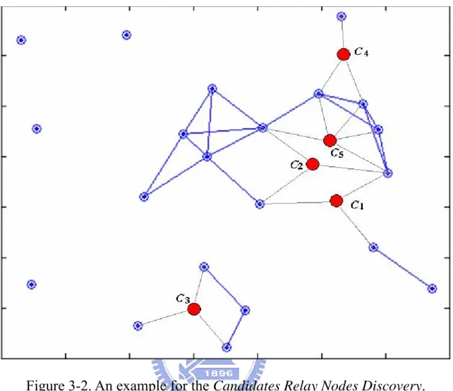
Figure 3-2. An example for the Candidates Relay Nodes Discovery. ...22

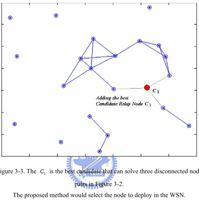
Figure 3-3. The is the best candidate that can solve three disconnected node pairs in Figure 3-2. ...24

1 C Figure 3-4. An example of proposed relay node deployment method...24

Figure 4-1. ANRN versus node density in LOS environment...29

Figure 4-2. Improvement ratio of ANRN versus node density in LOS environment...29

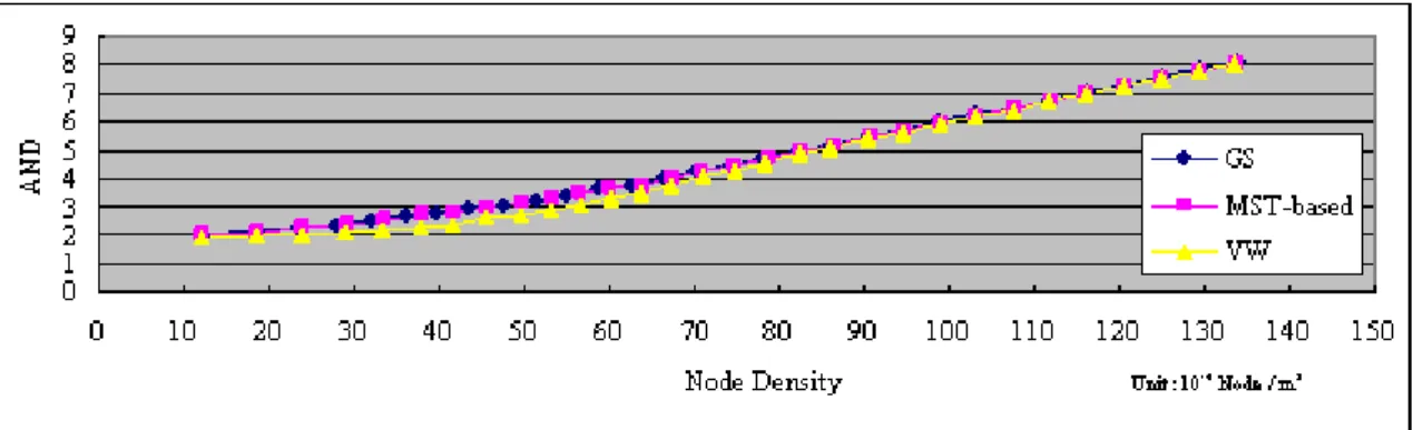
Figure 4-3. AND versus node density in LOS environment...30

Figure 4-4. ANRN versus node density in NLOS environment. (The partition loss of an obstacle is 7dB). ...31

Figure 4-5. Improvement ratio of ANRN versus node density in NLOS environment. (The partition loss of an obstacle is 7dB)...32

Figure 4-6. AND versus number of nodes in NLOS environment. (The partition loss of an obstacle is 7dB). ...33

Figure 4-7. ANRN versus node density in NLOS environment. (The partition loss of an obstacle is 15dB). ...34

Figure 4-8. Improvement ratio of ANRN versus node density in NLOS environment. (The partition loss of an obstacle is 15dB)...34

Figure 4-9. AND versus number of nodes in NLOS environment. (The partition loss of an obstacle is 15dB). ...35

Figure 4-10. ANNC versus node density in NLOS environment...36

Figure 4-11. ANRN versus node density in NLOS environment with small-scale fading....38

Figure 4-12. Improvement ratio of ANRN versus node density in NLOS environment with small-scale fading...39

Figure 4-13. AND versus number of nodes in NLOS environment with small-scale fading.40 Figure 4-14. ANNC versus node density in NLOS environment with small-scale fading....41

(9)

Figure 4-16. Improvement radio of ANRN versus number of initial nodes in LOS

environment...42

Figure 4-17. AND versus number of initial nodes in LOS environment...43

Figure 4-18. ANRN versus number of initial nodes in NLOS environment. ...45

Figure 4-19. Improvement ratio of ANRN versus number of initial nodes in NLOS environment...46

Figure 4-20. AND versus number of initial nodes in NLOS environment...48

Figure 4-21. ANNC versus number of initial nodes in NLOS environment. ...49

Figure 4-22. ANRN versus number of initial nodes in NLOS environment. ...51

Figure 4-23. Improvement ratio of ANRN versus number of initial nodes in NLOS environment...52

Figure 4-24. AND versus number of initial nodes in NLOS environment...53

(10)

1. Introduction

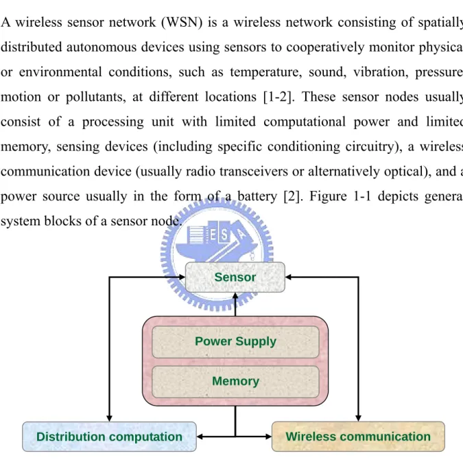
A wireless sensor network (WSN) is a wireless network consisting of spatially distributed autonomous devices using sensors to cooperatively monitor physical or environmental conditions, such as temperature, sound, vibration, pressure, motion or pollutants, at different locations [1-2]. These sensor nodes usually consist of a processing unit with limited computational power and limited memory, sensing devices (including specific conditioning circuitry), a wireless communication device (usually radio transceivers or alternatively optical), and a power source usually in the form of a battery [2]. Figure 1-1 depicts general system blocks of a sensor node.

Sensor

Power Supply

Figure 1-1. The general system blocks of a sensor node.

WSNs aim to achieve high reliability, flexible utilization, cost-effectiveness and ease of deployment. The problem of deployment of a WSN could be formulated generically as follows [3-4]: given a particular application context, and operational region, and a set of wireless sensor nodes, how and where

Distribution computation

Memory

(11)

should these nodes be placed? The cost and deployment constraints on sensor nodes result in corresponding wireless communication constraints on resources such as energy, memory, computational speed and bandwidth. Although it is very important to optimize the placement of sensors, it is often difficult to do that [5]. Two major performance metrics when deploying a WSN are considered in the literature: (i) Network Coverage, which measures the degree of covered sensing area of a given network, and (ii) Network Connectivity, which determines whether the network topology over which information routing can take place [6-10]. By considering network coverage, a rich number of works could be found in literatures. In [11], the authors provide a way to compute the minimum number of sensors needed for guaranteed coverage, and then deploy that number of sensors randomly in the target area. Some works focus on

κ-coverage [12-15], or even differentiated coverage deployment [16] whereby

higher degrees of coverage result in better localization accuracy and there is more tolerance of false activation of sensors.

By considering network connectivity, most research effects have been concentrated on either analyzing the asymptotic connectivity of large-scale WSNs [7, 9, 17] or devising topology control protocols to maintain connectivity in the presence of limited mobility [18]. In [7], Gupta and Kumar show that the

critical common range for connectivity of n randomly distributed wireless

nodes in a disk of unit area satisfies that, if

n r

( )

(

n c n

)

n r_n2 = log + π , the network is

asymptotically connected almost surely if

( )

=∞

∞

→ c n

nlim and is disconnected

asymptotically almost surely if

( )

=−∞

∞

→ c n

nlim . This result also implied by the

work of Penrose [17] on the longest edge of the minimal spanning tree of a

random graph. That , the length of the longest edge in the minimum

spanning tree of n points uniformly distributed in a unit square area, satisfies that n M

(

_π _α

)

− −α ∞ → − ≤ = e n nlimPr n M lnn e

(12)

node degree studied [9] from another angle by Xue and Kumar. They assumed the same number of nearest neighbors are maintained for each node, and showed that (i) the network is asymptotically disconnected with probability 1 as

increases, if each node is connected to less than nearest neighbors;

and (ii) the network is asymptotically connected with probability 1 as

increases, if each node is connected to more than nearest neighbors.

Further studied [10] the critical number of neighbors for

n n log 074 . 0 n n log 1774 . 5 κ-connectivity and

found the upper bound to be αe logn , where α>1 is a real number and

is the natural base.

718 . 2 ≈

e

WSNs are by nature constructed automatically, by the nodes connecting to the neighboring nodes and building up a network. In this context, the network topology is random, and in particular, no connectivity is guaranteed: the nodes may be so sparsely located that they are unable to make up a connected network. Besides, given that the connectivity of a WSN is susceptible to node mobility, node failure, and unpredictable environment influences, it is important to continuously maintain connectivity under all these unfavorable conditions. This has motivated the research with primary interest in the connectivity improvement by deploying relay nodes for a given disconnected network.

To the best of our knowledge, little attention has been paid to improving network connectivity or repairing disconnected network by deploying additional nodes. Besides, most of existing works utilize a deterministic physical model, the Unit Disk Graph model [6], for representing network connectivity, which ignores signal attenuation and fading effects of wireless communications. In order to properly estimate network connectivity, more realistic models such as probabilistic graph model [6, 19] are need.

(13)

2. Problem Definition and Related Works

2.1 Problem Definition

We consider the problem of deploying additional relay nodes to improve the connectivity of an existing WSN. Specifically, given a disconnected WSN, we investigate how to deploy as few as possible additional relay nodes to connect all existing nodes. Here we define the investigating problem as Relay Node

Deployment problem in WSNs. Let the initial network topology be represented

by an undirected simple geometric graph G =

(

V,E

)

in a Euclidean plane R2,

where V =

{

v₁,v₂,_K,v_n

}

is the set of initial sensor nodes. E is the set of links

and is defined by E =

{

( ) ( )

a,b :l a,b >λ,a,b∈V

}

, where denotes the

estimated probability that a message is correctly transmitted from node to node , and

( )

a b l ,

a

b λ is a threshold value for determining whether the node pair

( )

a,b

is connected. We would like to find a set of relay nodes with

the minimum cardinality, such that the augmented graph

{

u u uk

}

U = ₁, ₂,_K,

(

∗ ∗

) (

∗

)

∗ ₌ ₌ _∪ E U V E V

G , , is connected, where E∗ is the set of links in the

augmented graph _G∗ and is defined by _E∗ ₌

{

( ) ( )

_a_,_b _:_l _a_,_b _>_λ_,_a_,_b_∈_V∗

}

_{. Nodes}

(14)

The proposed relay node deployment method for solving above problem has several applications in practice. For example, telemetry applications such as automated water meter reading [20] can utilize associated sensor network technologies to construct data communication channels between meters and access points and service center. Due to the fixed locations of the meters’ sensors, the initial sensor nodes may not form a connected network. The node deployment method is used to construct a connected WSN for data collection and data dissemination. Besides, a WSN may partitioned if some sensor nodes cease to function due to battery depletion or system failures, and an effective solution to the above problem can be used to restore the affected network. The node deployment method may also provide a solution of the problem where many small community wireless mesh networks are integrated to form a metropolitan-scale mesh network [21]. Again, it would be most cost effective to deploy as few relay nodes as possible for this purpose.

(15)

2.2 Related Works

2.2.1 MST-based relay node deployment method

Using Minimum Spanning Tree (MST) [22] to solve the Relay Node

Deployment problem provides a baseline heuristic solution. Given a connected,

undirected graph, a spanning tree of that graph is a subgraph (called cluster) which is a tree and connects all the vertices together. A single graph can have many different spanning trees. We can also assign distance length as a weight to each edge, which is a number representing how unfavorable it is, and use this to assign a weight to a spanning tree by computing the sum of the weights of the edges in that spanning tree. A MST, is then a spanning tree with weight less than or equal to the weight of every other spanning tree.

T

A straightforward solution is to first group the initial nodes into connected clusters that communication range is , and then add relay nodes to merge the clusters. This can be implemented using the MST. We first build the tree, , of the node set

r

T

V . Then for each edge e∈T that is not in E (or equivalently,

r

e > ), we add some relay nodes along e to connect the two terminal nodes. In

particular, the number of the relay nodes added to connect an edge e is

1 − ⎥ ⎥ ⎥ ⎤ ⎢ ⎢ ⎢ ⎡ r e .

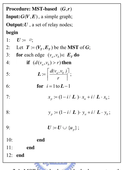
It is obvious that the resulting augmented network is connected. The description of the MST-based relay node deployment method is given in Figure

(16)

Procedure: MST-based ( rG, )

Input:G(V,E), a simple graph;

Output:U, a set of relay nodes;

begin

1: U:= ∅;

2: Let T:=(V_T,E_T)be the MST of G;

3: for each edge (va,vb)∈ETdo

4: if (d(va,vb)>r)then 5: L:= ⎥⎥ ⎤ ⎢⎢ ⎡ r ) v , d(v_a _b ; 6: for i=1toL−1 7: x_p:=(1−i/ L )⋅x_a +i/ L⋅ ; x_b 8: y_p:=(1−i/ L )⋅y_a+i/ L⋅ ; y_b 9: U:= U∪{u_p}; 10: end 11: end 12: end

Figure 2-1. MST-based relay node deployment method.

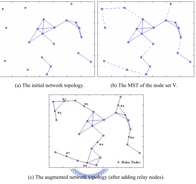
An example is given in Figure 2-2, where the solid lines are used to

indicate links in E, and dashed lines are links incident to the positions of the

relay nodes. The initial network topology is shown in Figure 2-2(a), used to build the MST (Figure 2-2(b)) of the initial network. In Figure 2-2(c) is deploying the relay nodes in the dashed lines to become the connectivity network topology.

(17)

(a) The initial network topology. (b) The MST of the node set V.

(c) The augmented network topology (after adding relay nodes).

Figure 2-2. An example of the MST-based relay node deployment method.

(a) MST-based relay node deployment (b) Two-dimension relay node deployment

(18)

The time complexity of building the MST varies from (the original Prim’s algorithm [23]) to almost linear of (the optimal algorithm [24]), where is the number of vertices and e is the number of edges. The time complexity of the rest of the algorithm is

(

e n

O log

)

e

n

( )

e

O . Therefore, the time complexity

of the MST-based method is the same as that of MST. The MST-based method will be used as baseline algorithm for comparison. Its shortcoming is, however, that each relay node can only be used to connect at most two clusters. As shown in Figure 2-3, the MST-based method would have placed 2 relay nodes to connect all three clusters, while in fact one (placed at the position of in Figure 2-3) is sufficient.

1

(19)

2.2.2 Virtual-Wiring relay node deployment method

The sensor nodes have considered their position predefined and fixed [20]. The transmission or communication range of each node, i.e., the circular range within which the message transmitted could diffuse is known. The nodes are not very powerful in terms of their communication range. The communication range of the node is limited and neighboring nodes in the vicinity alone can send and receive data packets between themselves. Establish the basic terminology, and provide the foundation concepts. The value gives the value of the length of the shortest path distance between and . One could adopt different means to generate these values but we employ matrix calculations so that a unified matrix based computations are used for the whole process.

ij

l

i

v v_j

The first step of the Virtual-Wiring (VW) relay node deployment method is

to assess the connectivity of the graph . If the graph is not a connected graph

or rather a forest, then the selected nodes in disjoint components are connected by adding a new link between them to make the whole graph connected. In reality, this is reflected in the sensor network scenario as the process of inserting new sensor nodes so that a new path of communication is resulted. Intuitively the process is explained as follows. The Network Connectivity Matrix is scanned for any

G

L

∞ entries. If there are any, it is implied that there are more than

one component that are not connected in G.

We consider the distance matrix D along with network connectivity

matrix to prioritize the pair of nodes that are to be connected. The pair with the highest priority is connected first (as explained in the following depiction) and then is updated (with new nodes and links). The new nodes inserted whose purpose is to join a particular pair may have consequential connections

L

(20)

with other neighboring nodes as well. Matrix is computed again and the

connectivity of is checked again.

L

G

To affect that action in the sensor networks scenario, we place as many new relay nodes needed to bridge the distance along the straight line between them, considering the range radius of the fixing nodes. Let us call the first pair of

nodes that are to be connected as and , where v_i v_j i and values are

obtained from the value minimum distance

j

( )

dij

min such that l_ij =∞ . By

connecting those nodes, we mean to add new relay nodes along the straight line connecting them so that they act as routers.

If we start from sensor node , then we put a new fixing sensor node in

the vicinity of the range of along the straight line between and .

a

v u_p

a

v v_a v_b

Then the position of u_p is defined in Figure 2-4.

P(up) = ( xp, yp) | xp, yp ∈ U

Where xp and yp are given by

xp = xa ± min( ra , rp )×cos

θ

and yp = ya ± min( ra , rp )×sin

θ

(± Depends on whether xa > xb or not) and

θ

= arc tan(m), where

) x x ( ) y y ( m b a b a − − =

Figure 2-4. VW relay node deployment method.

where ‘m’ is the slope of the straight line that joins the two points

(

x ,_a y_a

)

and

(

x ,b yb

)

.

An example is given in Figure 2-5, where the initial network topology is in Figure 2-5(a), used to place as many new relay nodes needed to bridge the distance along the straight line between them. In Figure 2-5(b) is deploying the

(21)

relay nodes in the disconnected link of the network connectivity matrix dependence with the minimum distance to become the connectivity network topology. However, VW relay node deployment method has drawback as the same as MST-based method that would have place 2 nodes to connect all three clusters, while in fact one placed at the position of in Figure 2-6(b) is sufficient.

1

u

(a) The initial network topology. (b) The augmented network topology. (after adding relay nodes)

Figure 2-5. An example of the VW relay node deployment method.

(a) VW relay node deployment (b) Two-dimension relay node deployment

(22)

A deployment strategy given definitions of two problems: The augmented network is connected by deploying the minimal number of additional relay nodes, and deployed relay nodes possible that the augmented network with maximum node degree. The straightforward solution is to place the relay nodes along the edges of the Euclidean MST calculated for the clusters, when the distance between two clusters is defined as the shortest distance between two terminal nodes in these distinct clusters. This can be seen by considering Kruskal’s algorithm for finding the MST [24]. The algorithm is to calculate the Euclidean MST for the initial node set, and place the relay nodes on the edges of

the MST that are longer than the transmission rang . r

The extra solution is a simple heuristic method to provide the graph connectivity, Virtual Wiring (VW) [20], that place as many new relay nodes needed to bridge the distance along the straight line between them, considering the range radius of the fixing nodes.

MST-based and VW methods will be used as baseline algorithm for comparison. Its shortcoming is, however, that each relay node can only be used to connect at most two terminal nodes. Not all necessary edges can be spanned, the better selection of edges generally requires going through all possibilities. In those case, we propose the two dimension geometric search algorithm of deploying the few additional relay nodes to improving the connectivity of exiting WSNs.

(23)

2.3 Research Objective

We aim to propose an efficient relay node deployment method to connect disconnected WSNs. To reach the purpose of reducing number of relay nodes, we propose a two dimension geometric search algorithm in order to discover a proper location where adding a single relay node results in connecting as many as possible disconnected node pairs in a given WSN. Furthermore, in order to devise a practical method, here we use the probabilistic graph model for the WSNs. This implicitly means that we assume the dominating factor affecting communications to be the path loss of radio signals coupled with radio propagation effects, including shadow fading and small-scale fading. Within this model, the transmission power employed be the sensor nodes (which we assume to be the same for all nodes), the radio propagation model, and the receiving sensitivity at reception for a desired rate of communication are woven into a single parameter, the link connectivity of a node pair, which equals to the probability that a message is correctly received from the source node to the destination node.

(24)

3. The Proposed Relay Node Deployment Method

The proposed method is composed of 5 major processes. Firstly, the link connectivity of each node pair is estimated from Initialization and Link

Connectivity Estimation processes. Then, the topology and disconnected node

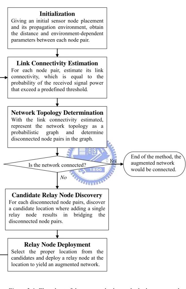
pairs of the initial network are determined in Network Topology Determination process. When the network is disconnected, the Relay Node Deployment process places a relay node in order to bridge one or more disconnected node pairs each time, where the location of the relay node is chosen from several alternatives that is discovered by Candidate Relay Nodes Discovery process. The processing flow repeats until the augmented network is connected. The flowchart of the proposed relay node deployment is given in Figure 3-1. In the following paragraphs, we elaborate on the procedure in the proposed method.

(25)

Initialization

Giving an initial sensor node placement and its propagation environment, obtain the distance and environment-dependent parameters between each node pair.

Link Connectivity Estimation

For each node pair, estimate its link connectivity, which is equal to the probability of the received signal power that exceed a predefined threshold.

Network Topology Determination

With the link connectivity estimated, represent the network topology as a probabilistic graph and determine disconnected node pairs in the graph.

Is the network connected?

Candidate Relay Node Discovery

For each disconnected node pairs, discover a candidate location where adding a single relay node results in bridging the disconnected node pairs.

Relay Node Deployment

Select the proper location from the candidates and deploy a relay node at the location to yield an augmented network.

Yes End of the method, the _{augmented network}

would be connected.

No

(26)

3.1 Link Connectivity Estimation

In order to devise a practical relay node deployment method, a realistic model for link connectivity estimation is proposed [25]. In this model, the link

connectivity of the link from node i to node , j l

( )

i, j =s_ij, is equal to the

probability of the received signal power P_R

( )

i, j (dBm) which exceed a

threshold value δ , the receiving sensitivity of sensor node. Here the link

connectivity sij is given by

( )

{

( )

}

_{( )}

_⎟⎟ ⎠ ⎞ ⎜⎜ ⎝ ⎛ − = > = = j i P j i P s j i l R R ij , exp , Pr , δ δ (1)

where is represent by a continuous random variable which takes into

account radio propagation effects, including the large-scale path loss, shadow fading, and small-scale fading. The

(

i j P_R ,

)

( )

i j P_R , is given by

( )

i j =P

( )

i j −

[

PL

( )

d +

_∑

PAF+

(

R−R

)

]

P_R , _T , _ij (2) where

(

i j

PT ,

)

denotes the transmitted signal power (dBm) from node i to node , j

( )

dij

PL represents the large-scale path loss (dB) with propagation distance

and is equal to ij d

( )

_⎟⎟ ⎠ ⎞ ⎜⎜ ⎝ ⎛ + = 0 0 10 log d d n d PL d PL _ij ij (3) where

(

d

(27)

n is the path loss exponent,

ij

d is propagation distance (m) from node i to node . j

∑

PAF represents the power attenuation (dB) due to shadow fading and is equal

to

∑

∈ ⋅ T t t t PAF N ₍₄₎ where

is the number of obstacles,

t

N

is the partition loss (dB) of an obstacle.

t

PAF

R

R− denotes a zero-mean Rayleigh distribution random variable which

represents the small-scale fading effects.

It is noted that the path loss exponents n, the path loss of reference

distance , and the shadowing fading

(

d0

PL

)

0

d

∑

PAF should be made adaptive to the

propagation environment (which is determined in the Initialization process in the proposed method). Here we made sufficient field test in the applied environment to derive the environment-dependent parameters. Table 3-1 depicts

the obtained value of the parameters from field test at 9th floor of Engineering

Building 4, National Chiao Tung University. Then, these parameters are adaptively assigned while deploying the relay nodes.

(28)

Table 3-1. The obtained value of the parameters from field test at 9th floor of Engineering Building 4, National Chiao Tung University.

Channel Parameters Value Obtained

δ Receiving Sensitivity (dBm) -89.5

T

P Transmitter Power (dBm) -35.5

( )

d0

PL Path Loss ( ) (dB) d₀ 15 (avg.)

n Path Loss Exponent 1.8~3

P

PAF A plasterboard loss (dB) 5~9

B

PAF A brick wall loss (dB) 7~15

C

(29)

3.2 Network Topology Determination

Based on the estimated link connectivity of each node pairs, the network topology would be represented by a probabilistic graph. Figure 3-3 depicts an example of the determined network topology. In order to estimate the quality of the determined topology, the best route of each node pair, the multi-hop route with maximum transmission probability, is discovered by using an All-Pairs

Strongest Path Search Algorithm that modified from known all-pairs shortest path search algorithm [26]. The maximum transmission probability of a

node pair is given by

ij w

(

i, j

)

( ) _⎭⎬ ⎫ ⎩ ⎨ ⎧ =

∏

∈ ∈ ∀ p b a ab P p ij s w ij _, max (5) where

p is a set of node pairs that forms a multihop route,

ij

P the route set formed by all available route with source node and

destination node .

a

b

A network is connected if each node can find a multi-hop route to communicate with any other node in the network. Here we consider the node

pair as being neighbors if and only if its link connectivity is larger than

a threshold value

(

i, j

)

s_ij

λ. Assuming that the route represents the best route of

node pairs , if there exists a link

ij

q

(

i, j

)

( )

c,d in q_ij whose link connectivity

λ <

cd

s , we define the node pair

( )

i, j is disconnected node pair and belongs to

the disconnected set . As a result, a network topology with empty set implies that the whole network is connected. Otherwise, more relay nodes are required in order to bridge disconnected node pairs.

(30)

3.3 Candidate Relay Node Discovery

In this process, candidate locations for relay node deployment are discovered. The stricter requirement that a single relay node should, when possible, connect more than one disconnected node pair in as potential locations of relay node placement. Here a two dimension geometric search algorithm is proposed to find out a proper location for connecting a given disconnected node pair. The search method has the following steps:

D

step 1. For a given disconnected node pair

( )

i, j in D, determine all feasible

locations of relay node placement for connecting node pair

( )

i, j . These

locations form an area A in the plane.

step 2. Find the location in A where adding a single relay node results in

connecting the largest number of disconnected node pairs in D.

step 3. If there are more than one feasible locations in step 2, select the location where adding a relay node results in connecting the largest number of neighboring nodes.

step 4. If there are more than one feasible locations in step 3, select the location where adding a relay node yields the maximal rms value of link connectivity between the node α and its neighboring nodes.

step 5. The proper location for connecting node pair

( )

i, j is discovered in step

4 and is regarded as a candidate location for relay node deployment.

Repeating the previous steps for each disconnected node pair in would results in multiple candidate locations for relay node deployment. Figure 3-2 depicts an example of Candidate Relay Node Discovery.

(31)

(32)

3.4 Relay Node Deployment

Since only one relay node is deployed in each round of proposed method, the best location for relay node deployment should be selected from candidate locations discovered by previous process. Here we consider similar criteria in

Candidate Relay Node Discovery process to determine the best candidate:

step 1. Select the candidate location where deploying a single relay node can

connect maximal number of disconnected node pairs in D.

step 2. From step 1, if multiple candidates are available, select the candidate location where can be used to connect most number of neighboring nodes. step 3. From step 2, if multiple candidates are still available, select the

candidate location, which yields the maximal rms value of link connectivity between the relay node and its neighboring nodes.

step 4. The proper candidate is selected in step 3. Adding a relay node at the selected location and go back to Link Connectivity Estimation process.

Figure 3-3 depicts an example of candidate selection from Figure 3-2. Due to is the best candidate that can solve three disconnected node pairs in , it would be select to deploy in the WSN. By repeating the process flow of the method, the connectivity of initial network is improved by deploying additional relay nodes and thereafter the network would be connected. An example of proposed relay node deployment method is given in Figure 3-4, where the initial network topology is the same as that in Figure 2-2(a) and Figure 2-5(a). By examining the example, the proposed method deploys 7 relay nodes for connecting the initial WSN, while both MST-based and VW methods require 8 relay nodes.

1

(33)

Figure 3-3. The is the best candidate that can solve three disconnected node pairs in Figure 3-2.

1

C

The proposed method would select the node to deploy in the WSN.

(a) The initial network topology. (b) The augmented network topology. (after adding relay nodes)

(34)

4. Simulation Results and Comparison

In order to evaluate the performance of our work, we present and analyze the simulation results from applying the proposed relay node deployment method for connecting randomly and uniformly distributed initial nodes in a square-shaped plane. For comparison, related works, including MST-based and VW node deployment method are also evaluated. These methods are implemented and simulated by using the MATLAB toolboxes [27].

To include the random characteristics of radio propagation channels, the propagation model shown in Eq.(2) is used to determine the augmented network by applying methods. Three types of propagation environments are considered. They are Line-Of-Sight (LOS), Non-Line-Of-Sight (NLOS) with obstacles, and NLOS with obstacles and small-scale fading. The assigned values of environment-dependent parameters in our simulation are listed in Table 4-1, which are derived from our field tests in indoor environment.

(35)

Table 4-1. The assigned values of environment-dependent parameters in our simulation.

(a) The LOS environments.

Input parameters (unit) Value assigned

LOS

D Maximum Transmission Distance of

UDM (m) 36.3

T

( )

d0

n Path Loss Exponent 2.5

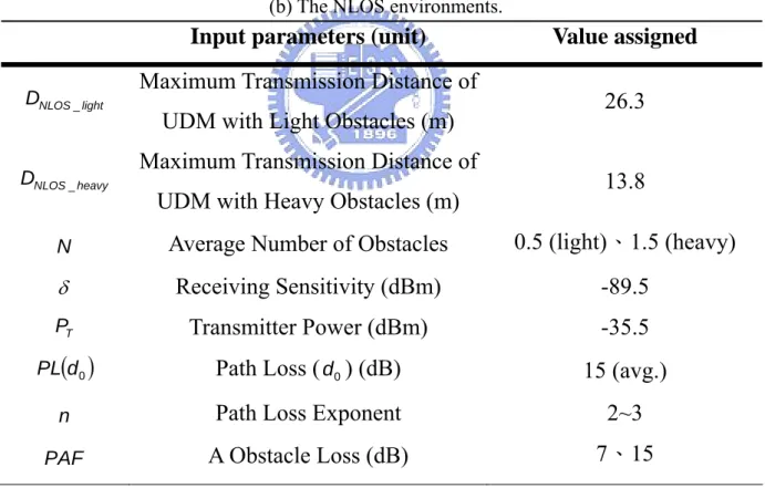
(b) The NLOS environments.

Input parameters (unit) Value assigned

light NLOS _

UDM with Light Obstacles (m) 26.3

heavy NLOS _

UDM with Heavy Obstacles (m) 13.8

N Average Number of Obstacles 0.5 (light)、1.5 (heavy)

T

( )

d0

n Path Loss Exponent 2~3

PAF A Obstacle Loss (dB) 7、15

Here, effects of node-density and topology-size on performance metrics are investigated. Each obtained data point is an average of 200 simulation runs.

(36)

4.1 Performance Metrics

Three of significant metrics are considered in order to determine the performance of the relay node deployment methods in our simulations.

(1) Average Number of Relay Nodes

Average Number of Relay Nodes (ANRN) is defined as the average of all sampled number of relay nodes deployed by an adopting method. The less the relay nodes are required to connect a disconnected WSN, the more efficient the method would be. For comparison purpose, we further examine the improvement ratio of ANRN, which is defined as

(

)

B method ng usi ANRN A and B method between ANRN of difference B A, = ρ ₍₆₎

where method B denotes a benchmark method. Here we consider the performance of MST-based method as a benchmark for the proposed method. (2) Average Node Degree

The Average Node Degree (AND) is defined as the average of all sampled node degree by an adopting method, where the node degree is defined as the average number of neighbors of all nodes in a WSN. The node degree of a WSN is strongly correlated with network connectivity [10]. The higher the node degree, the better the network connectivity would be.

(37)

(3) Average Number of Network Clusters

Average Number of Network Clusters (ANNC) is defined as average number of network clusters of augmented network by an adopting method, where a network cluster represents a portion of a network formed by a group of connected nodes. It is noted that the number of network cluster is equal to 1 when the network is connected. All of investigated relay node deployment methods aim to construct a connected WSN, however, the augmented network might be still disconnected when the chosen method is inadequate in the application/environment context. The larger the network cluster, the worse the network connectivity would be.

(38)

4.2 Node Density Effect

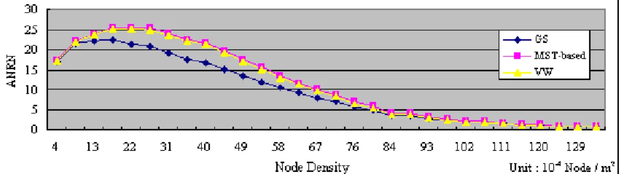
In this simulation, the performance with varying node density using each of the investigating method is evaluated. The size of operational region is considered:

150m×150m. In each simulation run, all initial nodes are uniformly distributed

in the confined region. We vary the number of initial nodes in the region from 10 to 300 that results in the increasing of node density. First of all, the simulation results obtained in LOS environment are present. Figure 4-1 and Figure 4-2 show the ANRN and improvement ratio of ANRN, respectively, of the proposed GS method comparing with that of MST-based and VW method.

Figure 4-1. ANRN versus node density in LOS environment.

Figure 4-2. Improvement ratio of ANRN versus node density in LOS environment.

(39)

By examining Figure 4-1 and Figure 4-2, the proposed GS method always yields minimum number of relay nodes. It is found that the improvement ratios

of ANRN, ρ, by using GS method are larger than 10% when the node density is

in the region of 0.002~0.011 nodes/m2. With the node density of initial network

increases, all of evaluated methods yield a small ANRN that tend to be 0. This phenomenon is due to the nature that a WSN with a higher node density is allocated, the larger the probability that the WSN would be connected. It is also shown in [10]. By summarizing the simulation results, the GS method improves 14.41% and 10.1% of ANRN comparing to MST-based and VW method,

respectively, when the sensor nodes are placed in a 150×150 m2 square region.

Figure 4-3 depicts the AND of the proposed GS method comparing with that of MST-based and VW method. It is shown that the GS method provides higher node degree comparing to other method when the node density is less

than 0.008 nodes/m2. However, with the node density increasing, the obtained

ANDs are also increasing and all of evaluated method provide equivalent ANDs.

(40)

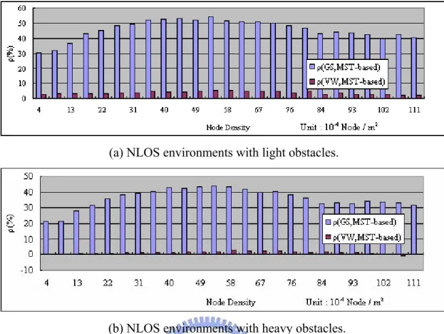
Thereafter, the simulation results obtained in NLOS environment are present. Figure 4-4 and Figure 4-5 show the ANRN and improvement ratio of ANRN, respectively, when the partition loss of an obstacle is set as 7 dB. By examining the simulation results, the proposed GS method always yields best performance in ANRN. By comparing Figure 4-2 and Figure 4-5, the proposed method provides better improvements in NLOS than in LOS, which indicates that the method is practical for applying in indoor environment. It is found that the more light the obstacles, the better the improvement by using GS method would be obtained. The averaged improvement ratios by using GS method are 45.8% and 35.8% with light obstacles and heavy obstacles, respectively.

(a) NLOS environments with light obstacles.

(b) NLOS environments with heavy obstacles.

Figure 4-4. ANRN versus node density in NLOS environment. (The partition loss of an obstacle is 7dB).

(41)

Figure 4-5. Improvement ratio of ANRN versus node density in NLOS environment. (The partition loss of an obstacle is 7dB).

Figure 4-6 depicts the AND of the proposed GS method comparing with that of MST-based and VW method in NLOS environment. It is shown that the GS method significantly improves the performance of ANRN while at the same time provides equivalent or slightly smaller node degree comparing to other method.

(42)

Figure 4-6. AND versus number of nodes in NLOS environment. (The partition loss of an obstacle is 7dB).

Figure 4-7 and Figure 4-8 show the ANRN and improvement ratio of ANRN, respectively, when the partition loss of an obstacle is set as 15dB. By comparing the NLOS cases when the partition loss of an obstacle is set as 7dB, analogous results are obtained. Here the averaged improvement ratios by using GS method are 25.4% and 20.6% with light obstacles and heavy obstacles, respectively, which are slightly smaller than the results in NLOS environment when the partition loss of an obstacle is set as 7dB.

(43)

Figure 4-7. ANRN versus node density in NLOS environment. (The partition loss of an obstacle is 15dB).

Figure 4-8. Improvement ratio of ANRN versus node density in NLOS environment. (The partition loss of an obstacle is 15dB).

(44)

(a) Environments with light obstacles.

(b) Environments with heavy obstacles.

Figure 4-9. AND versus number of nodes in NLOS environment. (The partition loss of an obstacle is 15dB).

As to the ANNC by using each of the methods in NLOS environment, the proposed GS method always provides connected WSNs after deploying relay nodes. On the other hand, both MST-based and VW method might be inadequate in NLOS environment, especially when the obstacles are heavy. The evidence is showed in Figure 4-10.

(45)

(a) NLOS environments with light obstacles (7dB).

(b) NLOS environments with light obstacles (15dB).

(c) NLOS environments with heavy obstacles (7dB).

(d) NLOS environments with heavy obstacles (15dB).

(46)

Simulation results obtained in NLOS environment with small-scale fading effect are present in the following figures. Figure 4-11 and Figure 4-12 show the ANRN and improvement ratio of ANRN, respectively, which yield similar curves comparing to Figure 4-4 and Figure 4-5. The average improvement ratios of ANRN are 38% and 29.9% with light obstacles and heavy obstacles, respectively. It is noted that the improvement ratios are slightly larger than prior results, which indicates that the proposed method is adequate in indoor environment, especially when the small-scale fading effect is considered. Figure 4-13 and Figure 4-14 depict the AND and ANNC, respectively, of the proposed

GS method comparing with that of MST-based and VWmethod. It is shown that

the GS slightly decreases node degree but always provides connected WSNs after deploying relay nodes.

(47)

(a) NLOS environments with light obstacles and small-scale fading (7dB).

(b) NLOS environments with light obstacles and small-scale fading (15dB).

(c) NLOS environments with heavy obstacles and small-scale fading (7dB).

(d) NLOS environments with heavy obstacles and small-scale fading (15dB).

Figure 4-11. ANRN versus node density in NLOS environment with small-scale fading.

(48)

Figure 4-12. Improvement ratio of ANRN versus node density in NLOS environment with small-scale fading.

(49)

Figure 4-13. AND versus number of nodes in NLOS environment with small-scale fading.

(50)

Figure 4-14. ANNC versus node density in NLOS environment with small-scale fading.

(51)

4.3 Topology Size Effect

Here, the topology size is defined as the number of initial nodes. In each simulation run, all initial nodes are uniformly distributed in an square area with

associated size. A constant node density is kept and it is equal to 1/250 nodes/m2.

We vary the number of initial nodes in the region from 10 to 200 that results in the increasing of topology size. First of all, the simulation results obtained in LOS environment are present. Figure 4-15 and Figure 4-16 show the ANRN and improvement ratio of ANRN, respectively, of the proposed GS method comparing with that of MST-based and VW method.

Figure 4-15. ANRN versus number of initial nodes in LOS environment.

Figure 4-16. Improvement radio of ANRN versus number of initial nodes in LOS environment.

(52)

By examining Figure 4-15 and Figure 4-16, the proposed GS method yields the minimum number of relay nodes in all of investigated topology sizes. It is

found that the obtained improvement ratios ρ by using GS method are tend to

converge to a constant. This phenomenon indicates that the complexity of the problem increases linearly with the increasing of topology size, and the proposed method is expected to be scalable when the topology size is large. With the topology size increases, improvement ratios are scattered in a confined range of 20%~25% and the GS method improves 22.5% and 20.3% of ANRN comparing to MST-based and VW method, respectively.

Figure 4-17 depicts the AND of the proposed GS method comparing with that of MST-based and VW method. It is shown that the GS method provides almost equivalent node degree comparing to MST-based method, while the VW method always provides worst node degree. The AND converges to a constant as about 3.05 with the increasing of topology size.

(53)

Thereafter, the simulation results versus topology sizes obtained in NLOS environment are present. Figure 4-18 and Figure 4-19 show the ANRN and improvement ratio of ANRN, respectively. The less the obstacles, the better the improvement by using GS method would be obtained. Here the proposed GS method always yields best ANRNs. Their improvement ratios are about 52.7%

and 41.6% with light obstacles and heavy obstacles, respectively, when the

partition loss of an obstacle is set as 7dB. (They are about 32.9% and 27.2%

with light obstacles and heavy obstacles, respectively, when the partition loss of an obstacle is set as 15dB.) It is found that the proposed method provides better improvements in NLOS than in LOS in most of topology sizes. An analogous phenomenon is observed when we investigation node density effect on ANRN in previous section.

(54)

(55)

Figure 4-19. Improvement ratio of ANRN versus number of initial nodes in NLOS environment.

(56)

Figure 4-20 depicts the AND versus topology sizes by using all the investigated methods in NLOS environment. Due to the nature that the more nodes placed in a confined area results in higher node degree, the obtained ANDs by using either MST-based method or VW method are slightly larger than the ANDs obtained by proposed method. However, the proposed GS method always provides connected WSNs even in a smaller AND. The evidence is showed that the obtained ANNCs of proposed method are equal to 1 in Figure 4-21.

(57)

(58)

(59)

Furthermore, the simulation results obtained in NLOS environment with small-scale fading effect are present in the following figures. Figure 4-22 and Figure 4-23 show the ANRN and improvement ratio of ANRN, respectively. The

average improvement ratios of ANRN are 48.95% and 31.9% with light

obstacles and heavy obstacles, respectively. It is also found that the improvement ratios are slightly larger than prior results in Figure 4-19. Figure 4-24 and Figure 4-25 depict the AND and ANNC, respectively. It is shown that the GS has less AND than other methods, but always provides connected WSNs after deploying relay nodes.

(60)

(61)

Figure 4-23. Improvement ratio of ANRN versus number of initial nodes in NLOS environment.

(62)

(63)

(a) NLOS environments with light obstacles and small-scale fading ( 7 dB).

(b) NLOS environments with light obstacles and small-scale fading ( 15 dB).

(c) NLOS environments with heavy obstacles and small-scale fading ( 7 dB).

(d) NLOS environments with heavy obstacles and small-scale fading ( 15 dB).

(64)

5. Conclusion

In this research, we propose a relay node deployment method, named as Greedy-Search (GS) method, for placing additional relay nodes to improve the network connectivity of disconnected WSNs. By using a geometric search algorithm, every relay node is placed at a proper location, which results in significant reducing the number of required relay nodes. Besides, by considering radio propagation effect, a realistic model for estimating the connectivity of a radio link is proposed, which yields accurate network topology determination especially for applying the method in indoor environment. Simulation results prove that the proposed method has the best performance in average number of relay nodes comparing to related works. It is found that the proposed method provides significant improvements on ANRN comparing to related works, when

the node density is in the region of 0.002~0.011 nodes/m2. The average

improvement ratio of ANRN is 22.5%, 38.6%, and 40.9%, in LOS, NLOS with obstacles, NLOS with obstacles and small-scale fading, respectively, when the

node density is equal to 1/250 nodes/m2. It indicates that there are about 20% of

improvement contributed by the proposed two dimension geometric search algorithm, and about 30% of improvement due to the accurately determining of network topology by using the proposed link connectivity estimation model. Due to the proposed method significantly reduces the number of relay nodes, it slightly decrease node degree comparing to the MST-based and VW methods. However, by examining the obtained ANNCs, the proposed method always provides connected WSNs after deploying relay nodes, especially in NLOS environment with heavy obstacles. Above all, the proposed method is an effective and efficient method for relay node deployment.

(65)

References

[1] K. Romer, F. Mattern, “The Design Space of Wireless Sensor Networks”, IEEE Wireless

Communications, vol.11, issue.6, pp. 54-61, Dec. 2004

[2] T. Haenselmann, Sensornetworks, GFDL Wireless Sensor Network textbook. Retrieved on 2006

[3] M. Tubaishat and S. Madria, “Sensor networks: an overview”, IEEE Potentials, vol. 22, issue 2, pp. 20–23, April-May 2003

[4] Santi, Paolo, “Topology control in wireless ad hoc and sensor networks”, ACM

Computing Surveys (CSUR), vol. 37, issue 2, pp. 164-194, 2006

[5] Bhaskar Krishnamachari, Networking Wireless Sensors, Cambridge University Press, January 2006

[6] K. Fadila, S.-R. David; “Connectivity and Topology Control in Wireless Ad Hoc Networks with Realistic Physical Layer”, ICWMC '07. Third International Conference, pp. 49 – 49, March 2007

[7] P. Gupta, P.R. Kumar, “Critical power for asymptotic connectivity in wireless networks”,

In Stochastic analysis, control, optimization and applications: a volume in honor, 1998

[8] P.J. Wan and C. W. Yi, “Asymptotic critical transmission radius and critical neighbor number for κ-connectivity in wireless ad hoc network”, In Proc. 5th ACM Symposium on

Mobile Ad Hoc Networking and Computing (MOBIHOC), Roppongi, Japan, May 2004

[9] F. Xue, P.R. Kumar, “The number of neighbors needed for connectivity of wireless networks”, Wireless Networks, 10(2), pp. 169–181, Mar. 2004

[10] C. Bettstetter, “On the minimum node degree and connectivity of a wireless multihop network”, in Proc. 3rd ACM International Symposium on Mobile Ad Hoc Networking &

Computing, pp. 80–91, 2002

[11] V. Isler, S. Kannan, K. Daniilidis, “Sampling Based Sensor-Network Deployment”,

Intelligent Robots and Systems (IROS), 2004

[12] S. Kumar, T.H. Lai, J. Balogh, “On κ-Coverage in a Mostly Sleeping Sensor Network”,

in ACM MobiCom’04, 2004

[13] G. Xing, C. Lu, R. Pless, J.A. O’Sullivan, “Co-Grid: an Efficient Coverage Maintenance Protocol for Distributed Sensor Networks”, in Information Proceesing in Sensor

Network (IPSN’04), 2004

[14] C.F. Huang, Y.C. Tseng, “The Coverage Problem in a Wireless Sensor Network”, in

(66)

[15] X. Wang, G. Xing, Y. Zhang, C. Lu, R. Pless, C. Gill, “Integrated Coverage and Connectivity Configuration in Wireless Sensor Networks”, in Proceedings of ACM

SenSys, pp. 28-39, Los Angeles、CA, 2003

[16] T. Yan, T. He, J.A. Stankovic, “Differentiated Surveillance for Sensor Networks”, in

Proceedings of ACM SenSys, pp. 51-62, Los Angeles、CA, 2003

[17] M. D. Penrose, “The longest edge of random minimal spanning tree”, Annals of Applied

Probability, 7(2), pp. 340–361, 1997

[18] N. Li, J.C. Hou, “FLSS: A fault-tolerant topology control algorithm for wireless networks”, In Proc. 10th ACM International Conference on Mobile Computing and

Networking (MOBICOM), pp. 275–286, Philadelphia、USA, Sept. 2004

[19] I. Stojmenovic, A. Nayak, J. Kuruvila, “Design guidelines for routing protocols in ad hoc and sensor networks with a realistic physical layer”, In Communications Magazine,

IEEE, vol. 43, pp. 101–106, March 2005

[20] M.K.Vairamuthu, S. Nesamony, M.E. Orlowska, and S.W. Sadiq, “On the Design Issues of Wireless Sensor Networks for Telemetry”, Database and Expert Systems Applications, 2005

[21] M. Audeh, “Metropolitan-scale Wi-Fi mesh networks”, Computer, 2004

[22] N. Li, J.C. Hou, “Improving connectivity of wireless ad hoc networks”, MobiQuitous,

The Second Annual International Conference, pp. 314 – 324, on 17-21 July 2005

[23] R. Prim., “Shortest connection networks and some generalizations”, The Bell System

Technical Journal, 36, pp. 1389–1957, 1957

[24] S. Pettie, V. Ramachandran., “An optimal minimum spanning tree algorithm”, Journal of

the ACM, 49(1), pp. 16–34, Jan. 2002

[25] Theodore S. Rappaport, Wireless Communications - principles and practice, second Edition, Prentice Hall Communications Engineering and Emerging Technologies Series, 2002

[26] T.H. Cormen, C.E. Leiserson, R.L. Rivest, INTRODUCTION TO ALGORITHMS, Eleventh printing, the MIT Press Cambridge, Massachusetts London, England, 1994 [27] Math Works, http://www.mathworks.com

[28] P. Gupta, P. Kumar, “The capacity of wireless networks”, IEEE Trans. Inform. Theory, vol. 46, pp. 388–404, March 2000

[29] C. Bettstetter, C. Hartmann, “Connectivity of wireless multihop networks in a shadow fading environment”, in Proc. 6th ACM International Workshop on Modeling, Analysis

and Simulation of Wireless and Mobile Systems, pp. 28–32, 2003

[30] C. Foh, B. Lee, “A closed form network connectivity formula for one-dimensional MANETs”, in Proc. IEEE ICC 2004, vol. 6, pp. 3739–3742, June 2004

[31] C. Foh, G. Liu, B. Lee, B. Seet, K. Wong, and C. Fu, “Network connectivity of one-dimensional MANETs with random waypoint movement”, IEEE Commun. Lett., vol.

(67)

[32] R. Sedgewick, Algorithms in C, Addison Wesley, 1990

[33] 鄭錦聰編著, MATLAB程式設計基礎篇, 全華科技圖書股份有限公司, 2001 [34] 莊鎮嘉,鄭錦聰編著, MATLAB程式設計實務, 全華科技圖書股份有限公司, 2006 [35] 洪維恩著, Matlab7程式設計, 旗標出版股份有限公司, 2006

無線感測網路中繼節點佈建方法之研發-以室內環境為例

國

立

交

通

大

學

電機學院 IC 設計產業研發碩士班

碩

士

論

文

無線感測網路中繼節點佈建方法之研發-以室內環境為例

Development of a Relay Node Deployment Method for Disconnected Wireless

Sensor Networks: Applied in Indoor Environments

研 究 生：劉蓓縝

指 導 教 授：唐震寰 教授

無線感測網路中繼節點佈建方法之研發-以室內環境為例

Development of a Relay Node Deployment Method for Disconnected Wireless

Sensor Networks: Applied in Indoor Environments

無線感測網路中繼節點佈建方法之研發-以室內環境為例

摘 要

ABSTRACT

誌 謝

Contents

List of Tables

List of Figures

1. Introduction

( )

(

)

( )

( )

(

)

2. Problem Definition and Related Works

2.1 Problem Definition

(

)

{

}

{

( ) ( )

}

( )

( )

{

}

(

) (

)

{

( ) ( )

}

2.2 Related Works

(

)

( )

( )

θ

θ

θ

(

)

(

)

2.3 Research Objective

3. The Proposed Relay Node Deployment Method

3.1 Link Connectivity Estimation

( )

( )

( )

{

( )

}

( )

(

)

( )

( )

研究生：劉蓓縝

指導教授：唐震寰教授

摘要

誌謝

_{( )}

_∑