An Effective Algorithm for Mining Association Rules with Multiple Thresholds

全文

(1)An Effective Algorithm for Mining Association Rules with Multiple Thresholds Yi Siou Lin, Kun Yuan Chang, Cheng Chen Institute of Computer Science and Information Engineering National Chiao Tung University, Hsinchu, Taiwan, R.O.C. Email:{linys, kychang, cchen}@csie.nctu.edu.tw Tel: +886-3-5712121 ext 54734. Abstract Catering. the. buying. Itemset, E-Commerce, Multiple Thresholds behaviors. 1. Introduction. of. customers becomes more and more important by. Recently,. with. the. popularization. the popularization of E-Commerce recently.. E-Commerce,. how. to. predict. How to find the association rules efficiently. psychology and tendency correctly becomes. from the transaction records is one of the most. more and more important [14][8]. One of the. interesting topics to be investigated. In this paper,. most interesting topics in data mining is the. at first, we propose en efficient algorithm,. problem of discovering association rules over. named Early Pruning Partition algorithm (EPP),. basket data [1][12-15]. An association rule. with. consists. extending. the. concept. of. Partition. of. two. subsets,. of. consumer. antecedent. and. algorithm and using an early pruning technology. consequent, such that each subset may include. to improve the performance of mining frequent. several items. And these two subsets apply to an. itemsets under single minimum support. Then. implied relation [6]. The possibility of this. we add the checking of multiple thresholds in. situation is the confidence of this association rule. EPP algorithm to construct our Multiple. [1][2][6].. Thresholds Early Pruning Partition algorithm. recommendations from association rules. The. (MTEPP). Our MTEPP algorithm can find more. search of frequent itemsets is one of the most. effective frequent itemsets corresponding to. important procedures of discovering association. some events of buying behavior. For evaluating. rules. How to develop an algorithm to gather. our algorithm, we also implement a simulation. frequent itemsets quickly is quite meaningful.. We. can. generate. some. environment to verify it. According to our. We use an early pruning technique to. evaluations, our algorithms outperform than that. construct our Early Pruning Partition algorithm. of previous methods and find the more useful. (EPP). It is based on the concept of Partition. frequent. detailed. algorithm. embedded. descriptions of our algorithms will be given in. technique. to. achieve. the contents.. However,. if. there. itemsets. indeed.. The. with. are. early. better many. pruning. performance. the. same. transactions generated suddenly in a short time. Keywords. interval such as a week or a month and then. Data Mining, Association Rules, Frequent. disappear, which is called sudden event,.

(2) traditional single threshold algorithms are not. The. suitable to solve this case. To aim at this. transactions in D containing X. A rule has a. weakness, we add the checking of multiple. measure of its strength called the confidence,. thresholds in EPP to construct the Multiple. where confidence(X ⇒ Y) = support(X ∪. Thresholds Early Pruning Partition algorithm. Y)/support(X) .. support(X). equals. the. fraction. of. (MTEPP). Our EPP algorithm outperforms at. The problem of mining association rules is. most 37% than that of Apriori algorithm and. to find all the association rules of the form X ⇒. 13% than that of Partition algorithm from the. Y that satisfy the following two conditions,. simulation results. Comparing with the total. support(X ∪ Y) ≥ minsup and confidence(X ⇒. execution. algorithm. Y) ≥ minconf. Here, minsup and minconf are. outperforms averagely 50% than that of Apriori. user specified thresholds. All itemsets that have. algorithm and 28% than that of Partition. support above the user specified minimum. algorithm.. support are generated. These itemsets are called. time,. our. MTEPP. The remaining part of our paper is organized. the large itemsets (or frequent itemsets). For. as follows. In section 2, we give a formal. each large itemset X and any Y ⊂ X, check if. description of discovering frequent itemsets. rule (X-Y) ⇒ Y has confidence above minconf.. problem and give an overview of the previous. These rules are called the strong rules.. algorithms. In section 3, we describe early. Generating. pruning technology and our EPP algorithm in. frequent itemsets is relatively straightforward.. some detail. The benefits of using multiple. However, finding all frequent itemsets is. thresholds and our MTEPP algorithm are. nontrivial if the size of the set of items, | I |, and. described in section 4. In section 5, our. the database, D, are large. We can conclude two. simulation environment is introduced and some. following properties by observation:. preliminary evaluations of our algorithms are. 1.. collected and compared with other previous. association. from. Any subset of a frequent itemset must. (2.1-1) 2.. Any superset of an infrequent itemset must also be infrequent.. 2. Background and Related Work 2.1 Problem Description [1-3] [6-7]. rules. also be frequent.. methods. Finally, some concluding remarks are given in section 6.. strong. (2.1-2). In the following subsections, we will introduce some basic algorithms based on the. Let I={i1, i2,…, im} be a set of literals called. above problem description. For easy description,. items. Let D be a set of transactions. Each. we usually notate the set of the frequent. transaction T contains a set of items ii, ij,…, ik ⊂. k-itemsets as Lk and the set of the candidate. I. An association rule is an implication of the. k-itemsets as Ck.. form X ⇒ Y, where X,Y ⊂ I , X ∩ Y = ∅. A set. 2.2 Apriori Algorithm [1][2]. of items is called an itemset. An itemset with k. Apriori algorithm is one of the most. items in it is referred to as k-itemset. Each. important level-wise algorithms for discovering. itemset X ⊂ I has a measurement called support.. frequent. itemsets.. Items. are. sorted. in.

(3) lexicographic order. Frequent itemsets are. counters for each global candidate itemset and. computed iteratively in the ascending order of. counts their support in all n partitions. It outputs. size. Assume the largest frequent itemsets. global large itemsets that have the minimum. contain k items, it takes k iterations for mining. global support along with their support. Unlike. all frequent itemsets. Initial iteration computes. the Apriori algorithm, the Partition algorithm. the frequent 1-itemsets L1. Then, for each. just needs scan the entire database twice. Thus,. iteration i≤ k, all frequent i-itemsets are. we will adopt the principle of Partition algorithm. computed by scanning database once. Iteration i. combined with early pruning technique to. consists of two phases. First, the set Ci of. develop a more efficient method, called EPP, and. candidate i-itemsets are created by joining the. then extend it to handle multiple thresholds with. frequent (i-1)-itemsets in Li-1 found in the. mining association rules. In the following, we. previous iteration. Next, the database is scanned. will describe them in some detail.. for determining the support of all candidates in Ci and the frequent i-itemsets Li are extracted from these candidates. This iteration is repeated. 3. Early Pruning Partition algorithm 3.1 Early Local Pruning [9]. until no more candidates can be generated. The. The idea of early local pruning is as. Apriori algorithm needs to take k database. follows. When reading a partition pi to generate. passes to generate all frequent itemsets. For disk. Lpi1, we record and accumulate the number of. resident databases, this requires reading the. occurrences for each item. Thus, after reading. database completely for each pass resulting in a. partition pi, we know both the number of. large number of disk reads. It means that the. occurrences for each item in partition pi, and the. Apriori algorithm takes a huge I/O operations.. number of occurrences for each item in the big. This is the major weakness of it.. partition ∪j=1,2,…,i pj denoted by BP1…i . With. 2.3 Partition Algorithm [12][10]. this information, we can get frequent 1-itemsets. The Partition algorithm focuses on times. of partition pi and partition BP1…i . We define. of scanning database. Initially the database D is. Bpi1 as the set of all better local frequent. logically partitioned into n partitions. Basically. 1-itemsets in partition pi, where Bpi1 = Lpi1 ∩. the Partition algorithm can be divided into two. LBP1…i1. With early local pruning, we use Bpi1. phases. In phase I, it takes n iterations. During. instead of Lpi1 to start the level-wise algorithm to. iteration i, only partition pi is considered. Then. construct the set Bpi of all better local frequent. take a partition pi as input and generate local. itemsets in partition pi. Since the size of Bpi1 is. large itemsets of all lengths, Li2, Li3, …, Lim as. usually smaller than that of Lpi1, Bpi can be. the output. In the merge phase the local large. constructed faster than Lpi. With Partition. itemsets with the same lengths from all n. algorithm introduced before ensures that CG =. partitions are combined to generate the global. ∪i=1,2,…,n Lpi is a super set of the set LG of all. candidate itemsets. The set of global candidate. global large itemsets. With early local pruning,. G. itemsets of length j is computed as C i=1,…,n. j. = ∪. Lij . In phase II, the algorithm sets up. Lemma 1 shows that CG = ∪i=1,2,…,n Bpi is also a superset of LG..

(4) Lemma 1 Let the database D be divided into n G. pi. partition to the big partition, current partition. partitions, p1,p2,…,pn. Let C = ∪i=1,2,…,n B .. and the occurrent transaction id. Here we also. Then, CG is a superset of LG.[9]. record the length account of each transaction in. Proof: see [9].. each partition and the length account in the. 3.2 EPP algorithm. whole database. When we have read the partition. In previous subsection, we have introduced. pi completely, we generate the better frequent. the idea of early local pruning. Then we will. 1-itemsets by using early local pruning. We. describe how to combine it with Partition. collect all items which count are larger than the. algorithm. We propose a method named Early. local minimum support = minsup/n as Lpi1, and. Pruning Partition algorithm (EPP algorithm) for. check BPcount of all items with the big partition. mining frequent itemsets quickly. Figure 1 is the. minimum support = i*minsup/n. If it is larger,. complete steps of EPP algorithm. We use an. put the item into LBPi1. Then we get Bpi1 by union. array of object named “item” to keep the. Lpi1 and LBPi1.. accumulative result such that item[j] means the. After getting the better frequent 1-itemsets. item this site sold which id is equal to j. The. Bpi1, we calculate the length of local maximum. object “item” consists of three elements:. frequent transactions. Finally, we use the. BPcount, count and tidlist to stores the. procedure gen_frequent_itemset to generate all. occurrence of this item from the first reading. local frequent itemsets from Bpi1.. Algorithm EPP // Phase I 1. for i = 1 to n do begin 2. forall transaction t ∈ pi do begin 3. forall item j ∈ t do begin 4. accumulate the occurrence of item[j] 5. end 6. accumulate the local and global maximum transaction count 7. end 8. calculate the values of local minimum support and big partition support 9. generate the better local frequent 1-itemset Bpi1 of partition pi 10. calculate the length of local maximum frequent transaction M 11. Bpi = gen_frequent_itemset(M, Sup, Bpi1, item) 12. reset all local variables 13. end 14. CG’ = Bp1 ∪ Bp2 ∪ … ∪ Bpn 15. calculate the global minimum support MG 16. CG = { c ∈ CG’ | c.length ≤ MG} // Phase II 17. forall transaction t ∈ D do 18. forall subset s ∈ t do begin 19. if s ∈ CG then 20. s.count ++ 21. end 22. LG = { c ∈ CG | c.count ≥ minsup} 23. Answer = LG Figure 1. Early Pruning Partition algorithm.

(5) Procedure gen_frequent_itemset(M, Sup, Bpi1,. pi. After finishing to process all partitions in. item). phase I of EPP algorithm, we can get all better. 1. 2.. for (k=2;. ∧ k ≤ M; k++) do. Bpik≠∅. local frequent itemsets Bp1, Bp2, … Bpn of each. forall distinct itemsets l1, l2 ∈ Bpik-1 do. partition. Before joining all local frequent. if l1[1]=l2[1] ∧ … ∧ l1[k-2]=l2[k-2] ∧. 3.. itemsets, we can use the length of global maximum transactions to eliminate some useless. l1[k-1]<l2[k-1] then begin 4.. c = (l1[1], l1[2], … l1[k-1], l2[k-1]). candidates. Finally we can join all remainder. 5.. forall (k-1)-subset s of c do. candidates from Bpi to CG to get the set of global. if all s ∈ Bpik-1 then begin. 6.. candidate itemsets. Then we continue to process. 7.. c.tidlist = l1.tidlist ∩ l2.tidlist. the phase II of EPP algorithm by rescanning. 8.. if |c.tidlist| ≥ Sup then. each transaction t in the whole database D, and. Bpik. 9. 10.. =. Bpik. ∪c. checking all subsets of t. The set of all candidate itemset c whose count is larger than minsup is. end. 11.. the global frequent itemsets LG. This is the. end. 12. Bpi = Bpi1 ∪ Bpi2 ∪ … ∪ Bpik-1. output of our EPP algorithm.. pi. 13. Answer = B. We inherit the step of Partition algorithm and use. Bpi1. frequent. instead of. itemsets.. Lpi1. Here. as the level 1 we. make. an. 4. Multiple Thresholds Early Pruning Partition algorithm 4.1 Event latency. improvement, we add k ≤ M to the second term. When a new popular purchasing behavior. of “for loop”. We will not check level larger than. occurs, it implies some new association rules. M because there is no possible frequent. will be found. If this kind of behaviors will. transaction which length is larger than M. Then. disappear in a while, we call the appearance of. we use the join step of Partition algorithm to. these behaviors as event. The new association. generate all new candidate itemsets. We do some. rules will not be found until the occurrence of. check before joining these two tidlists. We check. purchasing behavior achieves the minimum. all (k-1)-subsets of c to confirm that all. support. There is latency between the first. (k-1)-subsets of c belong to better local frequent. customer bought and the new frequent itemsets. (k-1)-itemset. the. were found. We call this latency as event latency.. observation 2.1-2 we introduced in section 2.1, if. It is intuitively better to reduce the event latency. itemset j is infrequent, all superset of j is also. as short as possible because we can make some. infrequent. After joining the tidlist of c, we can. appropriate. easily compute the support of c by calculating. association rules quickly. In the previous. Bpik,. discussions of frequent itemsets, there is only. the set of better frequent k-itemset in partition pi.. one global minimum support . It is impossible to. At the end of procedure gen_frequent_itemset,. reduce the latency unless we reduce the. we join all sets of better frequent itemset in each. corresponding local minimum support. Before. of. partition. pi.. With. the length of tidlist. Finally we can calculate. pi. level to B , the better local frequent itemsets of. recommendations. from. showing how to solve this problem,. those.

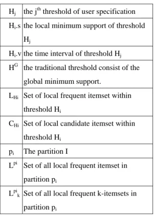
(6) Table 1 Notation Hj. th. the j threshold of user specification. Hi.s the local minimum support of threshold Hj. we first denote some symbols using in our algorithm. These symbols are listed in Table 1.We propose a multiple thresholds concept as follows. Assume that each threshold consists of. Hi.v the time interval of threshold Hj. one local minimum support and a time interval,. HG the traditional threshold consist of the. denoted by H = (s, v), where s is local minimum. global minimum support. LHi Set of local frequent itemset within threshold Hi CHi Set of local candidate itemset within. pi. support and v is time interval. For example, H1 = (10%, 30) denotes “the itemsets which appear in more than 10% of transactions happened in the last 30 days”. We can also denote HG=(minsup,. threshold Hi. total days during the store was operating) as a. The partition I. global threshold. This threshold HG is used to. Lpi Set of all local frequent itemset in partition pi Lpik Set of all local frequent k-itemsets in partition pi. filter traditional frequent itemsets within the whole database in our algorithm. And then we can use these thresholds to filter frequent itemsets. Thus, we will get several sets LH1, LH2, … LHk and LG of frequent itemsets. Algorithm MTEPP // Phase I 1. for i = n to 1 do begin 2. for t = latest transaction in pi to earliest transaction do begin 3. forall item j ∈ t do begin 4. accumulate the occurrence of item[j] 5. end 6. accumulate the local and global maximum transaction count 7. end 8. calculate the current local and big partition support by gen_current_support() 9. generate the better local frequent 1-itemset Bpi1 of partition pi 10. calculate the length of local maximum frequent transaction M 11. Bpi = gen_frequent_itemset(M, Sup, Bpi1, item) 12. reset all local variables 13. end 14. CG = Bpn ∪ Bp(n-1) ∪ … ∪ Bp1 // Phase II 15. for t = latest transaction in D to earliest transaction do begin 16. forall subset s ∈ t do 17. if s ∈ CG then 18. s.count ++ 19. if the count of reading transactions fits to |Hz.v| then 20. LHz = { c ∈ CG | c.count ≥ Hz.s } 21. end 22. LG = { c ∈ CG’ | c.count ≥ HG.s } 23. Answer = LH1, LH2, … LHh, LG Figure 2 Multiple Thresholds Early Pruning Partition algorithm.

(7) corresponding to each threshold respectively.. minimum support s1. L2 is the set of local. The newly additional association rules gathered. frequent itemsets with local minimum support s2.. from these frequent itemsets often correspond to. If s2 ≥ s1, then L2 ⊆ L1.. some events. Thus we can make more suitable. Proof:. It’s easy to prove it below. ∀ local frequent itemset t ∈ L2,. recommendations according to these rules.. t.support ≥ s2. The previous methods like Apriori and Partition algorithms can also generate the. ∵ s2 ≥ s1 ∴ t.support ≥ s1. additional association rules by run more k+1. ⇒ t ∈ L1 ⇒ L2 ⊆ L1 - Q.E.D -. times, which will be inefficient obviously.. The step of procedure get_current_minsup are. 4.2 MTEPP algorithm. described below:. In this subsection, we will describe our Multiple Thresholds Early Pruning Partition. Procedure get_current_minsup( P , i) 1.. Locate Hcur in all thresholds H1, …. algorithm (MTEPP) in some detail. Basically. Hh and HG where size of transactions. MTEPP algorithm is generalized from EPP. in Hcur-1.v < | P | ≤ size of. algorithm. In fact, EPP algorithm is a special. transactions in Hcur.v. case of MTEPP algorithm, with only one. 2.. | Hcur.v |. threshold. At first, we specify h local thresholds H1, H2, … Hh and a global threshold HG. Figure 2. H G .s |P| × (n − i + 1) ) × Hh.s , n | Hh.v |. shows the complete steps of MTEPP algorithm. Unlike the traditional algorithms like Apriori,. Sup=min( | P | × Hcur.s ,. 3.. Answer = Sup. Partition algorithm, MTEPP algorithm scans database with inverse direction, from the latest. After finding the better local frequent. transaction to the earliest transaction. While. 1-itemset Bpi1 in partition pi, we use the same. finishing to read a partition pi, we also calculate. steps as EPP algorithm to calculate the. the better local frequent 1-itemset. We use. maximum frequent transaction and then finally. another. to. compute the local frequent itemsets Bpi. Then we. compute the current local minimum support and. join all local frequent itemsets to global. current big partition minimum support. The. candidate itemsets CG and continue to process. procedure. some. phase II. In the second scan, we also reverse the. problems in supporting multiple thresholds. direction of scan. While finishing to read all. because a partition pi may be included in many. transactions specified in threshold Hi, we. thresholds. Which support of these thresholds. calculate the frequent itemsets LHi. For the. should we use to filter local frequent itemsets?. previous assumption |H1.v| < |H2.v| < … < |Hh.v|. Our solution is to use the minimum value. The. < |HG.v|, we can easily check this from H1 to Hh. reason can be explained in Lemma 2.. and HG. After reading all transactions in database. Lemma 2 Let the database D be divided into n. D, we can finally calculate the global frequent. partitions, p1,p2,…,pn. Assume in partition pi, L1. itemsets LG. The sets LH1, LH2, … LHh, LG are the. is the set of local frequent itemsets with local. final outputs of our MTEPP algorithm.. procedure. get_current_minsup. get_current_minsup. solves.

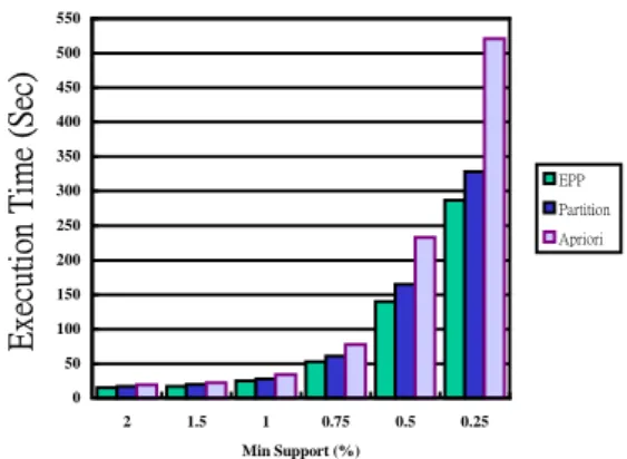
(8) 5. Simulation Environment and Table 2 Parameters of synthetic database generator. Performance Evaluation 5.1 Simulation Environment. |D| Number of transactions. The whole simulation environment is implemented in a PC with a 1000MHz AMD. |T| Average number of items per transactions |I| Average number of items of maximal potentially frequent itemsets. ThunderBird processor and 512 MB main memory. All simulation data resided on a 13 GB. |L| Number of maximal potentially frequent itemsets. IDE Ultra DMA 66 hard disk. The operating system is FreeBSD 4.3-stable. We use C++. N Number of items. language to implement and g++ compiler to. Table3 Parameters setting of our input databases. compile. Name. these. algorithms.. The. overall. |T| |I| |D|. |L|. N. Size(MB). architecture of our simulator is shown in Figure. T10.I4.D100K 10 4 100K 2000 1000. 31. 3.. T20.I2.D100K 20 2 100K 2000 1000. 63. T20.I4.D100K 20 4 100K 2000 1000. 63. T20.I6.D100K 20 6 100K 2000 1000. 63. In this subsection we will compare our EPP with Apriori and Partition algorithms. We use. two. databases,. T10.I4.D100K. and. T20.I4.D100K, to test the variation with changing minimum support. We divide the database into 10 partitions for EPP and Partition algorithms. The results for the T10.I4.D100K Figure 3 The overall architecture of our simulator The synthetic data generation procedure is. and T20.I4.D100K databases are shown in Figure 4 and Figure 5 respectively. Our EPP. described in [2], whose parameters are shown in. algorithm. Table 2. We use the generator developed by IBM. Apriori and Partition algorithm at total execution. Quest project to generate the synthetic database. time. For the case of database T10.I4.D100K,. [16]. The length of a transaction is determined. EPP algorithm outperforms Apriori from 21% to. by a Poisson distribution with mean µ to | T |.. 44.9% with minimum support of 2% to 0.25%. We have generated four different databases by. respectively. The average efficiency of EPP is. using. for. better than Apriori with 31.2%. Our EPP. performance evaluation. Table 3 shows the. algorithm is also better than Partition algorithm. names and parameter settings for each database.. with average efficiency of 12%.. 5 .2 Performance Evaluation 5.2.1 Evaluation of Single Threshold Algorithms. In the case of data base T20.I4.D100K, our EPP. the. generator. and. used. them. performs. always. more. significantly. efficient. than. outperforms. that. of. T10.I4.D100K, It outperforms Apriori with average efficiency of 32.4% and Partition.

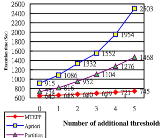
(9) and T20.I4.D100K, and set the global minimum. 550. supports as 0.5%. And then we adopt 1 to 6. Execution Time (Sec). 500 450. thresholds using in our MTEPP algorithm and. 400 350 EPP. 300. other algorithms as six conditions. The first. Partition 250. Apriori. 200. condition is just using the global threshold HG and the second condition is using H1 and HG as. 150 100. thresholds, and so on. Table 4 shows the. 50 0 2. 1.5. 1. 0.75. 0.5. parameters of these six thresholds.. 0.25. Min Support (%). The evaluation result is illustrated in Figure 6 and. Figure 4 The execution time of database T10.I4.D100k. Figure. 7. corresponding. to. database. T10.I4.D100K and T20.I4.D100K respectively. Execution Time (Sec). 2200. When the number of thresholds increases, the. 2000. total execution time of all algorithms grows. In. 1800 1600 1400 EPP. 1200. Partition 1000. Apriori. the case of input database as T10.I4.D100K, our MTEPP algorithm outperforms 39.9% to 60.3%. 800. than that of Apriori algorithm, the average value. 600 400. is 50.1%. And MTEPP is also faster than that of. 200 0 2. 1.5. 1. 0.75. 0.5. 0.25. Partition about 9.1% to 33.7%, average value is. Min Support (%). 24.4%. In another database T20.I4.D100K, our Figure 5 The execution time of database T20.I4.D100. MTEPP algorithm still has a better performance. It outperforms average 51% than that of Apriori. algorithm with average efficiency of 10.7%.. algorithm. And the execution time of MTEPP is. With these results, we can derive that our. also faster than that of Partition about 31.6% in. EPP algorithm performs a better execution time. average. Basically the increasing rate of MTEPP. than that of Apriori algorithm when the. is much lower than that of Apriori and Partition.. minimum support is changed smaller and smaller.. Especially in Apriori algorithm, the growing. The reason is that there are more candidate. curve looks like an exponential function.. itemsets in smaller minimum support, and we. Although the growing rate of Partition algorithm. use the early pruning and partition technology to. is not very large, it is still larger than that of our. reduce the size of candidate itemsets. With. MTEPP algorithm. According to the results of. smaller minimum support the improvement of. our simulation, we can claim that our MTEPP. early pruning and partition technology will be. algorithm is a not only effective but also. more obvious.. efficient algorithm for mining more useful. 5.2.2 Evaluation of Multiple Thresholds. association rules.. Our interesting evaluation is about the relation of execution time and number of thresholds. We use two databases, T10.I4.D100K. 6. Concluding Remarks In this paper we presented a more efficient method, EPP algorithm, for mining global.

(10) Table 4 The global threshold and five additional thresholds HG. Threshold. H1. Number of transactions in time interval. 100K. 10K. simulation 560. 554. Execution time (Sec). 500 462. 440. 326. 260. 301 263. 233. 223. 200. 192 156. 165 140. 140 0. 1. 2. 3. 220. 202. 189. 170. 20K results,. 30K our. 40K MTEPP. 50K algorithm. outperforms averagely 50.6% than that of. 4. to our previous features, there are still several promising issues in future research. First, how to generate the local frequent itemsets of each partition more quickly is worth to be considered.. 5. MTEPP. Number of additional thresholds. Apriori. H5. 28% than that of Partition algorithm. In addition 332. 278. H4. Apriori algorithm with multiple operations and. 395. 320. H3. 0.5% 0.075% 0.125% 0.175% 0.225% 0.275%. Minimum Support. 380. H2. Partition. If we can join some more efficient algorithm such as fast intersection or additional candidate pruning, the whole performance of our algorithm. within database T10.I4.D100K. can be improved further [7]. Another approach is. Execution time (Sec). Figure 6 Execution time and number of thresholds. 2600 2400 2200 2000 1800 1600 1400 1200 1000 800 600. 2503. that we can combine the association rules with the issue of clustering [11]. Generally the. 1954 1552 1332 1086 915 734 645 0. 816 658 1. concept of clustering is used to group customers. 1468. 1276. subdatabases corresponding to groups from. 1104 952. clustering. We believe that it is more suitable for 3. 745. 721. 699. 680 2. 4. the 5. MTEPP Apriori. We can gather the association rules from these. Number of additional thresholds. Partition. Figure 7 Execution time and number of thresholds within database T20.I4.D100k. corresponding. Furthermore, mining. group. cooperating. algorithms. will. of. customers.. with. incremental. make. the. whole. recommendation system more complete. The incremental mining algorithm tries to decrease the probability of scanning the whole database. frequent itemsets faster. The EPP algorithm outperforms average 31.8% than that of the. by analyzing those new coming transactions first [4][5].. Reference. Apriori algorithm. For comparing the Partition algorithm, the EPP algorithm also outperforms. [1]. “Mining Association Rules between Sets. an average value 13%. The second interested. of Items in Large Databases”, Proceedings. concept of event latency is proposed in our. of the 1993 ACM SIGMOD International. algorithm. How to discover this kind of events. Conference on Management of Data,. quickly is very important. We extend the EPP by. pp.207-216, May, 1993.. using multiple thresholds, named MTEPP, to solve this problem effectively. According to our. R. Agrawal, T. Imielinski, A. Swami,. [2]. R. Agrawal, R. Srikant, “Fast Algorithms.

(11) for. Mining. Association. Proceedings of the 20. [3]. [4]. th. Rules”,. International. [6]. Lin,. Margaret. H.. Dunham,. rules:. anti-skew. pp.487-499, Sep. 1994.. algorithms”,. Proceedings. of. 14th. M. Chen, J. Han, P. S. Yu, “Data mining:. International. Conference. on. Data. An overview from a database perspective”,. Engineering, pp. 486-493, Feb. 1998.. IEEE Transactions on Knowledge and. [10] A. Mueller, Fast sequential and parallel. Data Engineering 1996, 8(6): pp. 866-833,. algorithms for association rule mining:. Dec. 1996.. A. D. W. Cheung, J. Han, V. Ng, et al.. CS-TR-3515, Dept. of Computer Science,. “Maintenance of discovered association. Univ. of Maryland, College Park, MD,. rules in large databases:an incremental. Aug. 1995. [11] Olfa. association. comparison,. Nasraoui,. Technical. Raghu. Report. Krishnapuram,. 1996 International Conference on Data. Anupam. Engineering,. based on a new robust estimator with. New. Joshi,. “Relational. clustering. Orleans,Louisiana,1996.. application to Web mining”, Proceeding of. D. W. Cheung, S. D. Lee, B. Kao, “A. 18th International Conference of the,. general. NAFIPS, pp. 705–709, Dec.1999.. incremental. technique. for. maintaining discovered association rules”,. [12] A. Savasere, E. Omiecinski, S. Navathe,. In Proceedings of the 5th International. “An Efficient Algorithm for Mining. Conference on Database Systems for. Association Rules in Large Databases”,. Advanced. Proceedings of the 21st International. Applications,. Melbourne,. Australia, 1997.. Conference on Very Large Data Bases. Jiawei Han, Micheline Kamber, Data. (VLDB’95), pp. 432-444, Sep, 1995.. Techniques,. [13] H. Toivonen, “Sampling Large Databases. Morgan Kaufmann Publishers, Chapter 6,. for Association Rules”, Proceedings of the. pp. 225-229, 2001.. 22nd VLDB Conference, pp. 134-145, Sep.. J. Hipp, U. Guntzer and G. Nakhaeizadeh,. 1996.. Concepts. “Algorithms Mining. –A. for. and. Association. Rule. [14] Don-Lin Yang, Hsiao-Ping Lee, “The. General. Survey. and. CPOG Algorithm for Mining Association. SIGKDD. Explorations,. Rules”, Proceedings of the 5th Conference. ACM SIGKDD 2000, Volume 2, Issue 1,. on Artifficial Intelligence and Applications. pp. 58-64, Aug. 2000.. (TAAI 2000), pp. 65-72, Taipei Taiwan,. Hsiangchu Lai, Tzyy-Ching Yang, “A. Nov. 2000.. Comparison”,. [8]. Jun-Lin “Mining. Mining:. [7]. [9]. Conference on Very Large Databases,. updating technique”, In Proceedings of the. [5]. 1998.. System Architecture of Intelligent-Guided. [15] M. J. Zaki, S. Parthasarathy, M. Ogihara,. st. Browsing on the Web”, Proceeding of 31. and W. Li, “New Algorithms for Fast. Annual Hawaii International Conference. Discovery. on System Sciences, pp.423-432, Jan.. Proceeding. of of. Association the. 3. rd. Rules”,. International.

(12) Conference. on. KDD. and. Data. Mining(KDD’97), pp. 283-286, Aug. 1997. [16] http://www.almaden.ibm.com/cs/quest/syn data.html,. Quest. Synthetic. Data. Generation Code, IBM Quest project at IBM Almaden Research Center..

(13)