A tracking controller for linear time-varying systems

Min-Shin Chen

A Tracking Controller for Linear

Time-Varying Systems

This paper proposes a new tracking control design for linear time-varying systems. The proposed control input, which is in the span of finitely many preselected input data, minimizes the L2-norm of the output tracking error. The more input data is used, the less L2-norm of the tracking error is achieved. The design of the new controller, which consists of a feedforward controller and a discretized state feedback loop, requires a finite-time preview of the system parameters and the reference trajec-tory. It is shown that as long as the preview time is longer than a critical value, the closed-loop stability is maintained irrespective of the stability property of the system's zero dynamics. When the system parameters are periodically time-varying, the pro-posed design can be solely based on a set of experimental input and output data instead of on the exact information of system parameters.

1 Introduction

The tracking control design for systems with unstable zero dynamics (Isidori, 1989) presents difficult challenge mainly due to the fact that the system model must be inversed in order to track an arbitrary reference trajectory exactly. As a result, conventional tracking control designs such as the model follow-ing control require an unbounded input signal to achieve exact tracking when the inVersed system is unstable. Since many prac-tical systems have unstable zero dynamics, it is of great impor-tance that new tracking control designs be explored so that exact or approximate tracking can be achieved for systems with unstable zero dynamics using only bounded input.

For the tracking control of linear time invariant systems with unstable zero dynamics, Tomizuka (1987) proposes an approxi-mate tracking controller, which uses feedforward compensation to ensure a zero-phase tracking error. Later researches, (see Haack and Tomizuka, 1991; Menq and Xia, 1990; and Gross et al., 1994) further reduce the gain error of the zero-phase tracking controller using more complex feedforward compensa-tions. For linear time-varying systems, most tracking control designs such as those proposed by Arvanitis and Paraskevo-poulos (1992) and Tsakalis and loannou (1993) require the zero dynamics of the system to be stable. One exception that does not require the stable zero dynamics assumption appears in Kamen (1989) where the reference trajectory is generated from some known stable exosystem. Under this assumption, the internal model principle is employed to achieve asymptotic tracking. For arbitrary reference trajectories, Zhao and Chen (1994) utilize the preview concept and propose a stable inver-sion algorithm for nonlinear time invariant systems with unsta-ble zero dynamics. Benedetto and Lucibello, (1993), and Devasia and Paden (1994) introduce preview tracking control designs for time-varying nonlinear systems with unstable zero dynamics. However, the tracking operation time is confined to be finite. No algorithm is available yet for the infinite-time tracking control of time-varying systems with unstable zero dynamics.

This paper proposes a new tracking control for linear time-varying systems with unstable zero dynamics. The new control input is in the span of a finite number of preselected input data, and the optimal linear combination of such input data is determined by the parameter optimization principle. Similar

Contributed by tlie Dynamic Systems and Control Division for publication in

the JOURNAL OF DYNAMIC SYSTEMS, MEASUREMENT, AND CONTROL. Manuscript

received by the DSCD November 28, 1994; revised manuscript received August 26, 1995. Associate Technical Editor; Tsu-Chin Tsao.

approaches can be found in the finite-time state transferring control in Choura (1992) and the suboptimal LQ regulation control for linear time-varying systems by Kleinman and Athans (1968). The design proposed in this paper has the following advantages compared with previous designs: (1) The proposed design can be applied to the infinite-time tracking control with the closed-loop stability ensured. (2) The size of the tracking error can be controlled by the number of input data used. The more input data is used, the smaller the tracking error is achieved. (3) When the system parameters vary periodically, the proposed design does not require information of time-vary-ing system parameters. Instead, it requires only a set of experi-mental input and output data to generate the optimal control signal. In other words, there is no need for parameter identifica-tion in the proposed design when the system is periodical.

2 Problem Formulation

Consider a multivariable Linear Time-Varying (LTV) system x{t) = A{t)x{t)-\-B{t)u{t), xiQ) = Xd

y(t) = C(t)x{t), (1)

where x(t) G R" is the system state, u{t) G R'" the control input, y(t) e R"' the system output, and A(t), B(t), and C(t) system matrices of appropriate dimensions. In this paper, only the tracking control design will be treated, and it is assumed that the regulation control design has been done in the sense that there exist m and a & R^ such that

mt,

where $(r, T ) is the state transition matrix of the free system (1). The control problem is as follows. Given a bounded refer-ence trajectory >>,„(?), find a control input of the following form

U{t) = X &lUi{t), (3)

which can drive the system output y{t) to track a reference trajectory ym{t) as closely as possible, where w, (f)'s are prese-lected input data, and Ols are constant parameters to be deter-mined. Two different cases of tracking problems are discussed in this paper: (1) finite-time tracking control, where the refer-ence trajectory y„{t) is defined over a finite time interval [0, r ] , (2) infinite-time tracking control, where y„it) is defined over the infinite time interval [0, co).

Throughout this paper, given two matrices/(0 and g(f) with compatible dimensions, denote (/, g) by

Journal of Dynamic Systems, Measurement, and Control

Copyright © 1998 by ASME

Jo

where oj (•) is a non-negative weighting function, and T a time interval length. It is noted that (/, ^> may be a scalar, a vector, or a matrix, depending on the dimensions of f(t) and g(t).

3 Finite-Time Tracking Problem

For the finite-time tracking control problem, it is assumed that the information of A ( T ) , B ( r ) , and C(T), T e [0, T] is known a priori at time t = 0. With this information, the follow-ing output response data can be obtained by performfollow-ing numeri-cal integration with Eq. ( 1 ) ; (I) A set of zero-input responses Lo(Xoi)(t)'s, t E[0,T],i = 1,2,... ,n{= system dimension) corresponding to the initial condition x(0) = xoi, where the n initial states xo,'s are chosen to be linearly independent vectors in R". From linearity of the system ( 1 ) , given an arbitrary initial state Xo, its corresponding zero-input response is found to be

Lo(xo) = CiLo(Xai) + C2Lo{xm) + . . . + c„Loixon), (4) where c,'s are determined from the equation XQ = CiXoi + 02X01 + . . . + C„XQ„. (II) A set of zero-initial-state responses y'^(t)'s ^ Lu(Ui)(t)'s,t& [0, T],i = 1,2, . . . , A'correspond-ing to the preselected input data function «, (f) in Eq. ( 3 ) . The input data functions «,(0''S are chosen so that {y'iit), i = I, 2 , . . . , A'} are Unearly independent time functions over the time interval [0, T]. In the sequel, ylit) is called the output data and M, ( 0 the input data.

The proposed tracking control design is based on the minimi-zation of the following cost function

I

J{9) = {e,e)= a ; ( r ) | k ( r ) | | V r , (5)

where a;( •) is a weighting function, and e ( 0 the tracking error

eit)=y,n(,t)-y{t). (6) The cost function is the weighted La norm of the tracking error

over the time interval [0, T]. The goal is to find the optimal parameters 9'iS, i = I, 2, . . . , N, m Eq. (3) so that the cost function 7(0) is minimized.

In what follows, an explicit expression for J{6) will be de-rived. Given an initial state XQ, the system's input-output rela-tionship is obtained from Eq. (1)

y{ t) = C{t)<p{t, 0)Xo + C(t) I 0(r, T)B(T)u(T)d7

Jo

A LO(A;O) + L „ ( M ) , (7)

where Lo( •) is the input response, and L„( •) is the zero-initial-state response. Express the control (3) in the vector form

u(t) = U(t)&,

where 0 = [6*1, ^2, • • • , ONV e R'^' and U{t) = [M,(r), U2(t), . . . , «A,(f)] G /?"""". Substituting the control into Eq. (7) yields 3^(0 = Lo(xo) + L „ ( [ / 0 ) = Lo(xo) + L „ ( [ / ) 0 = Lo(xo) + Fo0, where ^ 4 L„(t/) = [y?(f), ylU), ..., yUt)] e /f""<^ with y°(t) = Li,(Ui)it). The tracking error (6) then becomes

e{t) = y„(t) - Lo(xo) - Fo© = )'«o(0 " Yo&, (8) where

ymo(t) = ym(t) - L o ( X o ) ,

in which Zo(xo) can be calculated from Eq. (4) based on the zero-input response data Lo(xoi)'s. The cost function (5) can now be expressed as

- / ( 0 ) = (y.o - Yo@, y„o - YS)

= F„o - 2Vo0 + ©'•Po®, (9)

where Ymo = {ymo, Jmo) G i? is a scalar, Vo = {y^o, i'o) G -R""^ a row vector, and PQ = {Yo, Fo) G Z?"^" a square matrix. The optimal parameter 0 which minimizes Eq. (9) is given by the following theorem.

Theorem 1: Consider the system (1) subject to the con-straint ( 3 ) . If the output data {y°(t), i = \, 2, ..., N] are linearly independent on [0,T], the optimal control which mini-mizes the cost function (4) is given by

u*(t) = U(t)&*, 0 * = P o ' V j , (10) and the minimal tracking error achieved by u*{t) is

e*{t) = y,„o - Yo&*. (11) Proof: See Appendix A.

Although Theorem 1 gives the minimal tracking error (11) with the proposed control ( 3 ) , it is not clear how good the tracking performance is. In the next theorem, it will be shown that the quality of tracking performance is actually controlled by how many terms of input data functions M,(f)'s are used in Eq. ( 3 ) .

Theorem 2: The optimal cost 7* is a monotonically de-creasing function of A^; i.e.,

JLI<J* for all A^, if <>-„+,, 4 ) =^ 0, (12)

where the subscript N is the number of input data functions used in the control ( 3 ) . Furthermore,

Jt,-*0 as N-if the output data functions >•; (t), i in the L^ space on [0, T].

(13) 1, 2, . . . , 00 are complete

Proof: See Appendix B.

According to Eq. (12), the more input data functions M,'S are used in the control ( 3 ) , the less L2-norm of the tracking error is achieved. However, Hypothesis in Eq. (12) says that if the new output data j'^+i ( 0 is orthogonal to the previous mini-mal tracking error e*{t) in Eq. (11), adding a new input data «w+i(f) in the control input (3) will not make any contribution in decreasing the L2-norm of the tracking error. Equation (13) then states that as the number of input data functions approaches infinity, arbitrarily good tracking performance can be achieved in the sense of Eq. (13). Notice that this result is obtained regardless of the stability property of the system's zero dynam-ics.

4 Infinite-Time Traclsing Problem

In this section, the finite-time tracking control in Theorem 1 will be applied to the infinite-time tracking control problem. First, the time axis is sliced into infinitely many time intervals, each spanning T seconds, and during each time interval, the finite-time tracking control in Theorem 1 is applied. The pro-posed infinite-time tracking control is therefore of the following form

N

u(t) = Z di{k)Ui(t) = C/(f)0(fe), kT s t< (k + l)T, Jc = 0, 1,2, . . . (14) where each parameter &(k) minimizes the La-norm of the tracking error on its corresponding time interval

M@ik)) iV{T)\\e{T)fdT.

The same procedure as in Section 3 can now be used to find the optimal parameter ®{k) minimizing J^, giving

@*ik) = P^'Vl. (15) In Eq, (15), V, = <>-,„„ F,) and P, = {Y,, Y,), where Y, =

[y\{t), y'zit) y'hit)] with y\{t) = L„(M,)(r), t e [kT,

kT + T], being the zero-initial-state response subject to the input data M J ( 0 . and

y,n,it)=y„,(t)-ho(x(kT)), (16) with Lo(x(kT)) given by

hoixikT)) = CiLoixoi) + C2l.oixo2) + . . . + c„hQ(xo„), inwhichLo(.x:o,)(0.'£ [kT,kT+ T], is the zero-input response subject to the initial condition x(kT) = xoi, and constants els are calculated from the equation x(kT) = CiXoi + C2X02 + . . . + c„Xo„. Similar to the proof of Theorem 2, it can be shown that the tracking performance of the infinite-time tracking control is controlled by the number A^ in such a way that A approaches zero as W in Eq. (14) approaches infinity for all k sr Q.

An important point to be noticed about the infinite-time tracking control is that y^^ in Eq. (16) contains the sampled system state x{kT). Thus, the control input u{t) in Eq. (14) also contains jc(A:?'). In fact,

u{t) = vi,(t) - K,(t)x(kT), kTst<kT+T, (17) where v,it) = U(t){Y,, Y,}-'{y„, Y,y and ^ , ( 0 = U{t){Y„ Y^}'\C(t)<^it, kT), YkY. Equation (17) shows that the pro-posed tracking control actually contains a discretized linear time-varying state feedback loop. There is then the possibility that the closed-loop system becomes unstable even though the open-loop system (1) is assumed to be stable.

Before stating a sufficient condition on the closed-loop stabil-ity under the proposed control, a definition of uniform linear independence of the output data {y\{t), i - \, 2, . .. , N) is, required.

Definition: The time functions [y'lit), i = \,2, . .., N) are uniformly linearly independent if given any e > 0, there exists a finite time constant T = T{e) such that

f

Remark: It follows immediately from the above definition that the matrix

uj(t)Yl(t)Y,(t)dt,

which appears in Eq. (15), becomes more and more positive definite as T approaches infinity in the sense that its minimum singular value approaches infinity as T approaches infinity. Sim-ulation experiences suggest that if the input data {ui{t), i = I, 2, ..., N} SLte chosen to be uniformly hnearly independent, so are the output data. For example, M,(f) can be periodical time functions with different frequencies as in the simulation exam-ple in Section 6.

One can now state a stability theorem for the proposed infi-nite-time tracking control.

Theorem 3: Consider the system (1) and the infinite-time tracking control in Eqs. (14) and (15). If the output data {yiiO, (' = 1, 2, . . . , A^} are uniformly linearly independent, there exists a minimum preview time r^in, such that for all T a Tmin in Eq. (14), the system state remains uniformly bounded.

Proof: See Appendix D.

The stability result in Theorem 3 is obtained regardless of the stability property of the system's zero-dynamics. Hence, the proposed infinite-time tracking control can be applied to sys-tems with unstable zero dynamics. One can further check from the proof of Theorem 3 in Appendix D that when there are parametric uncertainties in the system, the stability claim in Theorem 3 remains true. The reason is as follows. Note that ||/'A^'(r)|| in Eq. (D4) decreases as T increases because of the uniform linear independence of the output data. Since the effect of parametric uncertainties is only to make a bounded perturba-tion on Qiik, T) and Qzik, T) in Eq. (D2), the claim in Eq. (D5) still holds with the only difference that the value of Tr^m will now change due to the parametric uncertainties.

5 Periodically Time-Varying Systems

It is interesting to examine the proposed control design for the special case where the system matrices A(f), B{t), and C ( 0 are periodical functions of time with some period Tp. In this case, the time interval Tfor the infinite-time tracking control (14) is chosen to be an integral multiple of Tp; that is, T = mT^ for some positive interger m. It is claimed that under these conditions, the proposed control design can be completely based on a set of experimental data instead of on the exact information of system matrices. In particular, the following data will be required: the zero-input responses L%{xoi){tys, ; = 0, 1 . . . , n, and the zero-initial-state responses y'i{t)'s = L°{Uj)it)'s, i = Q, I . . . , N, on the first time interval [0, T]. These first-time-interval data Lo(xo,)(0''S and L°(Ui)(t) can be used for the calculation of the optimal parameter @*(k) for all the other time intervals A; >: 0. In fact, based on the periodicity of the system, it will be shown that

LUxo,)(t) = LUxoiKt), Li(ut)(t) = L°(M,.)(0,

for all k>0 (18) where the superscript k denotes the response corresponding to the fe'th time interval [kT, kT + T].

Equation (18) will first be verified for the case k = I. The output response of the system (1) during the first time interval, subject to the initial condition ;c(0) = xoi and the control input M,(0, t e [0, T], is given by

r

Jo

y(t) = C(t)4>(t, 0)A:O,- + C ( 0 I (j>(t, T)B(T)ui(T)dT

ALg(;toJ + LS(M,), te[Q,T]. (19) The output response during the second time interval, subject to

the same initial condition x(T) = Xo, and the control input w, (f - T), t e [T, 2 7 ] , is given by

y(t + T) = Cit + T)cl,(t+T,T)xoi

•I

+ Cit+T)\ <t>(t+T,T)B(T)UiiT-T)dT te[0,T]. (20)

From periodicity of the system, <l>it + Tp, T + Tp) = 0(r, T ) , and hence

<l){t + T,T + T) = <p{t,T), (21)

since T = mTp. From Eq. (21) and the periodical property of the system matrices, Eq. (20) becomes

y(t +T) = C{t)4>{t, Q)xai

r

!

/A '^

i\

-A /

_{A ' /}

A / /

A //

\ \ A

A

A

// \\

/ ' A

/ / \ \

Fig. 2 Tracking performance with 5 input data functions {N = 5) Fig. 1 Double pendulum on a moving support

Comparison of Eq. (22) with Eq. (19) shows that Ll(xoi)it)

= Lo(xoi)(t) andhl(Ui)(t) = L°(M/)(r). Equation (18) is thus

verified for the case k = I. Following the same procedure, it can be shown that Eq. (18) holds for all k. Finally, Theorem 3 suggests that for a periodically time-varying system, there exists an integer m* such that for all m > m*, the closed-loop system under the infinity-time tracking control (14) with T =

mTp remains stable.

6 Simulation Example

Consider a double pendulum mounted on a moving support in Fig. 1. The linearized state equation of the system is given by 0 X = — (g - jf(0) • (8 - Z(t)) 1 - 3 c 0 4c 0

l(g- zit))

Y^s- ?(0)

+

r ^1

where Xi = 9i,X2 = Oi, X3 = 62, Xn = 62, and the system param-eters are as follows: the length of the pendulum Z = 1, weight mass m = 1, damping coefficient c = 4, and acceleration of gravity g = 9.81. The support is moving up and down with an acceleration zit) = sin (t). The objective is to do tracking control on the angle of the second pendulum; that is, the system output y = X3. Notice that the system (23) with the output y =

X3 has an unstable zero dynamics, and this can be verified by

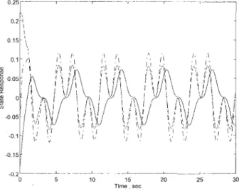
observing the growing trend of the system state when applying the feedback linearization control in Isidori, 1989. The reference trajectory is given by y„0) = 0.1 sin' (t). The input data functions are chosen to be M/(r) = cos ((i - l)wf). ci; = TT/ 10, (' = 1, 2, . . . , A^. Figure 2, in which the dash line indicates the reference trajectory and the solid line the system output, shows the finite-time tracking performance (T = 10) when only 5 input data functions (N = 5) are used in the control. If A^ is increased from 5 to 20, it is seen from Fig. 3 that the tracking performance is substantially improved, and this agrees with

114 / Vol. 120, MARCH 1998

Fig. 3 Tracking performance with 20 input data functions (A/ =^ 20)

Theorem 2 that the magnitude of the tracking error can be controlled by the number N. Figure 4 shows the infinite-time tracking result for the same reference trajectory, where T = 10 and N = 20 are used in the control (14). Figure 5 shows the system state, which confirms Theorem 3 that the system state

Fig. 4 Tracking performance of tlie infinite-time tracking control

f \ \ ' / i (^

15 Time , SGC

Fig. 5 State trajectories under the infinite-time tracl<ing control

A P P E N D I X A

Equation (10) can be easily proved by differentiation of the cost function (9) with respect to ©. One needs only to show that P(i(sO) is invertible due to the linear independence of the output data responses y°(t), ylit), . .., y%it). From the defi-nition of Po = <Fo, ^o), where Yo(t) = [y°,(t), yUt), . . . , yiit)], given any constant vector x G /?", one has x^PgX = /u u]{T)\\Yo(T)x\\^dT > 0, and hence X^PQX = 0 if and only if YO(T)X = 0 for all r E [0, T]. Since {y°{t), i = 1, 2, . . . , A'} are linearly independent on [0, T], Ygx = 0 only if ;c = 0. Therefore, it is concluded that X^PQX = 0 if and only if x = 0, and hence Po must be strictly positive definite.

Finally, direct substitution of 0 * into e{t) and J(&) shows that the minimal tracking error is as shown in Eq. (11), and the minimal cost is given by

7;$ = F,„o- VoPoVJ (Al)

= {y,no, y,no) - {y,„o, YO){YO, Yo)-'{y,„o, YoY'. (A2)

remains uniformly bounded under the proposed control. How-ever, the control input u(t) has small discontinuities at t = kT, k = 1, 2 , . . . , a problem that remains to be solved in the future.

7 Conclusions

A tracking control design for a class of LTV systems is introduced based on the assumption that a finite-time preview of the system matrices and the reference trajectory is available. The proposed design is based on a parameter optimization ap-proach, which minimizes the La-norm of the output tracking error. It is shown that as long as the preview time is longer than a critical value, the closed-loop system remains stable.

Acknowledgment

This research was supported by the National Science Council in Republic of China under Contract No. NSC 81-0401-E-002-554.

References

Arvanitis, K. G., and Paraskevopoulos, P. N., 1992, "Uniform Exact Model Matching for a Class of Linear Time-Varying Analytic Systems," Systems and

Control Letters, Vol. 19, pp. 313-323.

Benedetto, M. D., and Lucibello, P., 1993, "Inversion of Nonlinear Time-Varying Systems," IEEE Trans. Automat. Contr., Vol. 38, pp. 1259-1264.

Choura, S., 1992, "On the Design of Finite Time Setding Control for Linear

Systems," ASME JOURNAI, OP DYNAMIC SYSTEMS, MEASUREMENT, AND CONTROL,

Vol. 114, pp. 359-368.

Devasia, S., and Paden, B., 1994, "Exact Output Tracking for Nonlinear Time-Varying Systems," Proceedings of Conference on DecLuon cmd Control, pp. 2346-2354.

Gross, E., Tomizuka, M., and Messner, W., 1994, "Cancellation of Discrete Time Unstable Zeros by Feedforward Control," ASME JOURNAL OF DYNAMIC

SYSTEMS, MEASUREMENT, AND CONTROL, Vol. 116, pp. 3 3 - 3 8 .

Haack, B., and Tomizuka, M., 1991, "The Effect of Adding Zeros to

Feedfor-ward Controllers," ASME JOURNAL OF DYNAMIC SYSTEMS, MEASUREMENT, AND CONTROL, Vol. 113, pp. 6 - 1 0 .

Isidori, A., 1989, Nonlinear Control Systems, Springer-Verlag, Berlin. Kamen, E. W., 1989, "Tracking in Linear Time-Varying Systems,"

Proceed-ings of Conference on Decision and Control, pp. 263-268.

Kleinman, D., and Athans, M., 1968, "The Design of Suboptimal Linear Time-Varying Systems," IEEE Trans. Automat. Contr., Vol. 13, pp. 150-159.

Menq, C. H., and Xia, Z., 1990, "Characterization and Compensation of Dis-crete Time Nonminimum Phase Zeros for Precision Tracking Control," ASME

JOURNAL OP DYNAMIC SYSTEMS, MEASUREMENT, AND CONTROL, pp. 15-23.

Rudin, W., 1974, Real and Complex Analysis, McGraw-Hill, New York, NY. Tomizuka, M., 1987, "Zero Phase Error Tracking Algorithm for Digital

Con-trol," ASME JOURNAL OF DYNAMIC SYSTEMS, MEASUREMENT, AND CONTROL,

Vol. 109, pp. 65-68.

Tsakalis, K. S., and loannou, P. A., 1993, Linear Time-Varying Plants: Control

and Adaptation, Prentice-Hall, Englewood Cliffs, NJ.

Zhao, H., and Chen, D., 1994, "Minimum-Energy Approach to Stable hwersion of Nonminimum Phase Systems," Proceedings of the American Control

Confer-ence, pp. 2705-2709.

A P P E N D I X B

When there are W -I- 1 data pairs [M,(0> ^ . ( O ] available, the minimal cost function achieved is given by, according to Eq. ( A l ) , •^jv+i — Y,„a — VQP where P = ( B l ) p p(/V+ 1)X(W+I)

rPo' + Po'.vA"'i^Po'

A-'

in which Vo and PQ are as in Eq. ( A l ) , and

V = {yN+\, ymo) e P ' , w = {yN+i, yN+i) e p ' ,

^ = <3'o,y«+,>eP"

with Fo = [}'?. y", • • • . yw] • Using the formula for block matrix inverse, the second term in J'ti+i can be expressed as

%P-'Vl=[Va D]

V

= VoPo'Vl + is'''Po% - vVA-'{.s-^Po'vo ~ V) (B2) where A = (yN+uyN+t) - s^Po's G R*^ (it is shown in Appen-dix C that A is a positive number and hence invertible). Since

s^Pa'Vo - V = .9^0^; - i; = (3;^,+ ,, Fo)©« - (y^+i, }'„,o>

= (yw+i. Yo&* - y,„o) = -(yw+i, e*),

where Eq. (10) is used to obtain the first equality, and Eq. (11) the last equality, subtracting Eq. ( A l ) from Eq. ( B l ) results in

Jt+\ - J'N = -{yN+i, e*yA~'{yN+i, e*).

It then follows from the Hypothesis in (12) and the positiveness of A that 7w+i - J* < 0.

To prove Eq. (13),note that if the sequence >>;(?) is complete, the set of all finite linear combinations of ^ , ( 0 is dense in the L^ space on [0, T] (Theorem 4.18, Rudin, 1974). By quoting the Approximation Problem in Section 4.15 and Theorem 4.16 in Rudin (1974) it is concluded that given any desired g > 0, there exists a number A^ such that J^ < £• This concludes the proof for Eq. (13).

A P P E N D I X C

It will be shown that the number

A = (y^^u y^^i) - {y^^u Y){Y, F)-'<)'NH-,, YV ( C I ) in Eq. (B2) is a positive number if {yi, yz, . . . , yf/+i} are linear independent time functions. First, to show that A is non-negative, notice that A in Eq. ( C I ) has exactly the same form as J* in Eq. (A2) with y^+i in A acting as y^o in J*. Thus, A can be treated as the minimal cost function J* with a reference trajectory y„ given by

ymo = 9m - i^oixo) = yN+u Or y„= y^+i +Lo(Xo). Hence, A must be non-negative. Second, a contradiction argu-ment will be used to show that A is nonzero. Assuming that A = 0, it follows from the previous statement that

A = 7^

= 0 = I

iUt) - y*it)rdt

^^,+1(0 = -Lo(xo) + y*(t) = -Lo(xo) -I- Lo(xo) + L ( M * ) N

= UlO*u,) = I,9*yi{t) V f G [ 0 , n . However, the last equation is a contradiction with the fact that {y\,y2, • • •, yN+\} are Unearly independent. It is thus concluded that A =>= 0.

A P P E N D I X D

Discretize the closed-loop system (1) and (14) with a sam-pling period T to obtain

x[ik+ l)T]=Aik)x{kT) + D(k), fe = 0 , 1 , 2 , . . . ( D l ) where D(k) Jk ik+\)T m k + 1)T,T]B(T)U(T)P;' C(k+1)T X Jk! u!is)Ylis)y„is)dsdT, A{k) = Q,(k, T) - Q,(k, T)Pl\T)Q^(k, T), (D2) Mk+t)T Q,(k, T) = <^[{k + l)T, T]B(T)U(T)dT e if"^'" JkT Q2(k, T) = uj{s)Yl{s)C{s)^{.s, kT)ds G 7?"^" JkT Q3(k,T) = $[(fe+ l)T,kT].

Since the open-loop system (1) is exponentially stable, and the input data Uit) and the output data Y^(t) are all uniformly bounded, one can show that for all integer k and any time interval length T,

\\Q,(k,T)\\^Mu \\Q2{k, T)\\ s M2,

WQ^ik, T)\\ ^ me-^\ (D3) for some positive constants Mi and M2, and m and a are as in

Eq. ( 2 ) . Taking the matrix norm of A(fe) in Eq. (D2) and using Eq. (D3) result in

\\A{k)\\ ^ me-'^ + M,M:\\Pl\T) (D4)

The Remark before Theorem 3 shows that \\P~% is a strictly decreasing function of T. Hence, according to Eq. (D4), there exists a Tnin such that

||A(jfe)|| < 1, V/t > 0 and V r a T^ (D5) Finally, uniform boundedness oi x{kT) can be concluded by invoking the contraction mapping Theorem to Eq. ( D l ) , and by noting that 5 in Eq. ( D l ) is uniformly bounded since it is assumed that the input data U{t) and hence the output data Yi{t) are uniformly bounded.