鑑別式訓練法於語者驗證之研究

國

立

交

通

大

學

資訊科學與工程研究所

博

士

論

文

鑑別式訓練法於語者驗證之研究

Discriminative Training Methods for Speaker Verification

研 究 生：趙怡翔

指導教授：王新民 教授

張瑞川 教授

鑑別式訓練法於語者驗證之研究

Discriminative Training Methods for Speaker Verification

研 究 生：趙怡翔 Student：Yi-Hsiang Chao

指導教授：王新民 博士 Advisor：Dr. Hsin-Min Wang

張瑞川 博士

Dr. Ruei-Chuan Chang

國 立 交 通 大 學

資 訊 科 學 與 工 程 研 究 所

博 士 論 文

A Dissertation

Submitted to Department of Computer Science College of Computer Science

National Chiao Tung University in partial Fulfillment of the Requirements

for the Degree of Doctor of Philosophy

in

Computer Science

January 2009

Hsinchu, Taiwan, Republic of China

鑑別式訓練法於語者驗證之研究

學生：趙怡翔

指導教授

：

王新民 博士

張瑞川 博士

國立交通大學資訊科學與工程研究所

摘

要

語者驗證(speaker verification)常被表示成統計上的假說測定(hypothesis testing)問題，用似然 比例 (likelihood ratio, LR)檢定的方法來解。一個語者驗證系統性能的好壞高度依賴於目標語 者聲音的模型化(空假說)與非目標語者聲音的描述(替代假說)。然而，替代假說因為包含未知 的冒充者，通常很難被事先描述地好。在這篇論文，我們提出一個描述替代假說的較佳架構， 其目標是希望將目標語者與冒充者做最佳化的鑑別。該架構是建構在一群事先訓練好的背景語 者 的 可 用 資 訊 的 加 權 算 術 組 合 (weighted arithmetic combination, WAC) 或 加 權 幾 何 組 合 (weighted geometric combination, WGC)上。我們提出使用二種鑑別式訓練法來最佳化 WAC 或

WGC 的相關參數，分別是最小驗證誤差(minimum verification error, MVE)訓練法與演化式最小

驗證誤差(evolutionary minimum verification error, EMVE)訓練法，希望使得錯誤接受(false acceptance)機率與錯誤拒絕(false rejection)機率都能最小。此外，我們也提出二種基於 WAC 與

WGC 的 新 的 決 策 函 數 (decision functions) ， 其 可 以 被 視 為 非 線 性 鑑 別 分 類 器 (nonlinear

discriminant classifiers)。為了求解加權向量 w，我們提出使用二種基於核心的鑑別技術

(kernel-based discriminant techniques)，分別是基於核心的費氏鑑別器(Kernel Fisher Discriminant,

KFD)與支持向量機器(Support Vector Machine, SVM)，因為它們擁有能將目標語者與非目標語

在內文不相依(text-independent)語者驗證技術中，GMM-UBM 系統是最常被使用的主流方 法。其優點是目標語者模型與通用背景模型(universal background model, UBM) 都具有概括性 (generalization)的能力。然而，因為這二種模型是分別根據不同的訓練準則所求出，訓練過程

皆沒有考慮到目標語者模型與 UBM 之間的鑑別性(discriminability)。為了改進 GMM-UBM 方 法，我們提出一個鑑別式反饋調適(discriminative feedback adaptation, DFA)架構，希望可以同 時兼顧概括性與鑑別性。此架構不但保留了原本 GMM-UBM 方法的概括性能力，而且再強化 了目標語者模型與 UBM 之間的鑑別性能力。在 DFA 架構下，我們不是使用一個統一的通用 背景模型，而是建構一個具鑑別性的特定目標語者反模型(anti-model)。 在我們的實驗中，我們共使用 XM2VTSDB、ISCSLP2006-SRE 與 NIST2001-SRE 這三套語 者驗證資料庫(database)，實驗結果顯示我們所提出的方法優於所有傳統上基於 LR 的語者驗證 技術。

Discriminative Training Methods for Speaker Verification

Student：Yi-Hsiang Chao

Advisors：Dr. Hsin-Min Wang

Dr. Ruei-Chuan Chang

Department of Computer Science

National Chiao Tung University

ABSTRACT

Speaker verification is usually formulated as a statistical hypothesis testing problem and solved

by a likelihood ratio (LR) test. A speaker verification system’s performance is highly dependent on

modeling the target speaker’s voice (the null hypothesis) and characterizing non-target speakers’

voices (the alternative hypothesis). However, since the alternative hypothesis involves unknown

impostors, it is usually difficult to characterize a priori. In this dissertation, we propose a framework

to better characterize the alternative hypothesis with the goal of optimally distinguishing the target

speaker from impostors. The proposed framework is built on a weighted arithmetic combination

(WAC) or a weighted geometric combination (WGC) of useful information extracted from a set of

pre-trained background models. The parameters associated with WAC or WGC are then optimized

using two discriminative training methods, namely the minimum verification error (MVE) training

method and the proposed evolutionary MVE (EMVE) training method, such that both the false

acceptance probability and the false rejection probability are minimized. Moreover, we also propose

two new decision functions based on WGC and WAC, which can be regarded as nonlinear

discriminant techniques, namely the Kernel Fisher Discriminant (KFD) and Support Vector Machine

(SVM), because of their ability to separate samples of target speakers from those of non-target

speakers efficiently.

In recent years, the GMM-UBM system is the predominant approach for the text-independent

speaker verification task. The advantage of the approach is that both the target speaker model and

the impostor model (UBM) have generalization ability. However, since both models are trained

according to separate criteria, the optimization procedure can not distinguish a target speaker from

background speakers optimally. To improve the GMM-UBM approach, we propose a discriminative

feedback adaptation (DFA) framework that allows generalization and discrimination to be

considered jointly. The framework not only preserves the generalization ability of the GMM-UBM

approach, but also reinforces the discriminability between the target speaker model and the UBM.

Under DFA, rather than use a unified UBM, we construct a discriminative anti-model exclusively for

each target speaker.

The results of speaker-verification experiments conducted on three speech corpora, the Extended

M2VTS Database (XM2VTSDB), the ISCSLP2006-SRE database and the NIST2001-SRE database,

ACKNOWLEDGEMENTS

First, I am grateful to my advisor, Dr. Hsin-Min Wang, for his intensive suggestions, patient

guidance, and enthusiasm of research. Second, I am grateful to my another advisor, Dr. Ruei-Chuan

Chang, for his kindly helping and encouragement in my research. Third, I am grateful to Dr. Wei-Ho

Tsai for his helpful suggestions and assistance on my work. Thanks are also given to all members of

the Spoken Language Group, Chinese Information Processing Laboratory at IIS, Academia Sinica,

for their discussions. Finally, I would like to express my appreciation to my family for their

CONTENTS

ABSTRACT (IN CHINESE)……….……….…………

i

ABSTRACT (IN ENGLISH)………

iii

ACKNOWLEDGEMENTS………..

v

CONTENTS……….….

vi

LIST OF FIGURES………...…… viii

LIST OF TABLES………

ix

1 Introduction………...

1

1.1 Background………...……….…..

5

1.2 The Approaches of This Dissertation…...……….…..

10

1.3 The Organization of This Dissertation……….………..….

12

2 Improving the Characterization of the Alternative Hypothesis via Minimum

Verification Error Training………..…… 13

2.1 Characterization of the Alternative Hypothesis………...………… 15

2.2 Gradient-based Minimum Verification Error Training……….…………..

19

2.3 Evolutionary Minimum Verification Error Training………...……… 23

2.4 Experiments and Analysis………...………

26

3 Improving the Characterization of the Alternative Hypothesis Using Kernel

Discriminant Analysis……….……….……...……....

40

3.1 The Proposed Decision Functions………...

42

3.3 Concepts Related to the Characteristic Vector……… 47

3.4 Experiments and Analysis………...………

49

4 Improving GMM-UBM Speaker Verification Using Discriminative Feedback

Adaptation…….………..……

60

4.1 Discriminative Feedback Adaptation………... 62

4.2 Linear Regression-based MVSE (LR-MVSE) Adaptation……….

66

4.3 Eigenspace-based MVSE (E-MVSE) Adaptation……….…..

69

4.4 Simplified Versions of LR-MVSE and E-MVSE……… 74

4.5 Experiments and Analysis………...………

75

5 CONCLUSIONS ……….………..………. 82

LIST OF FIGURES

Fig. 1.1. Speaker recognition systems….………..……….

6

Fig. 2.1. The general scheme of a GA….………..……….

23

Fig. 2.2.

The learning curves of gradient-based MVE and EMVE for the

“Evaluation” subset in Configuration II………...

30

Fig. 2.3. DET curves for the “Test” subset in Configuration II………..

33

Fig. 2.4. Hybrid anti-model systems versus all baselines: DET curves for the

“Test” subset in Configuration II……….…

33

Fig. 2.5. DET curves for the “Test” subset in the NIST SRE-like configuration...

38

Fig. 3.1. Geometric Mean versus WGC: DET curves for the “Test” subset in

XM2VTSDB……….…... 51

Fig. 3.2. Arithmetic Mean versus WAC: DET curves for the “Test” subset in

XM2VTSDB... ………... 53

Fig. 3.3. Baseline systems versus WAC and WGC: DET curves for the

ISCSLP2006-SRE “Evaluation Data Set”.……….…….

59

Fig. 4.1. The proposed discriminative feedback adaptation framework…………

63

Fig. 4.2. The s function compared to the sigmoid function………....

65

Fig. 4.3. The minimum DCFs versus the number (J×B) of 3-second negative

training samples per target speaker………..

78

Fig. 4.4. Experiment results in DET curves. The circles indicate the minimum

DCFs……….…

79

Fig. 4.5. The DET curves of the LR-MVSE and E-MVSE systems and their

simplified versions. The circles indicate the minimum DCFs…...

81

LIST OF TABLES

Table 2.1. Configuration II of XM2VTSDB………..

27

Table 2.2. A summary of the parametric models used in each system…………..

28

Table 2.3. DCFs for the “Evaluation” and “Test” subsets in Configuration II…..

34

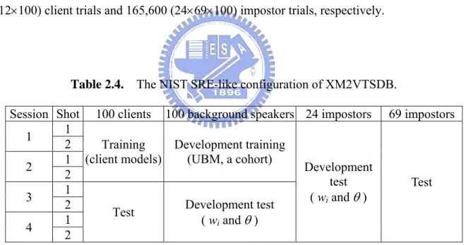
Table 2.4. The NIST SRE-like configuration of XM2VTSDB………....….

36

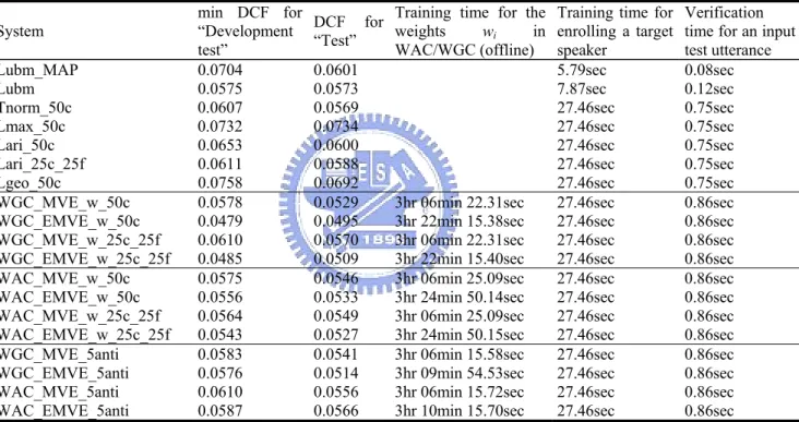
Table 2.5. DCFs for the “Development test” and “Test” subsets, together with

the running time evaluation in the NIST SRE-like configuration…....

39

Table 3.1. DCFs for the “Evaluation” and “Test” subsets in the XM2VTS

database……….

54

Table 3.2. Comparison of errors made by “WGC_RBF_KFD_w_20c” and

“Ari_10c_10f” ...

55

Table 3.3. Minimum DCFs and actual DCFs for the ISCSLP2006-SRE………..

58

Table 3.4. Comparison of errors made by “WGC_RBF_KFD_w_20c” and

“ Tnorm_50c”……….…………...

58

Chapter 1

Introduction

In many practical pattern recognition applications, it is necessary to make a binary decision, such as “yes/no” or “accept/reject”, with respect to an uncertain hypothesis that can only be validated through its observable consequences. In a statistical framework, the problem is generally formulated as a test that involves a null hypothesis, H0, and an alternative

hypothesis, H1, regarding some decision function L(⋅) for a given observation X:

, ) ( : ) ( : 1 0 θ θ < ≥ X L H X L H (1.1)

where θ is the decision threshold. Depending on the application, various decision functions can be designed. The most popular decision function computes the ratio of possibilities between the null hypothesis and the alternative hypothesis as follows:

⎩ ⎨ ⎧ < ≥ = , ) reject i.e., ( accept accept ) ( ) ( ) ( 0 1 0 1 0 H H H X L X L X L H H θ θ (1.2)

where denotes a certain possibility measure of X with respect to the hypothesis Hi. For example, could be the likelihood probability that

hypothesis Hi gives X, and the resulting L(⋅) represents a so-called likelihood ratio (LR)

function. If we represent the observation X as a sequence of r–dimensional feature vectors and assume that the feature vector sequence of X is independent and identically

0,1, ), (X i= L i H } o ) (X L i H p(X |Hi) , , {o _K

distributed (i.i.d.), the likelihood of the observation X given the hypothesis Hi, i = 0 or 1, can be computed by ). | ( ) | ( 1 t i T t i p o H H X p = ∏ = (1.3) In the implementation, H0 and H1 can be characterized by some parametric models, which are

usually denoted as λ (the null hypothesis model or target model) and λ (the alternative hypothesis model or anti-model). Suppose both λ and λ are characterized by Gaussian mixture models (GMMs) [Reynolds 1995, 2000], the probability density functions (pdf) of each feature vector ot given H0 and H1 can be respectively defined as

∑

= = = 0 1 0 0 0) ( |λ) ( | ) | ( M m m t m t t H p o p p o o p g (1.4) and , ) | ( ) λ | ( ) | ( 1 1 1 1 1

∑

= = = M m m t m t t H p o p p o o p g (1.5) where , i = 0 or 1, , is the mixture weight that satisfies the constraint

; is the m-th Gaussian mixture component of the target model λ (i = 0) or the alternative hypothesis model

i m p = i m p i M m=1,..., ) i m Σ 1 1

∑

= i M m ~ ( , i m i m N μ g

λ (i = 1) with the r×1 mean vector and the

r×r covariance matrix ; and is the Gaussian density function that is expressed

as i m μ i m Σ i ) m g | (ot p . ) ( ) ( )' ( 2 1 exp | | ) 2 ( 1 ) | ( 1 2 / 1 2 / _⎭⎬ ⎫ ⎩ ⎨ ⎧_{− − −} = − i m t i m i m t i m r i m t o o o p μ Σ μ Σ g π (1.6)

However, in most real applications, the alternative hypothesis model λ is usually ill-defined and difficult to characterize a priori. For example, in speaker verification [Bimbot

2004; Faundez-Zanuy 2005; Fauve 2007; Przybocki 2007; Van Leeuwen 2006], the problem of determining if a speaker is who he or she claims to be is normally formulated as follows: given an unknown utterance U, determine whether

H0: U is from the target speaker, or

H1: U is not from the target speaker.

Though H0 can be modeled straightforwardly using speech utterances from the target speaker,

H1 does not involve any specific speaker, and hence lacks explicit data for modeling. As a

result, various approaches have placed special emphasis on better characterization of H1. One

popular approach pools all the speech data from a large number of background speakers and trains a single speaker-independent GMM Ω, called the world model or the universal background model (UBM) [Reynolds 2000]. During a test, the logarithmic LR measure that an unknown utterance U was spoken by the claimed speaker can be evaluated by

), | ( log ) λ | ( log ) ( UBM U = pU − p U L Ω (1.7)

where λ is the target speaker GMM trained using speech from the claimed speaker. The larger the value of LUBM(U), the more likely it is that the utterance U was spoken by the claimed

speaker. Due to the good generalization ability of the UBM, LUBM(U) (usually called the

GMM-UBM method [Reynolds 2000] is considered as a current state-of-the-art solution to the text-independent speaker verification problem.

Instead of using a single model, an alternative approach is to train a set of GMMs {λ1,

λ2,…, λB} using speech from several representative speakers, called a cohort [Rosenberg 1992],

which simulates potential impostors. This leads to the following possible logarithmic LR measures, where the alternative hypothesis can be characterized by:

(i) the likelihood of the most competitive cohort model [Liu 1996], i.e., ), λ | ( log max ) λ | ( log ) ( Max U p U pU i L = − (1.8)

(ii) the arithmetic mean of the likelihoods of the B cohort models [Reynolds 1995], i.e., , ) λ | ( log ) λ | ( log ) ( 1 Ari ⎭ ⎬ ⎩ ⎨ − =

∑

= i i U p B U p U L ⎧1 ⎫ B (1.9)

(iii) the geometric mean of the likelihoods of the B cohort models [Liu 1996], i.e., .) λ | ( log 1 ) λ | ( log ) ( 1 Geo

∑

= − = B i i U p B U p U L (1.10)

In a well-known score normalization method called T-norm [Auckenthaler 2000; Sturim 2005], LGeo(U) is divided by the standard deviation of the log-likelihoods of the B cohort

models.

The LR measures in Eqs. (1.7) – (1.10) can be collectively expressed in the following general form [Reynolds 2000]:

(

( |λ ), ( |λ ),..., ( |λ )

)

, ) λ | ( ) ( 2 1 p U pU N U p U p U L Ψ = (1.11)

where Ψ(⋅) denotes a certain function of the likelihoods computed for a set of so-called background models {λ1, λ2,…, λN}. For example, if the background model set is generated

from a cohort, letting Ψ(⋅) be the maximum function gives LMax(U), while the arithmetic mean

gives LAri(U), and the geometric mean gives LGeo(U). When Ψ(⋅) is an identity function, N = 1,

and λ1 = Ω, Eq. (1.11) becomes LUBM(U).

However, there is no theoretical evidence to indicate which method of characterizing H1

is optimal, and the selection of Ψ(⋅) is usually application and training data dependent. More specifically, a simple function, such as the arithmetic mean, the maximum, or the geometric mean, is a heuristic that does not involve any optimization process. Thus, the resulting system is far from optimal in terms of verification accuracy. Although the GMM-UBM method is a current state-of-the-art solution to the text-independent speaker verification problem, there is

no optimization process of characterizing H1 to support its discriminability.

Before the presentation of the proposed frameworks for speaker verification problems, we introduce some backgrounds about the current GMM-based speaker recognition methods.

1.1. Background

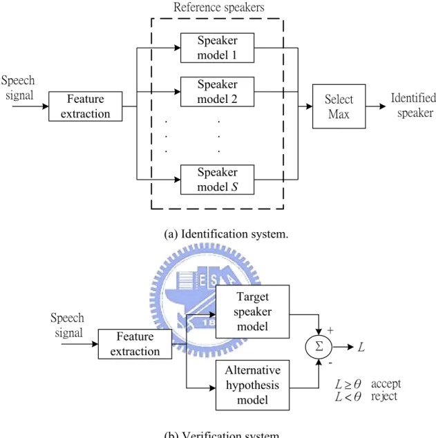
Over the past several years, GMM has become the dominant modeling approach in speaker recognition applications. Speaker recognition can be classified into identification and verification. In speaker identification, the system has trained models for a certain amount of speakers and the task is to determine which one of these models best matches the current speaker. In verification, the identity of the current speaker is somehow transmitted to the system beforehand and the task is to determine whether the current speaker is the claimed one or not. Speaker recognition methods can also be divided into text-dependent and text-independent methods. The former requires the speaker to say keywords or sentences having the same text for both training and recognition trials, while the latter does not rely on a specific text being spoken.

Fig. 1.1 shows the block diagrams of the speaker identification and verification systems. The process of feature extraction is to transform the speech signal into a set of feature vectors, and the goal is to obtain a new representation which is more compact, less redundant, and more suitable for statistical modeling and the calculation of a distance or any other kind of score. In recent years, Mel-scale frequency cepstral coefficient (MFCC) [Huang 2001] is the most popular feature vector used in speech and speaker recognition systems. The mel-scale cepstrum is the discrete cosine transform (DCT) of the log-spectral energies of the speech segment. The spectral energies are calculated over logarithmically spaced filters with increasing bandwidths (mel-filters). MFCC-based GMMs [Reynolds 1995] have been

successfully applied to speaker recognition systems recently. In the following, we introduce two commonly-used statistical modeling methods for estimating the parameters of GMMs.

Feature extraction Speaker model 1 Speaker model 2 Speaker model S

(a) Identification system.

Feature extraction Target speaker model Alternative hypothesis model Speech signal Σ + -θ <θ ≥ accept reject (b) Verification system.

Fig. 1.1. Speaker recognition systems.

1.1.1. Maximum Likelihood (ML) Estimation Technique

Given the training speech data from a speaker, U={o₁,K ,oT}, the goal of maximum

likelihood (ML) estimation is to find the parameters of the GMM, λ, which maximize the likelihood of the GMM:

). λ | ( ) λ | ( 1 t T t o p U p = ∏ = (1.12) Eq. (1.12) is a nonlinear function of the GMM parameters and direct maximization is infeasible. However, the ML parameter estimation can be achieved iteratively via the expectation-maximization (EM) algorithm [Huang 2001].

The basic idea of the EM algorithm is, beginning with an initial model λ, to estimate a new model λˆ , such that . The new model then becomes the initial model for the next iteration and the process is repeated until some convergence condition is reached. This is the same basic technique used for estimating hidden Markov model (HMM) parameters via the Baum-Welch re-estimation algorithm [Huang 2001].

) λ | ( ) λˆ | (U pU p ≥

In each EM iteration, the following re-estimation formulae, which guarantee a monotonic increase in the model’s likelihood value, are used:

Mixture Weights: .) λ , | ( 1 ˆ 1

∑

= = T t t m p m o T p (1.13) Mean vectors: . ) λ , | ( ) λ , | ( ˆ 1 1

∑

∑

= = = _T t t T t t t m o m p o o m p μ (1.14) Covariance matrices: . ) λ , | ( ) ˆ )( ˆ )( λ , | ( ˆ 1 1

∑

∑

= = − − ′ = _T t t T t t t m t m m o m p o o o m p μ μ Σ (1.15)

We usually assume that all covariance matrices of the GMM, m = 1,…, M, are diagonal, and the variance vector . The a posteriori probability for the m-th Gaussian

m Σ ) ( diag 2 m m Σ σ =

mixture component g_m is given by , ) | ( ) | ( ) λ , | ( 1

∑

= = _M i i t i m t m t o p p o p p o m p g g (1.16)

where is the original mixture weight and is the Gaussian density function defined in Eq. (1.6).

m

p p(o_t |g_m)

Selecting the order M of the mixture and initializing the model parameters prior to the EM algorithm are two critical factors in training a GMM. There are no good theoretical means to guide one in either of these selections, so they are best experimentally determined for a given task.

1.1.2. Maximum A Posteriori (MAP) Estimation Technique

Conventional GMMs trained from the EM algorithm perform well only when a large amount of training data is available to characterize the characteristics of the speaker. For each speaker, this approach needs a large amount of training data to train a GMM so as to cover all the possible pronunciations of this speaker, in particular when the speaker recognition is conducted under the text-independent mode. Due to this characteristic, the performance of GMM deteriorates drastically when the training data are sparse. However, client speakers definitely prefer to enroll with as little speech as possible. To solve this problem, speaker adaptation approaches have been investigated in recent years.

One successful adaptation approach, namely the UBM-MAP approach, has been widely used in text-independent speaker verification tasks. This approach first pools all speech data from a large number of background speakers to train a universal background model (UBM) via the EM algorithm. Unlike the standard approach of maximum likelihood training of the speaker model independently of the UBM, this approach then adapts the well-trained UBM to

a speaker model λ using this speaker’s training speech via the maximum a posteriori (MAP) estimation technique. The adapted GMM λ is effective because its generalization ability allows λ to handle acoustic patterns not covered by the limited training data of the speaker.

The specifics of the adaptation are as follows. Given a UBM, Ω, and training vectors from the target speaker, , we first computer the a posteriori probability

for the m-th Gaussian mixture component , m = 1,…, M, of the UBM: } , , {o₁ o_T U= _K ) , | (m o_t Ω p g_m , ) | ( ) | ( ) , | ( 1

∑

= = Ω _M i i t i m t m t o p p o p p o m p g g (1.17)

Then, we use and ot to compute the sufficient statistics for the mixture weight,

mean, and variance parameters: ) , | (m o_t Ω p ‡ , ) , | ( 1

∑

= Ω = T t t m p m o n (1.18) , ) , | ( 1 ) ( 1

∑

= Ω = T t t t m m p m o o n o E (1.19) . ) , | ( 1 ) ( 1 2 2

∑

= Ω = T t t t m m p m o o n o E (1.20) This is the same as the expectation step in the EM algorithm.

Finally, these new sufficient statistics from the training data are used to update the old UBM sufficient statistics from the m-th mixture to create the adapted parameters for the m-th mixture with the equations:

, ] ) 1 ( / [ ˆ n T p c p_m = ε_{m m} + −ε_{m m} (1.21) ‡ _x2 _{is shorthand for diag (xx’).}

, ) 1 ( ) ( ˆ_{m m}E_m o _m μ_m μ =ε + −ε (1.22) and , ˆ ) )( 1 ( ) ( ˆ2 2 2 2 2 m m m m m m m E o σ μ μ σ =ε + −ε + − (1.23) where the scale factor c is computed over all adapted mixture weights to ensure that they sum to 1 and the adaptation coefficients εm controlling the balance between old and new estimates

is defined as , r n n m m m = ₊ ε (1.24) where r is a fixed relevance factor. After adaptation, the mixture components of the adapted GMM retain a correspondence with the mixtures of the UBM.

1.2. The Approaches of This Dissertation

In speaker recognition tasks, as the ML or MAP estimation technique has become the standard modeling method for characterizing the target speaker (the null hypothesis), this dissertation focuses on two issues: the improvement of the characterization of the alternative hypothesis and the improvement of the current state-of-the-art GMM-UBM method.

1.2.1. Using Minimum Verification Error Training

To handle the speaker-verification problem more effectively, it is necessary to design a trainable mechanism for Ψ(⋅) defined in Eq. (1.11). We therefore propose a framework to better characterize the alternative hypothesis with the goal of optimally distinguishing the target speaker from impostors. The proposed framework is built on a weighted arithmetic

combination (WAC) or a weighted geometric combination (WGC) of useful information extracted from a set of pre-trained background models. The parameters associated with WAC or WGC are then optimized using two discriminative training methods, namely, the minimum verification error (MVE) training method [Chou 2003; Rosenberg 1998] and the proposed evolutionary MVE (EMVE) training method, such that both the false acceptance probability and the false rejection probability are minimized. The results of speaker verification experiments conducted on the Extended M2VTS Database (XM2VTSDB) [Messer 1999] demonstrate that the proposed frameworks along with the MVE or EMVE training outperform conventional LR-based approaches.

1.2.2. Using Kernel Discriminant Analysis

In contrast to the MVE training methods with the goal of minimizing both the false acceptance probability and the false rejection probability, we further propose two new decision functions based on WGC and WAC, which can be regarded as nonlinear discriminant classifiers. To obtain a reliable set of weights, the goal here is to separate the target speaker from imposters optimally. Thus, we apply kernel-based techniques, namely the Kernel Fisher Discriminant (KFD) [Mika 1999, 2002] and Support Vector Machine (SVM) [Burges 1998], to solve the weights, by virtue of their good discrimination ability. Our proposed approaches have two advantages over existing methods. The first is that they embed a trainable mechanism in the decision functions. The second is that they convert variable-length utterances into fixed-dimension characteristic vectors, which are easily processed by kernel discriminant analysis. The results of experiments conducted on both the XM2VTSDB and the ISCSLP2006-SRE database show that the proposed kernel-based decision functions outperform all of the conventional approaches.

1.2.3. Using Discriminative Feedback Adaptation

The GMM-UBM system [Reynolds 2000] is the predominant approach for text-independent speaker verification because both the target speaker model and the impostor model (UBM) have generalization ability to handle “unseen” acoustic patterns. However, since GMM-UBM uses a common anti-model, namely UBM, for all target speakers, it tends to be weak in rejecting impostors’ voices that are similar to the target speaker’s voice. To overcome this limitation, we propose a discriminative feedback adaptation (DFA) framework that reinforces the discriminability between the target speaker model and the anti-model, while preserving the generalization ability of the GMM-UBM approach. This is achieved by adapting the UBM to a target speaker dependent anti-model based on a minimum verification squared-error criterion, rather than estimating the model from scratch by applying the conventional discriminative training schemes. The results of experiments conducted on the NIST2001-SRE database show that DFA substantially improves the performance of the conventional GMM-UBM approach.

1.3. The Organization of This Dissertation

The remainder of this dissertation is organized as follows. Chapter 2 and 3 describe, respectively, the MVE training methods and the kernel discriminant analysis techniques used to improve the characterization of the alternative hypothesis. Chapter 4 introduces the proposed DFA framework for improving the GMM-UBM method. Then, in Chapter 5, we present our conclusions.

Chapter 2

Improving the Characterization of the

Alternative Hypothesis via Minimum

Verification Error Training

To handle the speaker-verification problem more effectively, we propose a framework that characterizes the alternative hypothesis by exploiting information available from background models, such that the utterances of the impostors can be more effectively distinguished from those of the target speaker. The framework is built on either a weighted geometric combination (WGC) or a weighted arithmetic combination (WAC) of the likelihoods computed for background models. In contrast to the geometric mean in LGeo(U) defined in Eq.

(1.6) or the arithmetic mean in LAri(U) defined in Eq. (1.5), both of which are independent of

the system training, our combination scheme treats the background models unequally according to how close each individual is to the target speaker model, and quantifies the unequal nature of the background models by a set of weights optimized in the training phase. The optimization is carried out with the minimum verification error (MVE) criterion [Chou 2003; Rosenberg 1998], which minimizes both the false acceptance probability and the false rejection probability. Since the characterization of the alternative hypothesis is closely related to the verification accuracy, the resulting system is expected to be more effective and robust than those of conventional methods.

The concept of MVE training stems from minimum classification error (MCE) training [Juang 1997; Siohan 1998; McDermott 2007; Ma 2003], where the former could be a special case of the latter when the classes to be distinguished are binary. Although MVE training has been extensively studied in the literature [Chou 2003; Rosenberg 1998; Sukkar 1996, 1998; Rahim 1997; Kuo 2003; Siu 2006], most studies focus on better estimating the parameters of the target model. In contrast, we try to improve the characterization of the alternative hypothesis by applying MVE training to optimize the parameters associated with the combinations of the likelihoods from a set of background models. Traditionally, MVE training has been realized by the gradient descent algorithms, e.g., the generalized probability descent (GPD) [Chou 2003], but the approach only guarantees to converge to a local optimum. To overcome such a limitation, we propose a new MVE training method, called evolutionary MVE (EMVE) training, for learning the parameters associated with WAC and WGC based on a genetic algorithm (GA) [Eiben 2003]. It has been shown in many applications that GA-based optimization is superior to gradient-based optimization, because of GA’s global scope and parallel searching power. To facilitate the EMVE training, we designed a new mutation operator, called the one-step gradient descent operator (GDO), for the genetic algorithm. The results of speaker verification experiments conducted on the Extended M2VTS Database (XM2VTSDB) [Messer 1999] demonstrate that the proposed methods outperform conventional LR-based approaches.

The remainder of this chapter is organized as follows. Section 2.1 presents the proposed methods for characterizing the alternative hypothesis. Sections 2.2 and 2.3 describe, respectively, the gradient-based MVE training and the EMVE training used to optimize our methods. Section 2.4 contains the experiment results.

2.1. Characterization of the Alternative Hypothesis

To characterize the alternative hypothesis, we generate a set of background models using data that does not belong to the target speaker. Instead of using the heuristic arithmetic mean or geometric mean, our goal is to design a function Ψ(⋅) that optimally exploits the information available from background models. In this section, we present our approach, which is based on either the weighted arithmetic combination (WAC) or the weighted geometric combination (WGC) of the useful information available. Moreover, the LR measure based on WAC or WGC can be viewed as a generalized and trainable version of LUBM(U) in Eq. (1.3), LMax(U)

in Eq. (1.4), LAri(U) in Eq. (1.5), or LGeo(U) in Eq. (1.6).

2.1.1. The Weighted Arithmetic Combination (WAC)

First, we define the function Ψ(⋅) in Eq. (1.7) based on the weighted arithmetic combination as , ) λ | ( )) λ | ( ),..., λ | ( ( ) λ | ( 1 1

∑

= = Ψ = N i i i N w pU U p U p U p (2.1)

where wi is the weight of the likelihood p(U | λi) subject to

∑

_iN₌₁wi =1. This function assigns

different weights to N background models to indicate their individual contribution to the alternative hypothesis. Suppose all the N background models are Gaussian Mixture Models (GMMs); then, Eq. (2.1) can be viewed as a mixture of Gaussian mixture density functions. From this perspective, the alternative hypothesis model λ can be viewed as a GMM with two layers of mixture weights, where one layer represents each background model and the other represents the combination of background models.

2.1.2. The Weighted Geometric Combination (WGC)

Alternatively, we can define the function Ψ(⋅) in Eq. (1.7) from the perspective of the weighted geometric combination as

. ) λ | ( )) λ | ( ),..., λ | ( ( ) λ | ( 1 1 i w i N i N pU U p U p U p = ∏ = Ψ = (2.2) Similar to the weighted arithmetic combination, Eq. (2.2) considers the individual contribution of a background model to the alternative hypothesis by assigning a weight to each likelihood value. One additional advantage of WGC is that it avoids the problem where

0 ) λ |

(U →

p . The problem can arise with the heuristic geometric mean because some values of the likelihood may be rather small when the background models λi are irrelevant to an

input utterance U, i.e., p(U| λi) → 0. However, if a weight is attached to each background

model, Ψ(⋅) defined in Eq. (2.2) should be less sensitive to a tiny value of the likelihood; hence, it should be more robust and reliable than the heuristic geometric mean.

2.1.3. Relation to Conventional LR Measures

We observe that Eq. (2.1) and Eq. (2.2) are equivalent to the arithmetic mean and the geometric mean, respectively, when wi = 1/N, i = 1,2,…, N; in other words, all the background

models are assumed to contribute equally. It is also clear that both Eq. (2.1) and Eq. (2.2) will degenerate to a maximum function if we set w_i* =1, where i*=argmax1≤i≤N p(U|λi), and

wi = 0, . Furthermore, the logarithmic LR measure based on Eq. (2.1) or Eq. (2.2)

will degenerate to LUBM(U) in Eq. (1.3) if only a UBM Ω is used as the background model.

Thus, both WAC- and WGC-based logarithmic LR measures can be viewed as generalized and trainable versions of LUBM(U) in Eq. (1.3), LMax(U) in Eq. (1.4), LAri(U) in Eq. (1.5), or

LGeo(U) in Eq. (1.6).

*

i i≠ ∀

In the WAC method, we refer to the alternative hypothesis model λ defined in Eq. (2.1) as a 2-layer GMM (GMM2), since it involves both inner and outer mixture weights. GMM2 differs from the UBM Ω in that it characterizes the relationship between individual background models through the outer mixture weights, rather than simply pooling all the available data and training a single background model represented by a GMM. Note that the inner and outer mixture weights are trained by different algorithms. Specifically, the inner mixture weights are estimated using the standard expectation-maximization (EM) algorithm [Huang 2001], while the outer mixture weights are estimated using minimum verification error (MVE) training or evolutionary MVE (EMVE) training, which we will discuss in Sec. 2.2 and Sec. 2.3, respectively. In other words, GMM2 integrates the Bayesian learning and discriminative training algorithms. The objective is to optimize the LR measure by considering the null hypothesis and the alternative hypothesis jointly.

2.1.4. Background Model Selection

In general, the more speakers that are used as background models, the better the characterization of the alternative hypothesis will be. However, it has been found [Reynolds 1995; Rosenberg 1992; Liu 1996; Higgins 1991; Auckenthaler 2000; Sturim 2005] that using a set of pre-selected representative models usually makes the system more effective and efficient than using the entire collection of available speakers. For this reason, we present two approaches for selecting background models to strengthen our WAC- and WGC-based methods.

A. Combining cohort models and the world model

Our first approach selects B+1 background models, comprised of B cohort models used in

and WGC in Eq. (2.2). Depending on the definition of a cohort, we consider two commonly-used methods [Reynolds 1995]. One selects the B closest speaker models {λcst 1,

λcst 2, …, λcst B} for each target speaker; and the other selects the B/2 closest speaker models

{λcst 1, λcst 2, …, λcst B/2}, plus the B/2 farthest speaker models {λfst 1, λfst 2, …, λfst B/2}, for each

target speaker. Here, the degree of closeness is measured in terms of the pairwise distance defined in [Reynolds 1995]: , ) λ | ( ) λ | ( log ) λ | ( ) λ | ( log ) λ , λ ( i j j j j i i i j i U p U p U p U p d = + (2.3) where λi and λj are speaker models trained using the i-th speaker’s utterances Ui and the j-th

speaker’s utterances Uj, respectively. As a result, each target speaker has a sequence of

background models, {Ω, λcst 1, λcst 2, …, λcst B} or {Ω, λcst 1, …, λcst B/2, λfst 1, …, λfst B/2}, for

Eqs. (1.7), (2.1), and (2.2).

B. Combining multiple types of anti-models

As shown in Eqs. (1.3) – (1.6), various types of anti-models have been studied for conventional LR measures. However, none of the LR measures developed thus far has proved to be absolutely superior to any other. Usually, LUBM(U) tends to be weak in rejecting

impostors with voices similar to the target speaker’s voice, while LMax(U) is prone to falsely

rejecting a target speaker; LAri(U) and LGeo(U) are between these two extremes. The

advantages and disadvantages of different LR measures motivate us to combine them into a unified LR measure because of the complementary information that each anti-model can contribute.

Consider K different LR measures Li(U), each with an anti-model λ , i = 1,2,…, K. If i

we treat each anti-model λ as a background model, the function Ψ(⋅) in Eq. (1.7) can be _i rewritten as,

(

( |λ ), ( |λ )..., ( |λ )

)

. ) λ | (U pU ₁ pU ₂ pU _K p =Ψ (2.4) Using WAC or WGC to realize Eq. (2.4), we can form a trainable version of the conventional LR measures in Eqs. (1.3) – (1.6), where each anti-model λ , i = 1,…,4, is computed, _i respectively, by ), | ( ) λ | (U ₁ = Up Ω p (2.5) ), λ | ( max ) λ | ( 1 2 _{i B} p U i U p ≤ ≤ = (2.6) , ) λ | ( 1 ) λ | ( 1 3

∑

= = B i i U p B U p (2.7) and . ) λ | ( ) λ | ( 1 1 4 B i B i pU U p ⎟ ⎠ ⎞ ⎜ ⎝ ⎛∏ = = (2.8)

As a result, for Eq. (1.7), each target speaker has the following sequence of background models, {λ₁,λ₂,λ₃,λ₄}. We denote systems that combine multiple anti-models as hybrid

anti-model systems.

2.2. Gradient-based Minimum Verification Error Training

After representing Ψ(⋅) as a trainable combination of likelihoods, the task becomes a matter of solving the associated weights. To obtain an optimal set of weights, we propose using minimum verification error (MVE) training [Chou 2003, Rosenberg 1998].

The concept of MVE training stems from MCE training, where the former could be a special case of the latter when the classes to be distinguished are binary. To be specific,

consider a set of class discriminant functions gi(U), i = 0,1,…, M - 1. The misclassification

measure in the MCE method [Juang 1997] is defined as

, ] ) ( exp[ 1 1 log ) ( ) ( / 1 , η i j j j i i g U M U g U d _⎥ ⎦ ⎤ ⎢ ⎣ ⎡ − + − =

∑

≠ η (2.9) where η is a positive number. If M = 2, η = 1, and

⎩ ⎨ ⎧ = = = , 1 if ) λ | ( log 0 if ) λ | ( log ) ( i U p i U p U g_i (2.10) then di(U) is reduced to the mis-verification measure defined in the MVE method:

⎩ ⎨ ⎧ ∈ = ∈ − = = , if ) ( ) ( if ) ( ) ( ) ( 1 1 0 0 H U U L U d H U U L U d U d (2.11)

where L(U) is the logarithmic LR. We further express L(U) as the following equivalent test

⎩ ⎨ ⎧ < ≥ − − = , accept 0 accept 0 ) λ | ( log ) λ | ( log ) ( 1 0 H H U p U p U L θ (2.12)

so that the decision threshold θ can also be included in the optimization process. Then, the mis-verification measure is converted into a value between 0 and 1 using a sigmoid function

)) ( exp( 1 1 )) ( ( U d U d sg ⋅ − + = ε , (2.13) where ε is a slope of the sigmoid function sg(⋅).

Next, we define the loss of each hypothesis as the average of the mis-verification measures of the training samples

, )) ( ( 1

_∑

∈ = i H U i i sg d U N l (2.14)

where l0 denotes the loss associated with false rejection errors, l1 denotes the loss associated

and impostors, respectively. Finally, we define the overall expected loss as (2.15) , 1 1 0 0l xl x D= +

where x0 and x1 indicate which type of error is of greater concern in a practical application.

Accordingly, our goal is to find the weights wi in Eq. (2.1) and Eq. (2.2) such that Eq.

(2.15) can be minimized. This can be achieved by using the gradient descent algorithm [Chou 2003]. To ensure that the weights satisfy

∑

N₌ =

i1wi 1, we solve wi by means of an

intermediate parameter αi, where

∑

= = _N j j i i w 1 ) exp( ) exp( α α , (2.16)

which is similar to the strategy used in [Juang 1997]. Parameter αi is iteratively optimized

using i t i t i D α δ α α ∂ ∂ − = +1) () ( _{, (2.17)}

where δ is the step size, and

[

]

[

1 ( ( ))

]

, )) ( ( 1 )) ( ( 1 )) ( ( 1 1 0 1 1 0 0 1 1 0 0 1 1 0 0

∑

∑

∈ ∈ ⎭ ⎬ ⎫ ⎩ ⎨ ⎧ ∂ ∂ ⋅ − ⋅ ⋅ + ⎪⎭ ⎪ ⎬ ⎫ ⎪⎩ ⎪ ⎨ ⎧ ⎟⎟ ⎠ ⎞ ⎜⎜ ⎝ ⎛ ∂ ∂ − ⋅ − − − ⋅ ⋅ = ∂ ∂ ⋅ ∂ ∂ ⋅ ∂ ∂ ⋅ ∂ ∂ + ∂ ∂ ⋅ ∂ ∂ ⋅ ∂ ∂ ⋅ ∂ ∂ = ∂ ∂ + ∂ ∂ = ∂ ∂ H U i H U i i i i i i L U L sg U L sg a N x L U L sg U L sg a N x L L d d sg sg x L L d d sg sg x x x D α α α α α α α l l l l (2.18) where . 1 1 ⎟ ⎟ ⎠ ⎞ ⎜ ⎜ ⎝ ⎛ ∂ ∂ − ∂ ∂ = ⎟ ⎟ ⎠ ⎞ ⎜ ⎜ ⎝ ⎛ ∂ ∂ ⋅ ∂ ∂ = ∂ ∂

∑

∑

= = j N j j i i N j i j j i w L w w L w w w L L α α (2.19)

If WAC is used, then . ) λ | ( ) λ | ( log_⎜⎜⎛

∑

_⎟⎟⎞= − ∂ ∂ − = ∂ ∂ N i N j j U p U p w w w L ) λ | ( 1 1

∑

= = ⎠ ⎝ j j j j i i _{w p U} (2.20) If WGC is used, then ). λ | ( log ) λ | ( log 1 i N j j j i i U p U p w w w L ₌₋ ⎟⎟ ⎠ ⎞ ⎜⎜ ⎝ ⎛ ∂ ∂ − = ∂ ∂

_∑

= (2.21)

The threshold θ in Eq. (2.12) can be estimated using , ) ( ) 1 ( θ δ θ θ ∂ ∂ − = + t D t _(2.22) where

[

1 ( ( ))

]

1 ( ( ))

[

1 ( ( ))

]

. )) ( ( 1 1 0 1 1 0 0 1 1 0 0

∑

∑

∈ ∈ − ⋅ ⋅ − − − − ⋅ ⋅ = ∂ ∂ ⋅ ∂ ∂ ⋅ ∂ ∂ ⋅ ∂ ∂ + ∂ ∂ ⋅ ∂ ∂ ⋅ ∂ ∂ ⋅ ∂ ∂ = ∂ ∂ H U H U U L sg U L sg a N x U L sg U L sg a N x L L d d sg sg x L L d d sg sg x D θ θ θ l l (2.23) In our implementation, the overall expected loss is set as

. ) 1

(

1

0 Target FalseAlarm Target Miss P C P

C

D= ×_l × + ×_l × − (2.24) Eq. (2.24) simulates the Detection Cost Function (DCF) [Van Leeuwen 2006]

), 1 ( _Target FalseAlarm FalseAlarm Target Miss Miss DET C P P C P P C = × × + × × − (2.25)

where CMiss denotes the cost of the miss (false rejection) error; CFalseAlarm denotes the cost of

the false alarm (false acceptance) error; PMiss ≈ l0 is the miss (false rejection) probability;

PFalseAlarm ≈ l1 is the false alarm (false acceptance) probability; and PTarget is the a priori

2.3. Evolutionary Minimum Verification Error Training

As the gradient descent approach may converge to an inferior local optimum, we propose an evolutionary MVE (EMVE) training method that uses a genetic algorithm (GA) to train the weights wi and the threshold θ in WAC- and WGC-based LR measures. It has been shown in

many applications that GA-based optimization is superior to gradient-based optimization, because of GA’s global scope and parallel searching power.

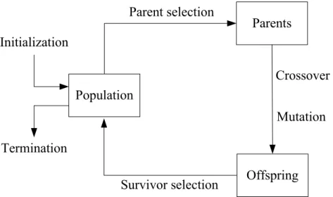
Genetic algorithms belong to a particular class of evolutionary algorithms inspired by the process of natural evolution [Eiben 2003]. As shown in Fig. 2.1, the operators involved in the evolutionary process are: encoding, parent selection, crossover, mutation, and survivor selection. GAs maintain a population of candidate solutions and perform parallel searches in the search space via the evolution of these candidate solutions.

To accommodate GA to EMVE training, the fitness function of GA is set as the reciprocal of the overall expected loss D defined in Eq. (2.15), where and . The details of the GA operations in EMVE training are described in the following. Target Miss P C x₀ = × ) 1 ( 1 CFalseAlarm PTarget x = × − Population Parents Offspring Initialization Termination Parent selection Survivor selection Crossover Mutation

1) Encoding: Each chromosome is a string {α₁,α₂,...,α_N,θ} of length N + 1, which is the concatenation of all intermediate parameters αi in Eq. (2.16) and the threshold θ in Eq. (2.12).

Chromosomes are initialized by randomly assigning a real value to each gene.

2) Parent selection: Five chromosomes are randomly selected from the population with replacement, and the one with the best fitness value (i.e., with the smallest overall expected loss) is selected as a parent. The procedure is repeated iteratively until a pre-defined number (which is the same as the population size in this study) of parents is selected. This is known as

tournament selection [Eiben 2003].

3) Crossover: We use the N-point crossover [Eiben 2003] in this work. Two chromosomes are randomly selected from the parent population with replacement. The chromosomes can interchange each pair of their genes in the same positions according to a crossover probability pc.

4) Mutation: In most cases, the function of the mutation operator is to change the allele of the gene randomly in the chromosomes. For example, while mutating a gene of a chromosome, we can simply draw a number from a normal distribution at random, and add it to the allele of the gene. However, the method does not guarantee that the fitness will improve steadily. We therefore designed a new mutation operator, called the one-step gradient descent operator (GDO). The concept of the GDO is similar to that of the one-step K-means operator (KMO) [Krishna 1999; Lu 2004; Cheng 2006], which guarantees to improve the fitness function after mutation by performing one iteration of the K-means algorithm.

The GDO performs one gradient descent iteration to update the parameters αi, i = 1,

2, …, N as follows: i old i new i D α δ α α ∂ ∂ − = , (2.26)

where and are, respectively, the parameter αi in a chromosome after and before mutation; new i α old i α

δ is the step size ; and

i

D

α ∂

∂

is computed by Eq. (2.18). Similarly, the GDO for the threshold θ is computed by

, θ δ θ θ ∂ ∂ − = old D new _(2.27)

where and are, respectively, the threshold θ in a chromosome after and before mutation; and new θ _θold θ D ∂ ∂ is computed by Eq. (2.23).

5) Survivor selection: We adopt the generational model [Eiben 2003] in which the whole population is replaced by its offspring.

The process of fitness evaluation, parent selection, crossover, mutation, and survivor selection is repeated following the principle of survival of the fittest to produce better approximations of the optimal solution. Accordingly, it is hoped that the verification errors will decrease from generation to generation. When the maximum number of generations is reached, the best chromosome in the final population is taken as the solution of the weights.

As the proposed EMVE training method searches for the solution in a global manner, it is expected that its computational complexity is higher than that of the gradient-based MVE training. Assume that the population size of GA is P, while the numbers of iterations (or

generations) of gradient-based MVE training and EMVE training are k1 and k2, respectively.

The computational complexity of EMVE training is about Pk2/k1 times that of gradient-based

MVE training. In our experiments (as shown in Fig. 2.2), the number of generations required for the convergence of EMVE training is roughly equal to the number of iterations required for the convergence of gradient-based MVE training; hence, the EMVE training roughly

requires P times consumption of the gradient-based MVE training.

.4. Experiments and Analysis

o NIST Speaker Recognition Evaluation (NIST SRE

ucted on a 3.2 GHz Intel Pentium IV computer with 1.5 GB of RAM, running Windows XP.

2

We evaluated the proposed approaches via speaker verification experiments conducted on speech data extracted from the Extended M2VTS Database (XM2VTSDB) [Messer 1999]. The first set of experiments followed Configuration II of XM2VTSDB, as defined in [Luettin 1998]. The second set of experiments followed a configuration that was modified from Configuration II of XM2VTSDB to conform t

) [Przybocki 2007; Van Leeuwen 2006].

In the experiments, the population size of the GA was set to 50, the maximum number of generations was set to 100, and the crossover probability pc was set to 0.5 for the EMVE

training; the gradient-based MVE training for the WAC and WGC methods was initialized with an equal weight, wi, and the threshold θ was set to 0. For the DCF in Eq. (2.25), the costs

CMiss and CFalseAlarm were both set to 1, and the a priori probability PTarget was set to 0.5. This

special case of DCF is known as the Half Total Error Rate (HTER) [Lindberg 1998]. All the experiments were cond

2.4.1. Evaluation based on Configuration II

In accordance with Configuration II of XM2VTSDB, the database was divided into three subsets: “Training”, “Evaluation*”, and “Test”. We used the “Training” subset to build each

* _{This is usually called the “Development” set by the speech recognition community. We use “Evaluation” in} accordance with the configuration of XM2VTSDB.

target speaker’s model and the background models. The “Evaluation” subset was used to optimize the weights wi in Eq. (2.1) or Eq. (2.2), along with the threshold θ. Then, the speaker

verification performance was evaluated on the “Test” subset. As shown in Table 2.1, a total of 293 speakers† in the database were divided into 199 clients (target speakers), 25 “evaluation impostors”, and 69 “test impostors”. Each speaker participated in four recording sessions at about one-month intervals, and each recording session consisted of two shots. In each shot,

to utter three sentences:

) “Joe took father’s green shoe bench out”.

2

Session Shot 199 clients 25 impostors 69 impostors the speaker was prompted

a) “0 1 2 3 4 5 6 7 8 9”. b) “5 0 6 9 2 8 1 3 7 4”. c Table 2.1. Configuration II of XM VTSDB. 1 1 Training Evaluation Test 2 2 1 2 3 1 Evaluation 2 4 1 Test 2

Each utterance, sampled at 32 kHz, was converted into a stream of 24-order feature vectors by a 32-ms Hamming-windowed frame with 10-ms shifts; and each vector consisted of 12

scale frequency cepstral coefficients [Huang 2001] and their first time derivatives. We used 12 (2×2×3) utterances/client from sessions 1 and 2 to train each client model,

represented by a GMM with 64 mixture components. For each client, we used the utterances of the other 198 clients in sessions 1 and 2 to generate the world model, represented by a GMM with 512 mixture components. We then chose B speakers from those 198 clients as the

cohort. In the experiments, B was set to 50, and each cohort model was also represented by a

GMM with 64 mixture components. Table 2.2 summarizes all the parametric models used in each

ssions, which involved 1,194 (6×199) client trials and 329,544 (24×69×199) impostor trials

Table 2.2 ary of the parametric models used in each system.

System

1

system.

To optimize the weights, wi, and the threshold, θ, we used 6 utterances/client from

session 3 and 24 (4×2×3) utterances/evaluation-impostor over the four sessions, which yielded 1,194 (6×199) client samples and 119,400 (24×25×199) impostor samples. To speed up the gradient-based MVE and EMVE training processes, only 2,250 impostor samples randomly selected from the total of 119,400 samples were used. In the performance evaluation, we tested 6 utterances/client in session 4 and 24 utterances/test-impostor over the four se

.

. A summ

H0 H

a 64-mixture client GMM a 512-mixture world model B 64-mixture cohort GMMs LUBM √ √ LMax √ √ LAri √ √ LGeo √ √ WG C √ √ √ WAC √ √ √ A. Experiment results

the proposed WGC- and WAC-based LR measures. The background models comprised either (i) the world model and the 50 closest cohort models (“w_50c”), or (ii) the world model and the 25 closest cohort models, plus the 25 farthest cohort models (“w_25c_25f”). The WGC-

nd WAC-based LR systems were implemented in four ways:

MVE training and “w_50c” (“WGC_MVE_w_50c”;

training and “w_25c_25f” (“WGC_MVE_w_25c_25f”;

g EMVE training and “w_50c” (“WGC_EMVE_w_50c”; “WAC_EMVE_w_50c”),

and “w_25c_25f” (“WGC_EMVE_w_25c_25f”; “WAC_EMVE_w_25c_25f”).

an the EMVE training method without DO and the gradient-based MVE training method.

For the performance comparison, we used the following LR systems as our baselines: a

a) Using gradient-based “WAC_MVE_w_50c”), b) Using gradient-based MVE

“WAC_MVE_w_25c_25f”), c) Usin

and

d) Using EMVE training

Figs. 2.2(a) and 2.2(b) show the learning curves of different MVE training methods for WGC and WAC on the “Evaluation” subset, respectively, where “WGC_EMVE_w_50c_withoutGDO” and “WGC_EMVE_w_25c_25f_withoutGDO” denote the EMVE training algorithms that use the conventional mutation operator, which changes the allele of the gene in a chromosome at random, while the others are based on the GDO mutation. From Fig. 2.2, we observe that the GDO-based EMVE training method reduces the overall expected loss more effectively and steadily th

G

a) LUBM(U) (“Lubm”),

c) LGeo(U) with the 50 closest cohort models (“Lgeo_50c”),

d) LGeo(U) with the 25 closest cohort models and the 25 farthest cohort models

(“Lgeo_25c_25f”),

(a) WGC methods

(b) WAC methods

Fig. 2.2. The learning curves of gradient-based MVE and EMVE for the “Evaluation” subset Configuration II.

e) LAri(U) with the 50 closest cohort models (“Lari_50c”), and

f) LAri(U) with the 25 closest cohort models and the 25 farthest cohort models

(“Lari_25c_25f”).

e is no significant difference betw

oor performance. The hybrid anti-model systems were implemented the following ways:

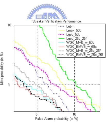
Fig. 2.3 shows the Detection Error Tradeoff (DET) curves [Martin 1997] obtained by evaluating the above systems using the “Test” subset, where Fig. 2.3(a) compares the WGC-based approach and the geometric mean approach, while Fig. 2.3(b) compares the WAC-based approach and the arithmetic mean approach. From the figure, we observe that all the WGC-based LR systems outperform the baseline LR systems “Lubm”, “Lmax_50c”, “Lgeo_50c”, and “Lgeo_25c_25f”, while all the WAC-based LR systems outperform the baseline LR systems “Lubm”, “Lari_50c”, and “Lari_25c_25f”. From Fig. 2.3(a), we observe that “Lgeo_25c_25f” yields the poorest performance. This is because the heuristic geometric mean can produce some singular scores if any cohort model λi is poorly matched with the

input utterance U, i.e., p(U| λi) → 0. In contrast, the results show that the WGC-based LR

systems sidestep this problem with the aid of the weighted strategy. Figs. 2.3(a) and 2.3(b) also show that “WGC_EMVE_w_50c”, “WGC_EMVE_w_25c_25f”, and “WAC_EMVE_w_25c_25f” outperform “WGC_MVE_w_50c”, “WGC_MVE_w_25c_25f”, and “WAC_MVE_w_25c_25f”, respectively. However, ther

een “WAC_MVE_w_50c” and “WAC_EMVE_w_50c”.

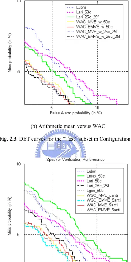
In addition to the above systems, we also evaluated the WAC- and WGC-based LR measures using the hybrid anti-model defined in Eq. (2.4). The hybrid anti-model comprised five conventional anti-models extracted from “Lubm”, “Lmax_50c”, “Lgeo_50c”, “Lari_50c”, and “Lari_25c_25f”. Note that the anti-model of “Lgeo_25c_25f” was not included because of its p

a) Using WAC and gradient-based MVE training (“WAC_MVE_5anti”), b) Using WGC and gradient-based MVE training (“WGC_MVE_5anti”), c) Using WAC and EMVE training (“WAC_EMVE_5anti”), and

DET curves. Clearly, all the hybrid anti-model s using either WAC or WGC methods outperform any baseline LR system with a ngle anti-model.

d) Using WGC and EMVE training (“WGC_EMVE_5anti”).

Fig. 2.4 compares the performance of the hybrid anti-model systems with all the baselines systems, evaluated on the “Test” subset in

system si

(b) Arithmetic mean versus WAC

Fig. 2.3. DET curves for the “Test” subset in Configuration II.

Fig. 2.4. Hybrid anti-model systems versus all baselines: DET curves for the “Test” subset in Configuration II.

B. Discussion

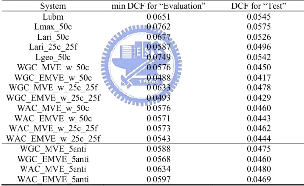
Table 2.3 summarizes the above experiment results in terms of the DCF, which reflects the performance at a specific operating point on the DET curve. For each baseline system, the value of the decision threshold θ was carefully tuned to minimize the DCF in the “Evaluation” subset, and then applied to the “Test” subset. However, the decision thresholds of the proposed WAC- and WGC-based LR measures were optimized automatically using the “Evaluation” subset, and then applied to the “Test” subset.

Table 2.3. DCFs for the “Evaluation” and “Test” subsets in Configuration II. System min DCF for “Evaluation” DCF for “Test”

Lubm 0.0651 0.0545 Lmax_50c 0.0762 0.0575 Lari_50c 0.0677 0.0526 Lari_25c_25f 0.0587 0.0496 Lgeo_50c 0.0749 0.0542 WGC_MVE_w_50c 0.0576 0.0450 WGC_EMVE_w_50c 0.0488 0.0417 WGC_MVE_w_25c_25f 0.0633 0.0478 WGC_EMVE_w_25c_25f 0.0493 0.0429 WAC_MVE_w_50c 0.0576 0.0460 WAC_EMVE_w_50c 0.0571 0.0443 WAC_MVE_w_25c_25f 0.0573 0.0462 WAC_EMVE_w_25c_25f 0.0543 0.0444 WGC_MVE_5anti 0.0588 0.0475 WGC_EMVE_5anti 0.0568 0.0460 WAC_MVE_5anti 0.0634 0.0480 WAC_EMVE_5anti 0.0597 0.0469

Several conclusions can be drawn from Table 2.3. First, all the proposed WAC- and WGC-based LR systems with either the hybrid anti-model or the background model set (the world model plus a cohort) outperform all the baseline LR systems. Second, the performances of the proposed systems using the background model set are slightly better than those achieved using the hybrid anti-model. Third, the performances of the WAC- and WGC-based