國 立 交 通 大 學
土木工程學系
博士論文
載具沿滑軌運動之傾墜分析
Dynamic Analyses of a Vehicle Moving along a Guideway
with Considering the Tip-off Effect
研 究 生: 周勝男
指導教授: 黃炯憲 博士
鄭復平 博士
載具沿滑軌運動之傾墜分析
Dynamic Analyses of a Vehicle Moving along a Guideway
with Considering the Tip-off Effect
研 究 生: 周勝男
Student :
Sheng-Nan Chou
指導教授: 黃炯憲
Advisors :
Chiung-Shiann Huang
鄭復平
Fu-Ping Cheng
國 立 交 通 大 學
土 木 工 程 學 系
博 士 論 文
A Dissertation
Submitted to Department of Civil Engineering
College of Engineering
National Chiao Tung University
in partial Fulfillment of the Requirements
for the Degree of
Doctor of Philosophy
in
Civil Engineering
June 2012
Hsinchu, Taiwan, Republic of China
載具沿滑軌運動之傾墜分析
學生:周勝男
指導教授:黃炯憲 博士
鄭復平 博士
國立交通大學土木工程學系 博士班
摘 要
本研究考量載具與滑軌間的結構互制行為,發展半解析方法分析載具沿著滑軌運 動的傾墜反應。對於飛彈發射系統設計而言,精確的計算其傾墜反應是極為重要的課 題,飛彈可視為本研究之載具。本文提出 R.E. 與 E.E. 兩種模型進行動態反應分析。其 中 R.E. 模型係將載具視為剛性梁,滑軌視為彈性梁,而在 E.E. 模型中將載具與滑軌皆 視為彈性梁。在上述分析模型的解析時,皆考慮了慣性力、科氏力與離心力的影響, 同時載具與滑軌之間皆透過兩個剛性滑腳來接觸。 本研究基於 Euler-Bernoulli 梁理論,採用振態疊加法與拉格蘭日乘子法來推導載 具與滑軌運動的控制方程式。此系統的運動方程式是由一組非線性的微分方程式所 組成,其數值解採用 Petzold-Gear 的後向微分法(Backward Differentiation Formula, BDF)來求算此動態系統的數值模擬結果,所需花費時間較少於一般傳統逐步數值積 分的方法,對於載具與滑軌的分析模擬經與文獻實際特殊案例的結果比較,可呈現本 研究所提出之方法的優點。 利用此分析方法進一步探討滑軌的長度、載具滑腳的距離、載具與滑軌的質量比 與剛性比等各參數對載具傾墜反應的影響,經由本研究之成果,於載具發射系統設計 時,可以提供非常有價值的資訊。 關鍵字: 移動荷重; 移動梁; 拉格蘭日法; 振態疊加法; 傾墜效應Dynamic Analyses of a Vehicle Moving along
a Guideway with Considering the Tip-off Effect
Stduent : Sheng-Nan Chou Advisors : Dr. Chiung-Shiann Huang Dr. Fu-Ping Cheng
Department of Civil Engineering National Chiao Tung University
A
BSTRACT
A semi-analytical solution for analyzing the tip-off responses of a vehicle moving along a guideway is developed by considering the dynamic interaction between the vehicle and the guideway. Accurately determined tip-off responses are important for designing a launch system for a missile, in which the missile can be treated as the vehicle in the present study. Two models are proposed to determine those dynamic responses, namely, R.E. model and E.E. model. In the R.E. model, the vehicle is as-sumed rigid and its guideway is modeled as a flexible beam, while both of the vehicle and guideway are modeled as flexible beams in the E.E model. The inertia, Coriolis, and centrifugal forces are considered in these models. The vehicle contacts with its guideway through two rigid shoes.
Equations for governing the motions of the vehicle and the guideway are devel-oped using the Lagrangian approach and the modal superposition method, on the basis of the Euler-Bernoulli beam theory. The governing equations, which are a set of nonlinear differential equations, are solved by the Petzold-Gear backward differentia-tion formula numerical method. It takes time lower than the tradidifferentia-tional step-by-step numerical integration methods. Comparisons of the presented solutions with those based on different published models for the vehicle and guideway reveal the advan-tages of the present approach.
The solutions are further employed to investigate the effects of the length of the guideway, distance between the shoes of the vehicle, and mass and rigidity ratios of
the vehicle to the guideway on the tip-off responses of the vehicle. The results pre-sented herein provide valuable information for designing vehicle launch systems.
keywords: moving load; moving beam model; Lagrangian approach; mode superpo-sition; tip-off effect.
A
CKNOWLEDGEMENTS
年過半百拿到博士學位,心中的喜樂絕對不比一般的年輕學子低,除了全職的上 班工作與出差外,論文投稿與寫作期間的日常生活幾乎就是晚上窩在電腦前絞盡腦汁 的推導理論與寫程式度過,雖然辛苦,但是收穫卻特別多。回想交大的求學階段,遇 到許多的貴人,首先必須感謝我的指導老師鄭復平博士,您亦師亦友多年來持續在生 活上的關心與論文研究上的指導,直到老師退休還熱心的將我託付給指導老師黃炯憲 博士,使得我在最後關頭還能在研究上找到方向並總結出重要的成果,由於上班的任 務繁重與限制,多次有勞黃老師假日來學校指導論文瓶頸與英文論文寫作,兩位指導 老師的研究精神讓我如沐春風受益良多,當學生的我在此衷心感謝,期待日後仍能繼 續向老師們多方請益。 在求學期間,劉俊秀、林昌佑、王彥博、洪士林、趙文成與陳誠直等諸位老師的 學識淵博,讓我藉著修課與討論增加了專業的本質學能,同時在博士班資格考時的研 究方向指導,讓我獲得許多寶貴的知識,在此一併致謝。由於工作上與學業上的壓力 交雜,曾經萌生放棄學業的念頭,在此要感謝我生命中的貴人與長官姜武英博士,總 是在每個階段引領我走出低潮,同時費心協助我選定的論文題目能夠與工作上的任務 應用做完美的結合,讓我在工作與學業上能取得最佳的平衡並堅持到底。在畢業論文 口試時,非常感謝楊明放院長、姚忠達教授與上述諸位老師的費心指導,並提供許多 寶貴的建議與修訂方向,讓這份研究成果更為完整,在此表達衷心的謝忱。 我的高中同窗好友與同事李運璋博士,不僅協助我突破許多研究上的理論瓶頸, 還引導我進入 LATEX 排版與 Beamer 簡報系統等論文寫作工具的大門,由於我對文件 品質上的執著,非常感謝他的耐心指導陪我走過初學階段。此外,林仁正學長多年來 在每一段時間都會來電關切我的研究進度,雖然備感壓力,但是非常窩心,謝謝您學 長。攻讀博士學位是我人生中非常重要的階段,我很幸運擁有一個非常美滿的家庭, 女兒項萱與兒子揚賀在成長與求學階段都能自我管理的很好,讓我不僅無後顧之憂甚 至以他們為榮;當然最重要的是我摯愛的妻子淑敏,她為我承擔了大部分的家務與孩 子們的瑣事,是我能夠畢業的最大支柱,一世夫妻百世恩,在求學的低潮期感謝她溫 馨的陪我走過艱辛歲月,在論文即將付梓之際,我很願意將這份成果與我親愛的家人 們共享,由於無法逐一感謝曾經幫助過我的每一個人,謹以誠摯的心向大家致上最真 誠的謝意!
周勝男
謹識 07/10/2012T
ABLE
OF C
ONTENTS
Abstract(Chinese) i
Abstract(English) ii
Acknowledgements iv
Table of Contents viii
List of Tables ix
List of Figures xiii
Notation xiv
1 Introduction 1
1.1 Background and Motivation . . . 1
1.2 Statement of the Problems . . . 2
1.3 Literature Review . . . 3
1.4 Objectives, Approach and Research Coverage . . . 8
1.5 Dissertation Outline . . . 9
2 A rigid vehicle moving along an inclined rigid guideway 12 2.1 Theory and Formulation . . . 12
2.2 Two-shoe contact phase . . . 14
2.4 Numerical examples and parametric study . . . 21
2.4.1 Influence of angle of inclination of guideway . . . 23
2.4.2 Influence of length of guideway . . . 25
2.4.3 Influence of distance between shoes of vehicle . . . 26
3 A rigid vehicle moving along an inclined flexible guideway 29 3.1 Mathematical modeling behaviors of a guideway . . . 29
3.1.1 Position history of vehicle . . . 31
3.1.2 Two-shoe contact phase . . . 31
3.1.3 Tip-off phase . . . 36
3.2 Calculation of dynamic response of guideway . . . 38
3.3 Modelling the dynamic responses of vehicle at tip-off . . . 42
3.4 Numerical validation and examples . . . 47
3.4.1 Case 1: Displacement of contact points between vehicle and guide-way . . . 47
3.4.2 Case 2: Comparison between tip-off results of rigid and pseudo-rigid guideways . . . 48
3.4.3 Case 3: Behavior of rigid vehicle on elastic guideway . . . 50
3.5 Parametric study . . . 54
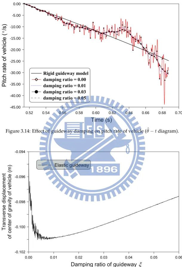
3.5.1 Influence of damping ratio of guideway . . . 54
3.5.2 Influence of angle of inclination of guideway . . . 59
3.5.3 Influence of length of guideway . . . 61
3.5.4 Influence of distance between shoes of vehicle . . . 63
3.5.5 Influence of Coriolis force and centrifugal force . . . 66
3.5.6 Influence of guideway length and distance between the shoes . . 68
4 A flexible vehicle moving along an inclined flexible guideway 72 4.1 Theory and Formulation . . . 72
4.1.2 Two-shoe contact phase . . . 73
4.1.3 Tip-off phase . . . 81
4.1.4 Dynamic responses of vehicle and guideway . . . 83
4.2 Numerical validation and examples . . . 86
4.2.1 Case 1: displacement of contact points between vehicle and guide-way . . . 87
4.2.2 Case 2: Two shoes constraint condition verification . . . 88
4.2.3 Case 3: A rigid vehicle moves along a rigid guideway . . . 89
4.2.4 Case 4: A rigid vehicle moves along an elastic guideway . . . 93
4.2.5 Case 5: An elastic vehicle moves along an elastic guideway . . . 95
4.3 Parametric Study . . . 98
4.3.1 Influence of length of guideway . . . 98
4.3.2 Influence of distance between shoes of vehicle . . . 99
4.3.3 Influence of mass ratio and flexural rigidity ratio . . . 101
5 Conclusions and Future works 105 5.1 Conclusions . . . 105
5.2 Future works . . . 107
Bibliography 112 A Appendix 113 A.1 Derivation of eHia, eHib, eHic, eHid. . . 113
L
IST
OF T
ABLES
1.1 Three types analytical models used for vehicle launch. . . 11
2.1 Parameters of the vehicle launch system. . . 22
3.1 Parameters of the vehicle launch system. . . 50 3.2 Comparison of pitch angles for pseudo-rigid guideway and rigid
guide-way. . . 51 3.3 Comparison of pitch rates for pseudo-rigid guideway and rigid guideway. 51 3.4 Comparison of dynamic responses between elastic guideway model with
different damping ratios and rigid guideway model. . . 55 3.5 Effect of distance between the shoes on maximum difference in dynamic
response of vehicle. . . 66 3.6 Effect of Coriolis and centrifugal forces on dynamic response of vehicle. 67
4.1 Parameters of the vehicle launch system. . . 86 4.2 Comparison of pitch angles of vehicle obtained using different models. . 89 4.3 Comparison of pitch rates of vehicle obtained using different models. . . 89 4.4 Combinations of flexural rigidities of vehicle and guideway. . . 99
L
IST
OF F
IGURES
1.1 A typical vehicle launch system in a two-shoe contact phase. . . 2
1.2 A typical vehicle launch system in a tip-off phase. . . 3
2.1 A typical rigid guideway used for rigid vehicle launch. . . 12
2.2 A typical real thrust-time curve. . . 13
2.3 A typical thrust-time curve to simulate. . . 13
2.4 Motion of vehicle in tip-off phase. . . 18
2.5 Pitch angle ¯θ− t of vehicle on rigid guideway. . . 22
2.6 Pitch rate ˙¯θ− t of vehicle on rigid guideway. . . 23
2.7 Effect of angle of inclination on pitch angle of vehicle (¯θ− θE diagram). . 24
2.8 Effect of angle of inclination on pitch rate of vehicle ( ˙¯θ− θE diagram). . . 24
2.9 Effect of guideway length on pitch angle of vehicle (¯θ− L diagram). . . . 25
2.10 Effect of guideway length on pitch rate of vehicle ( ˙¯θ− L diagram). . . . 26
2.11 Effect of distance between the shoes of the vehicle on pitch angle of vehicle (¯θ− d diagram). . . 27
2.12 Effect of distance between the shoes of the vehicle on pitch rate of vehi-cle ( ˙¯θ− d diagram). . . 27
3.1 A typical flexible guideway used for rigid vehicle launch. . . 29
3.2 Free-body diagrams of a vehicle and its guideway. . . 30
3.3 Typical displacements of vehicle and its guideway. . . 30
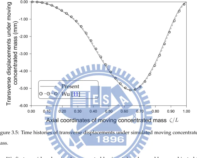
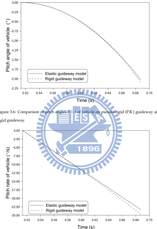
3.5 Time histories of transverse displacements under simulated moving con-centrated mass. . . 47 3.6 Comparison of pitch angles ¯θ−t of vehicle on pseudo-rigid (P.R.)
guide-way and rigid guideguide-way. . . 49 3.7 Comparison of pitch rates ˙¯θ− t of vehicle on pseudo-rigid (P.R.)
guide-way and rigid guideguide-way. . . 49 3.8 Transverse displacement of vehicle’s center of gravity. . . 52 3.9 Transverse velocity of vehicle’s center of gravity. . . 52 3.10 Comparison of pitch angles of vehicle on elastic guideway and rigid
guideway. . . 53 3.11 Comparison of pitch rates of vehicle on elastic guideway and rigid
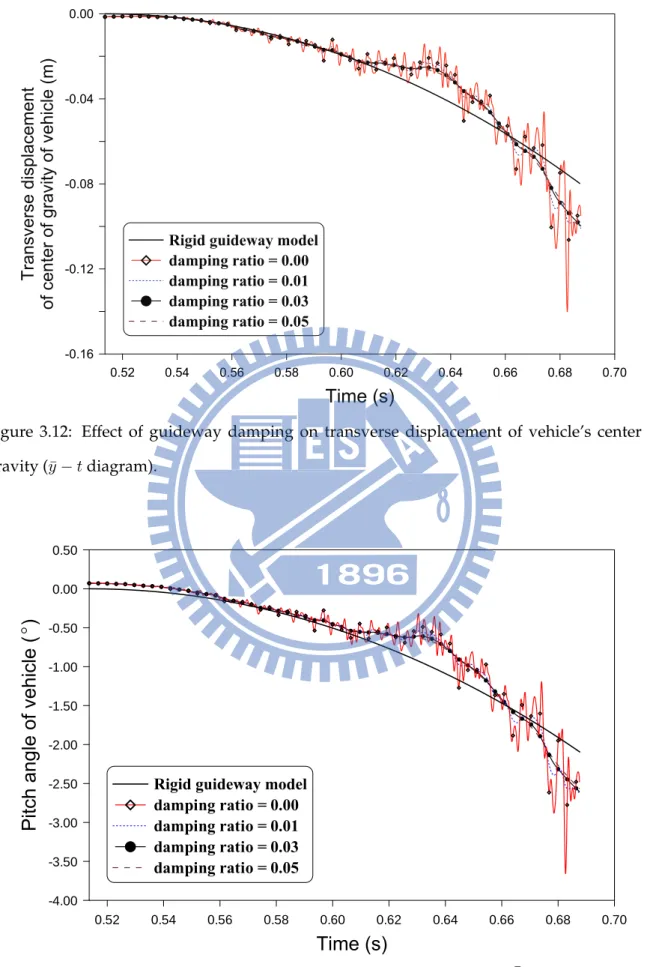
guide-way. . . 53 3.12 Effect of guideway damping on transverse displacement of vehicle’s
center of gravity (¯y− t diagram). . . 56
3.13 Effect of guideway damping on pitch angle of vehicle (¯θ− t diagram). . 56
3.14 Effect of guideway damping on pitch rate of vehicle ( ˙¯θ− t diagram). . . 57
3.15 Effect of guideway damping on transverse displacement of vehicle’s center of gravity (¯y− ξ diagram). . . 57
3.16 Effect of guideway damping on pitch angle of vehicle (¯θ− ξ diagram). . 58
3.17 Effect of guideway damping on pitch rate of vehicle ( ˙¯θ− ξ diagram). . . 58
3.18 Effect of angle of inclination on transverse displacement of vehicle’s center of gravity (¯y− θE diagram). . . 59 3.19 Effect of angle of inclination on pitch angle of vehicle (¯θ− θE diagram). . 60 3.20 Effect of angle of inclination on pitch rate of vehicle ( ˙¯θ− θE diagram). . . 61 3.21 Effect of guideway length on transverse displacement of vehicle’s center
of gravity (¯y− L diagram). . . 62
3.22 Effect of guideway length on pitch angle of vehicle (¯θ− L diagram). . . . 62
3.24 Effect of distance between the shoes of the vehicle on transverse
dis-placement of vehicle’s center of gravity (¯y− d diagram). . . 64
3.25 Effect of distance between the shoes of the vehicle on pitch angle of vehicle (¯θ− d diagram). . . 65
3.26 Effect of distance between the shoes of the vehicle on pitch rate of vehi-cle ( ˙¯θ− d diagram). . . 65
3.27 Effect of Coriolis and centrifugal forces on displacement of vehicle’s center of gravity (¯y− t diagram). . . 67
3.28 Effect of Coriolis and centrifugal forces on pitch angle of vehicle (¯θ− t diagram). . . 68
3.29 Effect of Coriolis and centrifugal forces on pitch rate of vehicle ( ˙¯θ − t diagram). . . 69
3.30 Effect of guideway length and distance between shoes on pitch angle of vehicle: (a) 3D plot (b) contour plot. . . 70
3.31 Effect of guideway length and distance between shoes on pitch rate of vehicle: (a) 3D plot (b) contour plot. . . 71
4.1 A typical flexible guideway used for flexible vehicle launch. . . 72
4.2 Free-body diagrams of a vehicle and its guideway. . . 73
4.3 Free body diagrams of vehicle in tip-off phase. . . 81
4.4 Time histories of transverse displacements under simulated moving con-centrated mass. . . 87
4.5 Verification of constraint conditions of the two shoes of the vehicle rela-tive to the guideway. . . 90
4.6 Verification of acceleration constraint using different numbers of modes. 91 4.7 Comparisons of pitch angles θ − t of vehicle obtained using different models. . . 92 4.8 Comparisons of pitch rates ˙θ−t of vehicle obtained using different models. 92
4.9 Comparisons of pitch angles θ − t of vehicle obtained using different models and formulations. . . 94 4.10 Comparisons of pitch rates ˙θ−t of vehicle obtained using different
mod-els and formulations. . . 94 4.11 Comparisons of pitch angles of vehicle obtained using different
num-bers of modes. . . 96 4.12 Comparisons of pitch angles of vehicle obtained using different time
increment. . . 96 4.13 Comparison of pitch angles of vehicle obtained using different models. . 97 4.14 Comparison of pitch rates of vehicle obtained using different models. . . 97 4.15 Effect of length of guideway on pitch angle of vehicle at take-off (θ− Lg
diagram). . . 100 4.16 Effect of length of guideway on pitch rate of vehicle at take-off ( ˙θ− Lg
diagram). . . 100 4.17 Effect of distance between shoes of vehicle on pitch angle of vehicle at
take-off. . . 102 4.18 Effect of distance between shoes of vehicle on pitch rate of vehicle at
take-off. . . 102 4.19 Effect of mass ratio and flexural rigidity ratio on pitch angle of vehicle:
(a) 3D plot (b) contour plot. . . 103 4.20 Effect of mass ratio and flexural rigidity ratio on pitch rate of vehicle:
N
OTATION
P(t) Thrust force acting on vehicle
J Mass moment of inertia of rigid vehicle
g Gravitational acceleration
θE Angle of inclination of guideway
EvIv Flexural rigidity of vehicle
EgIg Flexural rigidity of guideway
Lv Length of vehicle
Lg Length of guideway
ξv Damping ratio of vehicle
ξg Damping ratio of guideway
ρvAv Mass per unit length of vehicle
ρgAg Mass per unit length of guideway
mv Mass of vehicle
d Distance between shoes of vehicle
d1 Distance between the rear shoe and the center of gravity of the vehicle
dR Distance between left end to rear shoe of vehicle
dG Distance between left end to center of gravity of vehicle
dF Distance between left end to front shoe of vehicle
F (t) Front shoe contact forces between vehicle and guideway
R(t) Rear shoe contact forces between vehicle and guideway
ζ(t) Position coordinate of vehicle on guideway ˙
ζ(t) Velocity of vehicle on guideway ¨
ζ(t) Acceleration of vehicle on guideway
ζR Distance from left end of guideway to rear shoe of vehicle at t = 0
tb Time of thrust build-up
tF Time at which front shoe of vehicle loses contact
tR Time at which vehicle takes-off
w(ζ, t) Displacements of the shoe contact point in the y-direction of the
guideway at position ζ and time t
yR Displacements of the rear shoe contact point in the y-direction of the guideway
yF Displacements of the front shoe contact point in the y-direction of the guideway
¯
y (t) Displacement of the vehicle’s center of gravity at time t
¯
θ (t) Pitch angle of the vehicle’s center of gravity at time t
˙¯
y (t) Velocity of the vehicle’s center of gravity at time t
˙¯
θ (t) Pitch rate of the vehicle’s center of gravity at time t
Yi(t) Generalized coordinate corresponding to the ith mode ˙
Yi(t) Generalized velocity corresponding to the ith mode ¨
Yi(t) Generalized acceleration corresponding to the ith mode
Y Matrix of generalized coordinate
˙
Y Matrix of generalized velocity
¨
Y Matrix of generalized acceleration
M Matrix of generalized mass
C Matrix of generalized damping
K Matrix of generalized stiffness
Q Matrix of generalized force
G1 Displacement constraint at rear shoe of vehicle
G2 Displacement constraint at front shoe of vehicle
λ Lagrange multiplier
Mr Mass ratio between vehicle and guideway
C
HAPTER
O
NE
Introduction
1.1
Background and Motivation
In real designs of all vehicle launch systems, one of the main concerns is to mini-mize the transverse motions of the vehicle, which can be a missile, moving along its guideway, especially when the vehicle takes off. In the field of control engineering, a vehicle and its guideway are typically modeled as rigid bodies for the tip-off analy-sis. Although such modeling is quite simple and easily used, it does not consider the dynamic interactions between the vehicle and its guideway. To reduce the transverse motions of the vehicle, it is important to accurately consider the vehicle acting forces and the associated vehicle-guideway interactions during the launch phase.
At present, much research has been devoted to the structural dynamic analysis of a flexible flight vehicle, whereas until now there has been no investigated study for vehicle launch system design considering the vehicle and guideway as flexible bod-ies in real applications. The bending flexibilitbod-ies of vehicle and guideway can have a remarkable influence on the behaviors of the vehicle as it leaves the guideway of launcher, and hence on the resulting accuracy of control. The responses of the ve-hicle at take-off significantly affect its flight control, and accurately determining the responses of the vehicle in the tip-off phase is crucial. The motivation of this study is to develop an analysis method to efficiently and accurately study dynamic behaviors of a vehicle-guideway system with time-dependent constraints between the vehicle
and the guideway.
1.2
Statement of the Problems
When a vehicle moves along the guideway, the vehicle is mainly subjected to thrust, inertia, and gravity forces, and two phases can be identified (see Fig. 1.1). Before the front shoe of the vehicle loses contact with the guideway, the vehicle is in a two-shoe contact phase (see Fig. 1.1). The vehicle rotates with respect to its rear two-shoe when its front shoe loses contact with the guideway, and this phenomenon is known as tip-off. When the vehicle exhibits tip-off, it is referred to as being“in the tip-off phase” (see Fig. 1.2). In the published literature, such a vehicle and its guideway are typically modeled as rigid bodies for the tip-off analysis, the model is not sufficiently accurate to present the real behaviors of the vehicle. In real applications, the mass of the launched vehicle substantially exceeds that of its guideway, and both of the vehicle and the guideway are flexible.
Figure 1.2: A typical vehicle launch system in a tip-off phase.
It is very important to accurately determine the behaviors of the vehicle When the vehicle excessively moves in the transverse direction during take-off, it is very possible that the vehicle collides with the guideway system. When the velocity of a vehicle is too low to develop the aerodynamic force for controlling its attitude or direction during the tip-off phase, its control fins can not function well, and the balance between the aerodynamic and other forces do not yet reach a stable state. Therefore, the control fins must be locked during the initial trajectory, and the initial flight conditions, which mainly result from the behaviors of the vehicle in the tip-off phase, must be accurately determined.
1.3
Literature Review
The dynamic responses of a beam subjected to a moving vehicle (or structure) have at-tracted the attention of researchers for a long time. An excellent state-of-the-art review
is given by the subcommittee on vibration problems associated with flexural member on transit systems [1]. The moving vehicle is often modeled as a moving force, a mov-ing mass, a movmov-ing oscillator (also called a sprung mass model) or a movmov-ing beam. Modeling as a moving force is the simplest and oldest approach, which neglects the interaction between the vehicle and the beam [2–6]. Research work on this topic can be traced back to the 19thcentury [2]. Timoshenko [3] derived numerous approximate solutions to the problem of a simply-supported beam under moving loads. Ayre et
al. [4] studied the transverse vibrations of a two-span beam under a moving constant
force. The moving force model is well known to apply only to the case in which the mass of the moving vehicle is much smaller than that of the beam, and only when the dynamic responses of the moving vehicle are not of interest. N. Sridharan et al. [5] presented a numerical analysis of vibration of beams subjected to moving loads. Numerical results obtained for the case of a constant force moving over a uniform simply supported beam have been compared with those obtained by using the analyt-ical method. Hamada [5] has been presented a method , based on the double Laplace transformation, for dynamic analysis of a simply supported and damped Bernoulli-Euler uniform beam of finite length subjected to the action of a moving concentrated force. K. Henchi et al. [6] developed an exact dynamic stiffness element under the frame work of finite element approximation is presented to study the dynamic re-sponse of multi-span structures under a convoy of moving loads.
A moving mass model is a simple model that to some extent accounts for the in-teraction between the dynamic inin-teraction between a moving structure and a beam [7–11]. The model was first proposed by Jeffcott [7] in 1929. Stani˘si´c [8] employed the Fourier technique to investigate the responses of beams to an arbitrary number of concentrated moving masses. Akin and Mofid [9] presented a numerical solution by using the separation of variables technique to analyze the dynamic responses of an Euler-Bernoulli beam to a moving mass. Their solution scheme was very simple and can be used to determine the responses of beams under various boundary conditions.
Cifuentes [12] presents a combined finite element/finite difference technique to deter-mine the response of a beam excited by a moving mass. The technique introduced herein is based on a Lagrange Multiplier formulation that allows one to represent the compatibility condition at the beam/mass interface using a set of auxiliary functions. This approach can be easily adapted to a standard finite element code. Michaltsos
et al. [13] studied the linear dynamic response of a simply supported uniform beam
under a moving load of constant magnitude and velocity by considering the effect of its mass. They highlighted the importance of considering the effect of the load mass. As the ratio M/ml (moving mass/mass of beam) increases, depending on the velocity, the ratio wM/wP (displacement of moving mass/displacement of load because of mov-ing force) can increase considerably. Lee [14] studied the equation of motion in matrix form for an Euler beam acted upon by a concentrated mass moving at a constant speed is formulated by using the Lagrangian approach and the assumed mode method. Lee [15] also analysed extensively the transverse vibration of a Timoshenko beam acted on by an accelerating mass and compared with the corresponding behaviour of a Tim-oshenko beam subjected to an equivalent moving force neglecting the inertial effects of the mass. The effects of prescribed values of constant acceleration or deceleration of the moving mass on the deflection under the moving mass, as well as the contact forces, are investigated. Michaltsos [16] also studied the linear dynamic response of a simply supported elastic single-span beam under a moving load of constant magni-tude and variable velocity, with an emphasis on the effect of acceleration or deceler-ation on the behaviour of the beam under a single load, or an actual vehicle model. Dehestani et al. [10] showed that it is necessary to consider the Coriolis acceleration associated with a mass moving along a vibrating beam. Wu [11] examined the effects of the inertial, Coriolis, and centrifugal forces induced by non-coupled moving masses on the dynamic responses of an inclined simply-supported beam. Further, Frýba [17] compiled a book containing descriptions of almost all studies on the vibration of solids and structures under a moving load.
A moving oscillator model includes mass, springs and dampers to capture the real dynamic characteristics of a moving vehicle. It is more complicated than a mov-ing mass model [18–20]. Biggs [18] presented a semi-analytical solution to the prob-lem of a sprung mass moving on a simply-supported beam. Using a series expansion technique, Pesterev et al. [19] examined the responses of an elastic continuum to mul-tiple moving oscillators. Yang et al. [20] proposed a vehicle-bridge interaction element (VBI) to investigate the vibrations of simply-supported beams during the passage of high-speed trains.
The vehicle-bridge interaction dynamics has been also extensively studied for ap-plication to high-speed railways [21–28]. In particular, Yang et al. [21] investigated the vibration of simple beams during the passage of high-speed trains. Cojocaru et al. [27] studied the vibrations of an elastic bridge loaded by a second elastic beam moving with a constant speed. Zhang et al. [24] proposed a space model for train carriages and introduced a dynamic analysis for train-bridge interaction. Delgado and dos Santos [22] modeled the railway bridge-vehicle interaction on high-speed tracks.
Unlike a moving oscillator model, which treats a moving vehicle as a discrete sys-tem, a moving beam model considers a vehicle as a continuum and represents it as a beam. Cojocaru et al. [27] first studied the vibrations of an elastic bridge loaded by a second elastic beam that moved along the bridge at a constant speed. The vehicle was assumed to be connected to the bridge by means of a rigid interface. The quasi-static deformation of the bridge was obtained through the Laplace transform, while the dy-namic responses of the bridge were determined via the Galerkin method. Delgado and dos Santos [22] modeled the railway bridge-vehicle interaction on high-speed tracks. The action of railway traffic on bridges is considered as a set of moving masses, being the effects of the moving forces and masses implied. Zhang et al. [29] investigated the dynamic responses of a simply-supported beam on which was moving an elastic beam at a constant speed using the modal superposition method. The model consisted of two Euler-Bernoulli beams that were connected by flexible springs at two points, so
that the interactive forces between the simply-supported beam and the moving beam were easily found from the relative deflection of the two points. A small rotation an-gle in rigid body motions was assumed. They developed a set of linear differential equations for the motions of two beams. Sreeram et al. [30] employ the Lagrangian multiplier technique to develop a h-p version finite element model for a certain class of dynamics problems. Variational principle is the basis of this formulation with es-sential conditions applied via Lagrangian multipliers. The example considered here is a problem of a beam moving over supports. Lagrangian multiplier implementation of the problem with finite element technique, is very effective compared to other global methods such as assumed mode technique. Kim [31] investigate the vibration and stability of an infinite Bernoulli-Euler beam resting on a Winkler-type elastic founda-tion when the system is subjected to a static axial force and a moving load with ei-ther constant or harmonic amplitude variations. Chen et al. [32] investigates dynamic stability in transverse parametric vibration of an axially accelerating viscoelastic ten-sioned beam. The beam is described by the Kelvin model, and the Galerkin method is applied to discretize the governing equation into a infinite set of ordinary-differential equations under the fixed-fixed boundary conditions. Fung et al. [33] studied a flexible beam slides in and out of the rigid wall. The equations of motion for a deploying beam with a tip mass are derived by using Hamilton’s principle. Four dynamic models: Tim-oshenko, Euler, simple-flexible and rigid-body beam theories are used to describe the axially moving beam.
All of the aforementioned studies mainly focused on the dynamic responses of beams and were applicable to the design of railroad tracks, railroad bridges, and high-way bridges. Relatively few studies focused on the dynamic behaviors of a vehicle, such as a missile, when the vehicle moves along the guideway, which can represent a launcher system (see Fig. 1.1). Analyses of various aspects of flexible vehicle behav-ior in free flight or with time-dependent constraints have appeared frequently in the literature. The interaction between the vehicle and its guideway differs considerably
between the two-shoe contact phase and the tip-off phase, and the vehicle displays very different behaviors. Consequently, the corresponding dynamic responses of the vehicle have to be modeled in these two phases.
1.4
Objectives, Approach and Research Coverage
Because the responses of the vehicle at take-off significantly affect the flight control of the vehicle, accurately determining the responses of the vehicle in the tip-off phase is crucial. This study applied the models of rigid vehicle and rigid guideway (R.R. model) [34], rigid vehicle and elastic guideway (R.E. model) [35], and elastic vehicle and elastic guideway (E.E. model) [36] for tip-off analysis of the vehicle at take-off.
In the R.E. model, the vehicle and the guideway are modeled as a rigid free-free beam and an inclined elastic simply-supported beam, respectively. The flexible guide-way is assumed to be Euler-Bernoulli beam. The vehicle is connected to the guideguide-way through two points of contact, which are considered to be rigid connections, so that their dynamic responses are the same during vehicle take-off. The equations of motion for the vehicle and its guideway, in terms of functions of the configuration coordinates and time, are established via the Newton’s second law based on the free body diagram of the vehicle with appropriate displacement constraints.
In the E.E. model, the guideway is modeled as an inclined simply-supported uni-form flexible beam, and the vehicle is treated as a flexible free-free beam under a pre-specified thrust force. Equations for governing the motions of the vehicle and the guideway are developed using the Lagrangian approach and the assumed mode method, on the basis of the Euler-Bernoulli beam theory. The governing equations take into account the inertia, Coriolis, and centrifugal forces that are induced by the vehicle as well as the dynamic interaction between the vehicle and its guideway. Table 1.1 summarizes the comparisons among the three models.
To solve for the governing equations in the R.E. model and E.E. model, a modal superposition technique is adopted to convert the governing equations, which are
nonlinear partial differential equations, into a set of nonlinear first-order differential equations with time as the independent variable. Then, the Petzold-Gear backward differentiation formula (BDF) numerical method [37] is employed to solve these first-order differential algebraic equations (DAEs). The proposed solutions are validated by comparing the results with published results obtained from models of a rigid vehicle on a rigid guideway. The effects of the length of the guideway, distance between the shoes of the vehicle, and mass and flexural rigidity ratios of the vehicle to the guide-way upon tip-off of the vehicle are thoroughly studied. The results presented here provide valuable information for designing vehicle launch systems.
1.5
Dissertation Outline
The contents of the dissertation are organized as:
Chapter 1 describes the relevant literature review, the motivation and main pur-poses of the work.
Chapter 2 presents the R.R. model and re-develops solutions for the governing equations of the model. The equations of motion of the vehicle are derived by New-ton’s second law. The pitch angle and the pitch rate of the vehicle in this model were directly determined from the displacement and velocity of the vehicle at the points of two shoes.
Chapter 3 proposes the R.E. model and develops solutions for the governing equa-tions of the model. Equaequa-tions for governing the motion of the the guideway is derived by taking into account equations for the influences of the inertia force, Coriolis force, and centrifugal force induced by the vehicle as well as the dynamic interaction be-tween the vehicle and its guideway, on the basis of the Euler-Bernoulli beam theory and the assumed mode method. Notably, the pitch angle and the pitch rate of the ve-hicle in this model were indirectly determined from the displacements and velocity of the guideway at the points of contact with the two shoes of the vehicle.
equa-tions of the model. The equaequa-tions of motion for the vehicle and the guideway are de-veloped using the Lagrangian approach and the assumed mode method based on the Euler-Bernoulli hypothesis. Notably, the pitch angle and the pitch rate of the vehicle in this model were directly determined from the displacements and velocity of two shoes of the vehicle.
Chapter 5 shows the conclusions of the present study and suggestions for the future studies.
R.R. Model R.E. Model E.E. Model
Analytical
Method
Calculation
of
T
ip-of
f
Response
Dynamical
Interactions
Linearity
of
Dif
ferential
Equation
Newton’s second law . Newton’s second law . Mode superposition. Displacement compatibility . Newton’s second law . Mode superposition. Lagrangian multiplier . Dir ect calculation. Indir ect calculation. Dir ect calculation.No. Yes. Yes.
Linear second or der O.D.E. Nonlinear second or der P.D.E. Nonlinear second or der P.D.E. T able 1.1: Thr ee types analytical models used for vehicle launch.
C
HAPTER
T
WO
A rigid vehicle moving along an inclined
rigid guideway
2.1
Theory and Formulation
Figure 2.1 schematically depicts a typical guideway for launching a vehicle. The guideway is considered as an inclined fixed rigid beam, while the vehicle is regarded as a rigid beam moving along the guideway under the action of a predetermined thrust force. This model is referred as R.R. model and the derivation of these formulas is based on Yao and Zhang [34].
mv, J ζ(t), ˙ζ(t), ¨ζ(t) θE P (t) R(t) F (t) mvg d1 ζR d ζF x y
The vector of thrust is assumed to be along the vehicle’s centerline (C.L.) and always coincides with the line joining the two contact points (see Fig. 2.1). While the vehicle moves, the two shoes of the vehicle are assumed to slide along the guideway by means of a rigid contact. The thrust force, P (t) in Fig. 2.1, acting on a vehicle is predetermined in real applications. A typical real thrust-time curve is shown in Fig. 2.2. An ideal thrust-time curve in the design is obtained from full scale ground tests for a vehicle booster.
0.0 2.0 4.0 6.0 8.0 10.0 0.00 20000.00 40000.00 60000.00 80000.00
Figure 2.2: A typical real thrust-time curve.
Pmax
P (t)
tb tF tR t
In order to simplify the analyses conducted in this work, we considered a simpli-fied thrust-time curve given in Fig. 2.3, where tb is the thrust build-up time. Normally, the time for the thrust force reaching a steady state is about 100 ms in real design. Pmax is the value of P (t) in the steady state; tF and tR are the times when the vehicle front shoe and rear shoe lose contact with the guideway, respectively. The term tRis called the tip-off time. Between tF and tR, vehicle tip-off occurs.
When such a vehicle moves along a guideway, the vehicle is mainly subjected to the thrust, inertia, and gravity forces, and two different phases can be specified, namely, two-shoe contact phase and tip-off phase. In the two shoe contact phase (cor-responding to 0 ≤ t ≤ tF in Fig. 2.3), the two shoes of the vehicle contact with the
guideway, while in the tip-off phase (corresponding to tF < t ≤ tR in Fig. 2.3), only
the rear shoe contact with the guideway.
From the typical thrust-time curve in Fig. 2.3 and the design parameters of a vehicle and its guideway, one can easily find the position ζ(t) and velocity ˙ζ(t) of the rear shoe (see Fig. 2.1), and tF and tR can be easily determined. Consequently, one is able to identify in which phase the vehicle is at a particular moment.
2.2
Two-shoe contact phase
• When 0 ≤ t ≤ tb :
Based on the aforementioned assumptions and the relationship of geometry in Fig. 2.1, the equations of motion of the vehicle can be written as
mvζ(t) = P (t)¨ − mvg sin θE (2.1)
J ¨θ = F (t) (d− d1)− R(t)d1 (2.3)
where mv and J denote the mass and the mass moment of inertia of the vehicle; d denotes the distance between the front and rear shoes of the vehicle; d1 is the distance
between the rear shoe and the center of gravity of the vehicle; θE is the angle of incli-nation of the guideway; g is the gravitational acceleration; F (t) and R(t) represent the moving loads of the contact points at front shoe and rear shoe, respectively. Assume the system is initially at rest.
From the thrust-time curve in Fig. 2.3 and the design parameters of the vehicle and its guideway, integrating Eq. (2.1) yields ζ(t), ˙ζ(t) and ¨ζ(t)as follows.
¨ ζ(t) = 1 mv ( Pmax tb t− mvg sin θE ) (2.4) ˙ ζ(t) = 1 mv ( Pmax 2tb t 2− m vg sin θE· t ) + ˙ζ(0) (2.5) ζ(t) = 1 mv ( Pmax 6tb t 3− 1 2mvg sin θE · t 2 ) + ˙ζ(0)· t + ζR (2.6) ˙
ζ(0)is the initial velocity of the vehicle and ζ(0) is the x coordinate from the rear shoe of vehicle to the left end of the guideway. When the system is initially at rest ˙ζ(0) = 0 and ζ(0) = ζR.
When t = tb, the thrust reaches steady state, and ˙ζ(tb)and ζ(tb)are given in Eqs.
˙ ζ(tb) = tb mv ( Pmax 2 − mvg sin θE ) (2.7) ζ(tb) = t 2 b mv ( Pmax 6 − 1 2mvg sin θE ) + ζR (2.8)
These values are the initial values of the two-shoe contact phase when thrust force is in steady state.
Before the tip-off phase, the relative motion and rotation in y -direction and pitch direction are zero respectively. As a result, the reaction forces F (t) and R(t) between the vehicle and guideway can be obtained from Eqs. (2.2) and (2.3),
F (t) = d1 dmvg cos θE (2.9) R(t) = ( d− d1 d ) mvg cos θE (2.10)
The reaction forces F (t) and R(t) are constant before the tip-off phase of vehicle.
• When tb < t≤ tF :
When the thrust reaches steady state, two shoes of the vehicle are still constrained by the guideway. The motion of vehicle is governed by,
¨
ζ(t) = 1
mv
Integrating Eq. (2.11) and employing ˙ζ(tb)and ζ(tb)as the initial conditions yields ˙ ζ(t) = 1 mv (Pmax− mvg sin θE)· (t − tb) + ˙ζ(tb) (2.12) ζ(t) = 1 2mv (Pmax− mvg sin θE)· (t − tb) 2+ ˙ζ(t b)· (t − tb) + ζ(tb) (2.13)
When t = tF, just before a vehicle moves into the tip-off phase, ˙ζ(tF)and ζ(tF)of
the vehicle can be obtained from Eqs. (2.14) and (2.15) given in the following,
˙ ζ(tF) = 1 mv (Pmax− mvg sin θE)· (tF − tb) + ˙ζ(tb) (2.14) ζ(tF) = 1 2mv (Pmax− mvg sin θE)· (tF − tb) 2+ ˙ζ(t b)· (tF − tb) + ζ(tb) (2.15)
When ζ(tF) = ζF, and the distance ζF between the front shoe of vehicle at t = 0
and the right end of guideway is predetermined in real application. Substituting ζ(tF)
into Eq. (2.15), one can determine tF from Eq. (2.16) when the front shoe of vehicle
loses contact. Then, substituting tF into Eq. (2.14), one finds ˙ζ(tF)of vehicle.
tF = tb+ mv (Pmax− mvg sin θE) · [√ ˙ ζ(tb)2+ 2 mv [ζF − ζ(tb)] (Pmax− mvg sin θE)− ˙ζ(tb) ] (2.16)
2.3
Tip-off phase
• When tF < t6 tR :Figure 2.4 presents the diagram of a vehicle and a guideway at tF < t 6 tR, when
the rear shoe remains in contact with the guideway but the front shoe of the vehicle does not. Since the front shoe of the vehicle has lost contact with the guideway, the constraint on displacement, given in Eq. (2.9), vanishes.
mv, J θ(t), ˙θ(t), ¨θ(t) θE P (t) R(t) mvg d1 x y
Figure 2.4: Motion of vehicle in tip-off phase.
When the vehicle is leaving the guideway at t = tR , the velocity and position of
vehicle are ˙ζ(tR)and ζ(tR)respectively. Using Eqs. (2.12) and (2.13) one finds
˙ ζ(tR) = 1 mv (Pmax− mvg sin θE)· (tR− tb) + ˙ζ(tb) (2.17) ζ(tR) = 1 2mv (Pmax− mvg sin θE)· (tR − tb) 2+ ˙ζ(t b)· (tR − tb) + ζ(tb) (2.18)
When ζ(tR) = ζF + dis predetermined in real application, one can find tR from Eq.
(2.19) by substituting ζ(tR)into Eq. (2.18). Then, substituting tR into Eq. (2.17) gives
˙
tR = tb+ mv (Pmax− mvg sin θE) · [√ ˙ ζ(tb)2+ 2 mv [ζF − ζ(tb) + d] (Pmax− mvg sin θE)− ˙ζ(tb) ] (2.19)
When tF < t≤ tR , the motion of vehicle is governed by
mvζ(t) = P¨ max− mvg sin [
θE + ¯θ(t) ]
(2.20)
mvy(t) = P¨ maxsin ¯θ(t)− mvg cos [ θE+ ¯θ(t) ] + R(t) (2.21) J ¨θ(t) =¯ −R(t)d1 (2.22) where ¯
θ(t) : The pitch angle of vehicle. ¨
¯
θ(t) : The pitch acceleration of vehicle.
Since ¯θ(t)is very small, cos[θE + ¯θ(t) ]
≈ cos θE and sin ¯θ(t)≈ ¯θ(t). Because y = d1θ(t)¯
and ¨y = d1θ(t)¨¯ , Eqs. (2.21) and (2.22) can be simplified as
mvd1 ¨ ¯ θ(t) = Pmaxθ(t)¯ − mvg cos θE + R(t) (2.23) J ¨θ(t) =¯ −R(t)d1 =− [ mvd1 ¨ ¯ θ(t) + mvg cos θE − Pmaxθ(t)¯ ] d1 (2.24)
Arranging Eqs. (2.23) and (2.24) one obtains the second order linear differential equation shown as follows,
( J + mvd21 )¨¯ θ(t)− Pmaxd1θ(t) =¯ −mvgd1cos θE (2.25) Denoting A2 = Pmaxd1 J + mvd 2 1 , B = −mvgd1cos θE J + mvd 2 1
and substituting A and B into Eq.(2.25) yield,
¨ ¯
θ(t)− A2θ(t) = B¯ (2.26)
It is easy to find the general solution of Eq. (2.26)
¯ θ(t) = C1 · e A(t−tF)+ C 2 · e−A(t−tF )− B A2 (2.27)
The constants of C1 and C2 can be determined from the initial conditions for the
ve-hicle. One is able to determine t = tF from Eq. (2.16). Notably, the front shoe of
vehicle loses contact with the guideway at t = tF and ¯θ(tF) = 0and ˙¯θ(tF) = 0. Then, C1 = C2 = 2AB2 are obtained. Substituting C1 and C2 into Eq. (2.27), one obtains
¯ θ(t) = B 2A2 [ eA(t−tF)+ e−A(t−tF)− 2 ] (2.28) ˙¯ θ(t) = B 2A [ eA(t−tF)− e−A(t−tF) ] (2.29)
Substituting the tip-off time of vehicle tR determined from Eq. (2.19) into Eqs.
(2.28) and (2.29), the pitch angle ¯θ(tR)and the pitch rate ˙¯θ(tR)of vehicle are obtained, respectively. They are
¯ θ(tR) = B 2A2 [ eA(tR−tF)+ e−A(tR−tF)− 2 ] (2.30) ˙¯ θ(tR) = B 2A [ eA(tR−tF)− e−A(tR−tF) ] (2.31)
2.4
Numerical examples and parametric study
The parameters of the vehicle launch system considered herein are listed in Table 2.1. Based on the formulations given in preceding sections, it is easy to determine tF =
0.5136 sand tR = 0.6876 s. Figures 2.5 and 2.6 depict the variations of pitch angle and
pitch rate of the vehicle with time, respectively. The minimum pitch angle and pitch rate of the vehicle on the rigid guideway are −2.0953◦ and −24.794◦/s, respectively. The vehicle maintains a uniform rotational acceleration with respect to its rear shoe when the front shoe loses contact with the rigid guideway. The slope of the pitch rate with respect to time should be constant when the motion has a uniform rotational acceleration. Accordingly, one finds a nearly straight line in Fig. 2.6.
The responses of the vehicle at take-off significantly affect its flight control, and accurately determine the responses of the vehicle in the tip-off phase is crucial. The-oretically, a launch system should be designed to minimize the pitch angle and pitch rate of a vehicle at tip-off with consideration of space requirements in the launch sys-tem. In the following, we are going to investigate the effects of some parameters, such as inclination angle and length of guideway and the distance between two shoes of a vehicle, on the pitch angle and pitch rate of vehicle at tip-off time.
Table 2.1: Parameters of the vehicle launch system. Parameters Design value of launch system
θE 0.5 rad mv 1.6×10³ kg J 4.7×10³ m4 d 3.7 m d1 2.5 m ζR 0.1 m ζF 4.2 m tb 0.1 s Pmax 7.0×10⁴ N ˙ ζ(0) 0.0 m/s ∆t 0.0001 s 0.52 0.54 0.56 0.58 0.60 0.62 0.64 0.66 0.68 0.70 -2.00 -1.50 -1.00 -0.50 0.00 -2.25 -1.75 -1.25 -0.75 -0.25 tF = 0.5136 s tR = 0.6876 s • •
0.52 0.54 0.56 0.58 0.60 0.62 0.64 0.66 0.68 0.70 -25.00 -20.00 -15.00 -10.00 -5.00 0.00 -22.50 -17.50 -12.50 -7.50 -2.50 tF = 0.5136 s tR = 0.6876 s • •
Figure 2.6: Pitch rate ˙¯θ− t of vehicle on rigid guideway.
2.4.1 Influence of angle of inclination of guideway
The force component in the transverse direction of the moving loads decreases when the angle of inclination θE of the guideway increases. Although an increase in θE
de-creases the tip-off of the vehicle, it also reduces the initial speed of the vehicle before take-off. The initial speed of the vehicle strongly affects the tolerance of a flight control system. Therefore, the angle of inclination of the guideway has to be carefully selected when one designs a launch system.
Using the parameters listed in Table 2.1 , we varied θE from 0.0 rad to 1.0 rad and
computed the corresponding pitch angle and pitch rate at tR (see Figs. 2.7 and 2.8). As
mentioned before, the inclination angle of the guideway affects the vehicle speed and the transverse force acting on the vehicle before take-off. The larger the angle of incli-nation θE of the guideway is, the lower is longitudinal acceleration of vehicle before its
take-off, and the smaller is the transverse force acting on the launched vehicle. When the longitudinal acceleration of vehicle decreases, the time interval tR − tF increases,
0.0 0.1 0.2 0.3 0.4 0.5 0.6 0.7 0.8 0.9 1.0 -2.40 -2.20 -2.00 -1.80 -1.60 -1.40
Figure 2.7: Effect of angle of inclination on pitch angle of vehicle (¯θ− θE diagram).
0.0 0.1 0.2 0.3 0.4 0.5 0.6 0.7 0.8 0.9 1.0 -28.0 -24.0 -20.0 -16.0
this is disadvantageous because this increases the time of the vehicle tip-off phase. While, increasing the inclination angle of the guideway decreases the transverse force acting on the vehicle, which is desirable to reduce the tip-off response. Consequently, it is not easy to determine an appropriate inclination angle of the guideway.
2.4.2 Influence of length of guideway
An increase in the length of guideway raises the speed of vehicle during take-off and reduces the time interval tR−tF in the tip-off phase. This is highly useful for decreasing
the dynamic responses of a vehicle. To investigate the effect of the length of guideway on the pitch angle and pitch rate of a vehicle moving on the guideway, we changed
Lfrom 4.0 m to 12.0 m and used the other parameters listed in Table 2.1 to compute the corresponding pitch angle and pitch rate at tR and the results are shown in Figs.
2.9 and 2.10. As expected, as the length of the guideway increases, the values of pitch angle and pitch rate of vehicle at tip-off time are gradually decreased.
4.0 5.0 6.0 7.0 8.0 9.0 10.0 11.0 12.0 -12.0 -10.0 -8.0 -6.0 -4.0 -2.0 0.0
4.0 5.0 6.0 7.0 8.0 9.0 10.0 11.0 12.0 -70.0 -60.0 -50.0 -40.0 -30.0 -20.0 -10.0
Figure 2.10: Effect of guideway length on pitch rate of vehicle ( ˙¯θ− L diagram).
Although Figs. 2.9 and 2.10 indicate that the increase of the guideway length decreases of the tip-off pitch angle and pitch rate of vehicle, the guideway length has to be determined carefully not only by considering the wanted tip-off pitch angle and pitch rates of vehicle but also by fitting the space limits in launch systems. Normally, the length of a guideway is slightly greater than that of a vehicle.
2.4.3 Influence of distance between shoes of vehicle
Figures 2.11 and 2.12, respectively, depict the variations of the pitch angle and pitch rate of vehicle at the tip-off time with the distance between shoes of a vehicle. The range of the distance between shoes of a vehicle is between 2.6 m to 4.8 m. A decrease in the distance between the shoes of a vehicle leads to a decrease in the time interval of the tip-off phase. That is, the time interval tR − tF corresponding to the two shoes
2.8 3.2 3.6 4.0 4.4 4.8 -5.0 -4.0 -3.0 -2.0 -1.0 0.0
Figure 2.11: Effect of distance between the shoes of the vehicle on pitch angle of vehicle (¯θ− d
diagram). 2.8 3.2 3.6 4.0 4.4 4.8 -40.0 -35.0 -30.0 -25.0 -20.0 -15.0
Figure 2.12: Effect of distance between the shoes of the vehicle on pitch rate of vehicle ( ˙¯θ− d
concentration in the guideway and unstable behaviors of the vehicle. Some other prob-lems may also arise, and those are beyond the scope of this study.
C
HAPTER
T
HREE
A rigid vehicle moving along an inclined
flexible guideway
3.1
Mathematical modeling behaviors of a guideway
Similar to Fig. 2.1, a schematic of a typical straight guideway used for a vehicle launch is shown in Fig. 3.1, in which the guideway is not assumed rigid. The launch system is considered as an inclined simply supported uniform elastic beam, whereas the vehicle is still regarded as a rigid beam. This model is referred as R.E. model.
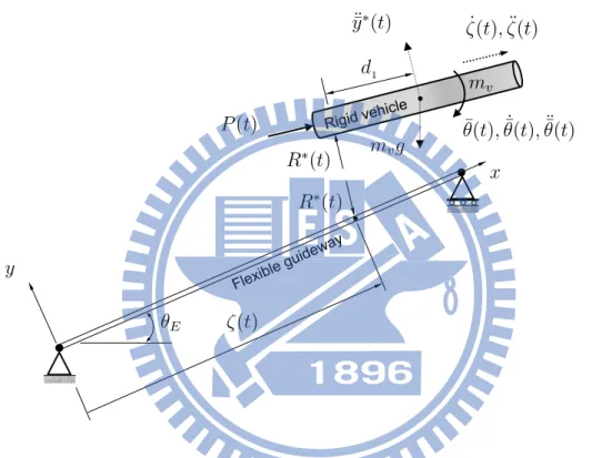
θE ζR d ζF P (t) mv, J d1 ζ(t), ˙ζ(t), ¨ζ(t) EI, ρA, c x y
Figure 3.1: A typical flexible guideway used for rigid vehicle launch.
During the motion of the vehicle, the two shoes of the vehicle are assumed to slide along the guideway by means of a rigid contact. The thrust vector is assumed
to be along the vehicle’s centerline (C.L.) and it always coincides with the line joining the two contact points. The vehicle and the guideway are considered to be two free bodies in Fig. 3.2. The typical displacement relationship between the vehicle and its guideway is shown in Fig. 3.3.
θE L ζ(t) d P (t) R(t) R(t) F (t) F (t) mvg d1 ¨ ¯ y(t) ˙ ζ(t), ¨ζ(t) x y
Figure 3.2: Free-body diagrams of a vehicle and its guideway.
yR(t) w(ζ, t) mvg w(ζ + d, t) C.L. ¯ y(t) ¯ θ(t) yF(t) x
3.1.1 Position history of vehicle
As mentioned in Chapter 2, two phases exist with the vehicle during take-off, i.e., the two-shoe contact phase and the tip-off phase. From the typical thrust-time curve shown in Fig. 2.3 and the design parameters of the vehicle and its guideway, one can easily find the position of the rear shoe, ζ(t) (see Fig. 3.2), tF and tR by using the
formulas for ζ(t), tF and tR given in Chapter 2.
3.1.2 Two-shoe contact phase
The vibration of the guideway is modeled as a simply supported Euler-Bernoulli beam with viscous damping and is subjected to given initial conditions and specified bound-ary conditions. Let F and R denote the moving loads of the contact points (see Fig. 3.2). Assume small deformations for beams, and the governing equation of transverse vibrations can be given by the following partial differential equation:
EI∂ 4w (x, t) ∂x4 + ρA ∂2w (x, t) ∂t2 + c ∂w(x, t) ∂t = Rδ (x, ζ) + F δ (x, ζ + d) (3.1)
where w (x, t) is the transverse displacement of the guideway; EI, the constant flexural rigidity of the guideway; ρA, the mass per unit length of the guideway; c, the damping coefficient per unit length; δ (.), the Dirac delta function; and Rδ (x, ζ) + F δ (x, ζ + d), an external force acting on the guideway because of the motion of the vehicle in the two shoe contact phase.
Based on the aforementioned assumptions and the relationship of geometry in Fig. 3.3, the transverse displacement ¯yof the vehicle can be expressed as
¯
y = d1
dyF +
(d− d1)
d yR (3.2)
where d denotes the distance between the shoes of the vehicle; d1 is the distance
and yF = w(ζ + d, t) denote the displacements of the two shoe contact points in the y-direction, respectively, when the vehicle is moving along the deformed guideway.
The pitch angle ¯θof vehicle can be obtained by
¯
θ = yF − yR
d (3.3)
Accordingly, the equations of motion of the vehicle can be written as
mvy =¨¯ −R − F + mvg cos θE (3.4)
J ¨θ = d¯ 1R− (d − d1)F (3.5)
where the overhead dot (·) denotes the differentiation with respect to time t; mv de-notes the mass of the vehicle; J is the mass moment of inertia of the vehicle; θE presents
the angle of inclination of the guideway; and g is the gravitational acceleration. Differentiation Eqs. (3.2) and (3.3) twice with respect to time t yields
¨ ¯ y = d1 dy¨F + (d− d1) d y¨R (3.6) ¨ ¯ θ = y¨F − ¨yR d (3.7)
Substituting ¨¯yfrom Eq. (3.6) into Eq. (3.4) results in
R + F =−mv [ d1 dy¨F + (d− d1) d y¨R ] + mvg cos θE (3.8)
Substituting ¨¯θ from Eq. (3.7) into Eq. (3.5) results in
R = 1 d1 [ J(¨yF − ¨yR) d + (d− d1)F ] (3.9)
Substituting R from Eq. (3.9) into Eq. (3.8), we have 1 d1 [ J(¨yF − ¨yR) d + (d− d1)F ] + F =−mv [ d1 d y¨F + (d− d1) d y¨R ] + mvg cos θE (3.10)
Solving for R and F in Eqs. (3.9) and (3.10), we obtain
F = mv(¯gr1 + J1y¨R− J2y¨F) (3.11a)
R = mv(¯gr2 − J3y¨R + J1y¨F) (3.11b)
where r1, r2, J1, J2, J3, and ¯gare constants defined as follows:
r1 = d1 d r2 = d− d1 d J1 = J mvd2 − r1r2 J2 = J mvd2 + r2 1 J3 = J mvd2 + r2 2 g = g cos θ¯ E (3.12)
The expressions (¨yR, ¨yF), (2 ˙y0Rζ, 2 ˙˙ y0 F
˙
ζ), and (yR00ζ˙2, y00
F
˙
ζ2) denote the acceleration
of the inertia force, Coriolis force, and centrifugal force, respectively, at the shoes, at the rear and front contact points; ˙ζ denotes the velocity of the moving vehicle in the local x-direction (see Fig. 3.2); the prime (0)denotes the differentiation with respect to coordinate x. Because yR = w(ζ, t) and yF = w(ζ + d, t), ˙yR0 =
∂2w(ζ,t) ∂x∂t , ˙yF0 = ∂2w(ζ+d,t) ∂x∂t , y00 R = ∂2w(ζ,t) ∂x2 and y00F = ∂2w(ζ+d,t) ∂x2 .
The equations of the contact load between the vehicle and its guideway are de-rived by taking into account the effects of the inertia force, Coriolis force, and cen-trifugal force of the moving vehicle. Equations (3.11a) and (3.11b) can be rewritten as follows:
R = mv [ ¯ gr2 − J3 ( ¨ yR + 2 ˙y 0 R ˙ ζ + yR00ζ˙2 ) + J1 ( ¨ yF + 2 ˙y 0 F ˙ ζ + yF00ζ˙2 )] (3.13a) F = mv [ ¯ gr1 + J1 ( ¨ yR + 2 ˙y 0 R ˙ ζ + y00Rζ˙2 ) − J2 ( ¨ yF + 2 ˙y 0 F ˙ ζ + yF00ζ˙2 )] (3.13b)
In order to obtain the approximate solution of the coupled system of equations, the transverse displacement of the guideway, w (x, t), can be expressed as the super-position of the normal mode, shown as follows:
w (x, t) =
N ∑
i=1
φi(x) Yi(t) ; 0≤ t ≤ tF (3.14)
where φi(x)denotes the ith mode of the guideway, satisfying the boundary conditions, and Yi(t)is the generalized coordinate corresponding to the ith mode. The modes of natural vibrations of a simply supported homogeneous beam can be easily found and are given as follows:
φi(x) = sin (βix) (3.15)
where β4
i = ω2i ·
ρA
EI, βiL = iπ; L is the length of the guideway; ωi is circular frequency
of the ith vibration of the guideway [38].
Substituting Eqs. (3.13), (3.14), and (3.15) into Eq. (3.1), multiplying both sides of the equation by φn(x), and integrating with respect to x from 0 to L, we obtain the following expression: ¨ Yi(t) + 2ξiωiY˙i(t) + ωi2Yi(t) = 2mv ρAL { ¯ gr2sin ( iπζ L ) − N ∑ j=1 ΦmijY¨j(t)− N ∑ j=1 ΦcijY˙j(t) − N ∑ j=1 ΦkijYj(t) + ¯gr1sin [ iπ (ζ + d) L ]} (3.16)
¨ Yi(t) + ρM N ∑ j=1 ΦmijY¨j(t) + 2ξiωiY˙i(t) + ρM N ∑ j=1 ΦcijY˙j(t) + ωi2Yi(t) + ρM N ∑ j=1 ΦkijYj(t) = Qi (3.17) where ρM = 2mv ρAL; ρF = 2mvg¯
ρAL; and Qi, Φmij, Φcij, and Φkij are expressed as follows:
Qi = ρF { r2sin ( iπζ L ) + r1sin [ iπ (ζ + d) L ]} (3.18) Φmij = { J3sin ( jπζ L ) − J1sin [ jπ (ζ + d) L ]} sin ( iπζ L ) − { J1sin ( jπζ L ) − J2sin [ jπ (ζ + d) L ]} sin [ iπ (ζ + d) L ] (3.19a) Φcij = 2jπ ˙ζ L { J3cos ( jπζ L ) − J1cos [ jπ (ζ + d) L ]} sin ( iπζ L ) − 2jπ ˙ζ L { J1cos ( jπζ L ) − J2cos [ jπ (ζ + d) L ]} sin [ iπ (ζ + d) L ] (3.19b) Φkij = ( jπ ˙ζ L )2{ − J3sin ( jπζ L ) + J1sin [ jπ (ζ + d) L ]} sin ( iπζ L ) + ( jπ ˙ζ L )2{ J1sin ( jπζ L ) − J2sin [ jπ (ζ + d) L ]} sin [ iπ (ζ + d) L ] (3.19c) wherei = 1, 2, ..., N and j = 1, 2, ..., N
Because the system is initially at rest, the guideway’s initial velocity and acceler-ation are zero. Hence, the initial conditions are ¨Yi(0) = 0, ˙Yi(0) = 0, ˙ζ = 0, and Φkij = 0. Application of these initial conditions leads to the initial displacement Yi(0) of the guideway because of the static load of the vehicle is
Yi(0) = ρF ω2 i { r2sin ( iπζR L ) + r1sin [ iπ (ζR + d) L ]} (3.20)
3.1.3 Tip-off phase
When the front shoe loses contact with the guideway, F reduces to zero in the tip-off phase. The vehicle and guideway can be considered as two free bodies shown in Fig. 3.4. ζ(t) θE y P (t) R∗(t) R∗(t) x mvg ¯ θ(t), ˙¯θ(t), ¨θ(t)¯ d1 mv ¨ ¯ y∗(t) ζ(t), ¨˙ ζ(t)
Figure 3.4: Free-body diagrams of vehicle in tip-off phase.
In the tip-off phase, Eq.(3.13b) equal to zero
F∗ = mv [ ¯ gr1 + J1 ( ¨ yR + 2 ˙y0 R ˙ ζ + y00 R ˙ ζ2 )∗ − J2 ( ¨ yF + 2 ˙y0 F ˙ ζ + y00 F ˙ ζ2 )∗] = 0 (3.21) Therefore, ( ¨ yF + 2 ˙y0 F ˙ ζ + y00 F ˙ ζ2 )∗ = 1 J2 [ ¯ gr1 + J1 ( ¨ yR + 2 ˙y0 R ˙ ζ + y00 R ˙ ζ2 )∗] (3.22)