A study of reduced support vector machines

A Study on Reduced Support Vector Machines

Kuan-Ming Lin and Chih-Jen Lin

Abstract—Recently the reduced support vector machine

(RSVM) was proposed as an alternate of the standard SVM. Motivated by resolving the difficulty on handling large data sets using SVM with nonlinear kernels, it preselects a subset of data as support vectors and solves a smaller optimization problem. However, several issues of its practical use have not been fully discussed yet. For example, we do not know if it possesses com-parable generalization ability as the standard SVM. In addition, we would like to see for how large problems RSVM outperforms SVM on training time. In this paper we show that the RSVM formulation is already in a form of linear SVM and discuss four RSVM implementations. Experiments indicate that in general the test accuracy of RSVM are a little lower than that of the standard SVM. In addition, for problems with up to tens of thousands of data, if the percentage of support vectors is not high, existing implementations for SVM is quite competitive on the training time. Thus, from this empirical study, RSVM will be mainly useful for either larger problems or those with many support vectors. Experiments in this paper also serve as comparisons of: 1) different implementations for linear SVM and 2) standard SVM using linear and quadratic cost functions.

Index Terms—Reduced support vector machine, support vector

machine.

I. INTRODUCTION

W

instance-label pairs ( , ), where and

, the support vector technique solves the following optimization problem:

(1) Since maps into a higher (maybe infinite) dimensional space, practically we solve its dual, a quadratic programming problem with the number of variables equal to

(2)

where is the vector of all ones, is an by

pos-itive semi-definite matrix, , and

is the kernel function.

Manuscript received March 1, 2002; revised November 25, 2002. This work was supported in part by the National Science Council of Taiwan under Grant NSC 90-2213-E-002-111.

The authors are with the Department of Computer Science and Information Engineering, National Taiwan University, Taipei 106, Taiwan, R.O.C. (e-mail: [email protected]).

Digital Object Identifier 10.1109/TNN.2003.820828

For large-scale problems, the difficulty of solving (2) results

from the fully dense matrix , which cannot be

saved in the main memory. Thus, traditional optimization algo-rithms like Newton or Quasi-Newton cannot be directly used. Currently one major method is the decomposition method (for example, [8], [18], [20]) which solves a sequence of smaller-sized problems so the memory difficulty is avoided. However, for huge problems with many support vectors, the decomposi-tion method still suffers from slow convergence. On the other

hand, if the linear kernel (i.e. ) is used, is

directly the product of a rectangular matrix and its transpose so we can exploit more possibilities to design efficient algorithms. Thus, here we mainly consider the more difficult case by using nonlinear kernels.

Recently [10] proposed to restrict the number of support vec-tors by solving the reduced support vector machines (RSVM). The main characteristic of this method is to reduce the matrix from to , where is the size of a randomly selected subset of training data considered as candidates of support vec-tors. The smaller matrix can be stored in memory, so optimiza-tion algorithms such as Newton method can be applied. RSVM is different from directly solving smaller SVM problems with a subset of training data because the constraints in the primal problem (1) are still kept during the optimization process. In [10], the authors showed the performance (testing accuracy) is as good as the regular SVM. As RSVM essentially uses less information than the regular SVM, we feel there is a need to conduct some serious comparisons. This is the first aim of the paper. Our experiments show that in general the testing accu-racy of RSVM is a little lower than SVM.

Moreover, as the training efficiency is the main motivation of RSVM, we would like to discuss its different implementations, and compare their training time with the regular SVM. In ad-dition, we investigate for how large problems, RSVM becomes an efficient alternate of SVM. Results show that for problems with up to tens of thousands of data, if the percentage of sup-port vectors is not high, existing implementations for SVM are quite competitive on the training time. Thus, from this empirical study, RSVM will be mainly useful for either larger problems or those with many support vectors. We note that results here are mainly empirical and we do not conduct further theoretical analysis about the generalization error.

This paper is organized as follows. In Section II, we outline the key modifications from standard SVM to RSVM. In Sec-tion III, we detail the smooth SVM (SSVM) method used in [11], and apply three more techniques, the least square SVM (LS-SVM) [23], the Lagrangian SVM (LSVM) [15], and the decomposition method to solve the RSVM problem. Issues re-lated to practical implementations such as stopping criteria and approaches for solving multiclass problems are in Section IV.

Numerical experiments are in Section V which present that the accuracy of RSVM is usually lower than that of SVM. We also discuss that different techniques for solving RSVM have some minor differences on the accuracy, but using LS-SVM method is the fastest on training. In Section VII, there is an attempt to make modifications on the original RSVM formulation. Finally we have some discussions and conclusions in Section VIII.

II. REDUCEDSUPPORTVECTORMACHINEFORMULATION

Here, we outline the key modifications from standard SVM to RSVM in [10]. They start from adding an additional term to the objective function of (1)

(3) (4) Its dual form becomes a simpler bound-constrained problem

(5) The approach of adding and then obtaining a bounded dual was proposed in [4] and [14]. This is equivalent to adding a constant feature to the training data and finding a separating hyperplane passing through the origin. Numerical experiments in [7] show that the accuracy does not vary much when is added.

It is known that, at the optimal solution, is a linear combi-nation of training data:

(6)

If we substitute into (3), using

(7)

(8)

we obtain a new optimization problem

(9) Though (9) is different from (5), the dual problem, we can show that for any optimal of (9), the corresponding defined by (6) is also an optimal solution of (3), so we can solve (9)

instead of (5). We put the details in Appendix A. The reformu-lation of (3) to (9) was first used in [19].

The idea of RSVM is to reduce the number of support vectors. It is achieved by randomly selecting a subset of samples for constructing

(10)

where contains indices of this subset. By substituting (10) into (4), we can get a similar problem as (9), with the number of major variables (i.e. ) reduced to :

(11) where is the collection of all , . Note that now is the size of . We use to represent the submatrix of columns corresponding to . Thus, there are still constraints. Following the generalized SVM by Mangasarian [10], [13] simplified the

term to so RSVM solves

(12) Later on we will address more about this simplification. Note that throughout the discussion we omit writing the constraint

as it is always satisfied at the optimal solution.

The idea of using (10) is similar to the Radial Basis Func-tion (RBF) networks [17] which either select a subset of training data or generate some “centers” in order to construct a decision function. The RBF networks directly start from a form similar to (10) and the regularization term used is . If the inequality (12) is replaced by an equality, (12) is in a form of the RBF net-works. There are already comparisons between SVM and RBF networks. For example, [22] shows that SVM performs better as the RBF networks use less information. Therefore, we are curious whether similar scenarios apply to SVM and RSVM, which will be one of the main aims of this paper.

III. DIFFERENTIMPLEMENTATIONS FORRSVM In [10], the authors solved RSVM by SSVM, which basi-cally approximates the original problem by an unconstrained one. However, we observe that (12) is already in the primal form of the original linear SVM. Therefore, existing methods which focus on solving linear SVM can be applied here. To see this,

suppose contains indices , in the following we

point out the relation between (3) and (12):

Therefore, if we consider ,

as the training data, then the number of attributes is and ( , ) are coefficients of the separating hyperplane. In other words,

it is like that we are training a linear SVM with data. For linear SVM the number of features is usually much smaller than the number of data so there are methods which take this prop-erty. However, for nonlinear SVM where the dimensionality of the feature space is large, such methods may not be applicable. Thus, usually the dual problem is considered instead. Now we choose so we are safe to apply methods which were originally mainly suitable for linear SVM.

In Section III-A we will discuss the SSVM originally used in [10] while in Sections III-B–III-D, we consider three methods which were suitable for linear SVM: Least Square SVM (LS-SVM) [23], Lagrangian SVM (LSVM) [15], and the decomposition method for linear SVM.

Before describing different implementations, for the sake of convenience, with the following substitution:

we consider a simpler form

(13)

A. Using SSVM

By defining and applying the property that

whenever , the th constraint (13) must be active, the con-strained problem (13) can be transformed to the unconcon-strained one

(14)

If the objective function is differentiable (or twice differ-entiable), we can use general methods (for example, Newton method, quasi-Newton method, etc.) to find an optimal solu-tion. Unfortunately is not differentiable so SSVM approximates the function by

where is called the smoothing parameter. When approaches

to infinity, converges to .

We observe that if is large, sometimes huge objective values of (14) may cause numerical difficulties. For example, if a method for solving (14) uses the absolute difference on objective values of two successive iterations as the stopping criterion, the large objective values may cause very long iterations before reaching a specified tolerance. Hence, we divide the objective function by

(15)

We solve (15) by a Newton’s method implemented in the soft-ware TRON [12], which uses both the information of the first derivative (gradient) and the second derivative (Hessian).

While [10] did not give the explicit form of the gradient and the Hessian, we list them here as a reference. By defining

then

(16)

(17) where is a diagonal matrix with elements of on the diagonal. Details on deriving them can be found in Appendix A. TRON was originally designed for large sparse problems. Now the Hessian is dense so we use the modification in [7] to solve (15). As a Newton’s method is used, TRON possesses the property of quadratic convergence.

Time complexity analysis: Now the Hessian is by so the Newton’s method takes operations in each iteration for inverting or factorizing the Hessian. However, in order to obtain the Hessian, in (17), we need more operations: . Hence is the complexity of each iteration.

B. Using Least-Square SVM

Least-square SVM (LS-SVM), first introduced in [23], can solve linear SVM efficiently. It changes the inequality constraints to equalities, and solve the resulting linear system. Taking (3) as an example, they change the primal inequalities

(4) to and remove constraints

. Thus, substituting into the objective function we get an unconstrained problem:

(18) Of course, changing inequalities into equalities may affect the meaning of separating hyperplanes though this is not the topic we would like to discuss here.

For linear SVM (i.e. instead of is used), we can solve (18) directly by a linear system of variables where is the number of attributes as well as the length of . For nonlinear

SVM where , we must substitute into

(18) and solve a linear system with variables and . Thus, when is large, the same problem of conventional SVM for-mulations occurs: the matrix cannot be placed in the main memory, so it is not easy to solve a large dense linear system. As a result, LS-SVM so far is more suitable for linear SVM prob-lems.

Following the same procedure, here we change the inequality (13) to an equality:

and substitute into (13). Similar to the case of SSVM, we divide the objective function by and get an unconstrained problem where is the only variable

(20) With

we minimize by finding the solution of ,

(21) a positive definite linear system of size . As , (21) is small enough. Thus, we can use direct methods such as Gaussian elimination or Cholesky factorization to efficiently solve it.

Time complexity analysis: The cost of Gaussian elimination, , is less than that for computing the matrix multiplication which costs . Hence the total time complexity is

.

C. Using Lagrangian SVM

Here, we discuss Lagrangian SVM (LSVM) [15], another technique to solve SVM problems. LSVM is an iterative algo-rithm which solves the dual form (5). Define

. Then the Karush–Kuhn–Tucker (KKT) optimality condi-tions of (5) are

Again, we denote max ( , 0) by . The authors of [15] used the following identity between any two vector and :

(22) so the optimality conditions are equivalent to

(23) Thus, an optimal is a solution of the fixed-point equation and they applied the following iterative scheme:

(24) [15] showed that LSVM algorithm is linearly convergent if is chosen so that

Though in each iteration, we must invert the dense matrix , for linear SVM’s, the Sherman-Morrison-Woodbury (SMW) identity can be used. But it cannot be applied to nonlinear ker-nels where the input vectors are mapped into high (maybe in-finite) dimensional spaces. Thus, LSVM method so far is not practical for large-scale problems using nonlinear kernels. An

earlier comparison with LIBSVM, a decomposition method for standard SVM, is in [5], which shows that LSVM is slower when using nonlinear kernels.

We have mentioned earlier that RSVM is equivalent to a linear SVM problem, so the Lagrangian SVM algorithm can be used here. First, we write down the dual form of (13)

(25) Let

Lagrangian SVM solves

Here, is calculated using the SMW identity

In order to get , now the primal variable, we apply the rela-tionship (6):

Time complexity analysis: The generation and then

inver-sion of the matrix costs , where

the main task is the matrix multiplication. This can be done be-fore all iterations. Then in each iteration, the main cost is several matrix-vector multiplications which costs operations. So

the total time complexity is .

Compared with SSVM, LSVM method seems need more itera-tions since it guarantees only linear convergence.

D. Using Decomposition Methods for Linear SVM

Originally the decomposition method [8], [18], [20] was pro-posed to handle the nonlinear SVM whose kernel matrix is fully dense and cannot be stored. It is an iterative process where in each iteration the index set of variables is separated to two sets and , where is the working set. Then in that iteration variables corresponding to are fixed while a subproblem on variables corresponding to is minimized.

If is the size of the working set and further tech-niques such as caching and shrinking are not used, in each it-eration columns of the kernel matrix are used for calculating , where is the kernel matrix and is a vector with at most nonzero modifications in one iteration. Therefore, the total complexity is

where is the number of attributes and we assume each kernel evaluation costs . However, for linear SVM, is in a form

of and , an matrix, contains all training data. Thus

(26)

costs only operations.

Therefore, for large problems where caching recently used is not very useful, in each iteration, using (26) can be times faster than the regular decomposition method. This trick has

been implemented in, for example, [8] and BSVM

(version 2.03 and later) [7]. Of course the selection of becomes an issue. It should be larger than the one used for nonlinear SVM but also cannot be too large. Otherwise solving the subproblem which has variables may cost more than for (26).

For RSVM, since , we consider RSVM as a linear

SVM and apply a decomposition method to solve its dual. However, we consider the formulation with linear cost function

so instead of (25), the dual problem is

(27) The reason is that we will use the software BSVM which solves (27) but not (25).

In the following, we summarize the time complexity of the four approaches discussed earlier, see the table at the bottom of page.

IV. IMPLEMENTATIONISSUES A. Stopping Criteria

In order to compare the performance of different methods, we should use comparable stopping criteria for them. However, so many differences among these methods prohibit us from finding precisely equivalent stopping criteria for all methods. Still, we try to use reasonable criteria which will be described below in detail.

In the next section we will use LIBSVM as the representative for solving the regular nonlinear SVM so we first explain its stopping criterion. LIBSVM is a decomposition method which solves the dual form of the standard SVM with a linear cost function:

(28)

It is shown in [3] that if , the KKT condition of (28) is equivalent to

(29) For practical implementations, a stopping tolerance is set, and the stopping criterion can be

(30)

where we choose .

To check the performance of using linear and quadratic cost functions, we also modify LIBSVM to solve (2). It is easy to see that a similar stopping criterion can be used. Another decompo-sition software BSVM is used for solving RSVM as described in Section III-D. It also has a similar stopping criterion.

The LSVM method, another implementation for RSVM, solves problems in the dual form (25), hence a stopping criteria can be similar. Now

The KKT condition of (25) shows that if and

then is an optimal solution. Note that during LSVM iterations, the constraints are not maintained. Thus, we consider a stopping criterion as follows:

and

(31)

We also set here.

For the SSVM, we simply employ the original stopping cri-terion of TRON:

(32) where is defined in (15), is the initial solution, and

.

Note, that for LS-SVM implementation, we use direct methods to solve the linear system, therefore no stopping criterion is needed.

B. Multiclass RSVM

Although SVM was originally designed for binary classifi-cation, several methods have been proposed to solve multiclass classification. A common way is by considering a set of binary

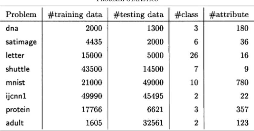
TABLE I PROBLEMSTATISTICS

SVM problems, while some authors also proposed methods that consider all classes at once. These methods in general can also be applied to RSVM.

There have been some comparisons of methods for multiclass SVM. In [6] we compare different decomposition implementa-tions, and in [24] some comparisons of methods for multiclass LS-SVM are given. They both indicate that the one-against-one method performs well in practice. So we use it for our imple-mentation here. Suppose there are classes of data. This method constructs classifiers where each one trains data from two classes. In classification we use a voting strategy: each bi-nary classification is considered to be a voting where votes can be cast for all data points —in the end point is designated to be in a class with maximum number of votes.

The implementation of all methods mentioned above is avail-able at http://www.csie.ntu.edu.tw/~cjlin/libsvm/libsvmtools.

V. EXPERIMENTS

In this section we conduct experiments on some commonly used problems. We choose large multiclass datasets from the Statlog collection: dna, satimage, letter, and shuttle [16]. We also consider mnist [9], an important benchmark for handwritten digit recognition. The problem ijcnn1 is from the first problem of IJCNN challenge 2001 [21]. Note, that we use the winner’s transformation of raw data [2]. Problem protein, is a data set for protein secondary structure prediction [26]. Finally, the problem adult, from the UCI “adult” data set [1] and compiled by Platt [20], is also included. For the adult dataset, there are several real-izations. Here, we only consider the realization with the smallest training set; the full dataset with training data (including du-plicated ones) removed is taken as the test set. We choose this dataset because it has been tested in the RSVM paper [10]. Our preparation of the training and test sets is also similar to theirs. Except problems dna, ijcnn1, protein, and adult whose data values are either binary or already in a small range, we linearly scale all training data to be in [ 1, 1]. Then test data, available for all problems, are scaled accordingly. Note that for problem mnist, it takes too much training time if the whole 60 000 training samples are used, so we consider the training and testing data together (i.e. 70 000 samples) and then cut the first 30% for training and test the remaining 70%. Also, note that for the problem satimage, there is one missing class. That is, in the original application there is one more class but in the

data set no examples are with this class. We give problem statis-tics in Table I. Some problems with a large number of attributes may be very sparse. For example, for each instance of protein, only 17 of the 357 attributes are nonzero.

We compare four implementations of RSVM discussed in Section III with two implementations of the regular SVM: linear and quadratic cost functions [(28) and (2)]. For reg-ular SVM with the linear cost function, we use the software LIBSVM which implements a simple decomposition method. We can easily modify LIBSVM to solve the formulation with a quadratic cost function, which we will refer to as LIBSVM-q in the rest of this paper. However, we will not use it for solving RSVM as LIBSVM implements an SMO type algorithm where the size of the working set is restricted to two. In Section III-D we have shown that larger working sets should be used when applying decomposition methods to linear SVM.

The computational experiments for this section were done on a Pentium III-1000 with 1024 MB RAM using the gcc com-piler. For three of the four RSVM methods (SSVM, LS-SVM, and LSVM), the main computational work is some basic ma-trix operations so we use ATLAS to optimize the performance [27]. This is very crucial as otherwise a direct implementation of these matrix operations can at least double or triple the compu-tational time. For decomposition methods where the kernel ma-trix cannot be fully stored we allocate 500 MB memory as the cache for storing recently used kernel elements. Furthermore, LIBSVM, LIBSVM-q, and BSVM all use a shrinking technique so if most variables are finally at bounds, they solve smaller problems by considering only free variables. The details on the shrinking technique are in [3, Section 4].

Next, we discuss the selection of parameters in different im-plementations. It is of course a tricky issue on selecting , the size of the subset of RSVM. This depends on practical situations such as how large the problem is. Here in most cases we fix to be 10% of the training data, which was also considered in [10]. For multiclass problems, we cannot use the same for all bi-nary problems as the data set may be highly unbalanced. Hence we choose to be 10% of the size of each binary problem so a smaller binary problem use a smaller . In addition, for prob-lems shuttle, ijcnn1, and protein, binary probprob-lems may be too large for training. Thus, we set for these large binary problems. This is similar to how [10] deals with large problems. Once the size is determined, for all four implementations, we se-lect the same subset for each binary RSVM problem.

TABLE II

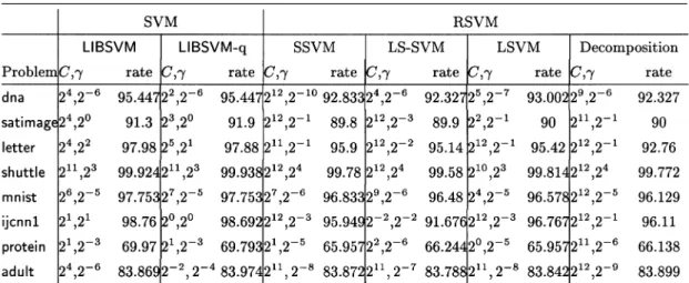
A COMPARISON ONTESTINGACCURACY

We need to decide some additional parameters prior to exper-iments. For SSVM method, the smoothing parameter is set to 5 because the performance is almost the same for . For

LSVM method, we set which is the same as that

in [15]. We do not conduct cross validation for selecting them as otherwise there are too many parameters. For BSVM which is used to solve linear SVM arising from RSVM, we use all de-fault settings. In particular, the size of the working set is 10.

The most important criterion for evaluating the performance of these methods is their accuracy rate. However, it is unfair to use only one parameter set and then compare these methods. Practically for any method we have to find the best parameters by performing the model selection. This is conducted on the training data where the test data are assumed unknown. Then the best parameter set is used for constructing the model for future testing. To reduce the search space of parameter sets, here

we consider only the RBF kernel , so

the parameters left for decision are kernel parameter and cost parameter . In addition, for multiclass problems we consider

that and of all binary problems via the

one-against-one approach are the same.

For each problem, we estimate the generalized

ac-curacy using different and

. Therefore, for each problem we

try combinations. For each pair of ( , ),

the validation performance is measured by training 70% of the training set and testing the other 30% of the training set. Then we train the whole training set using the pair of ( , ) that achieves the best validation rate and predict the test set. The resulting accuracy is presented in the “rate” columns of Table II. Note that if several ( , ) have the same accuracy in the validation stage, we apply all of them to the test data and report the highest rate. If there are several parameters that achieve the same highest testing rate, we report the one with the minimal training time.

VI. RESULTS A. Accuracy

Table II shows the result of comparing LIBSVM, LIBSVM-q, and the four RSVM implementations. We present the optimal

parameters ( , ) and the corresponding accuracy rates. It can be seen that optimal parameters ( , ) are in various ranges for different implementations so it is essential to test so many pa-rameter sets. We observe that LIBSVM and LIBSVM-q have very similar accuracy. This does not contradict the current un-derstanding in this area as we have not seen any report which shows one has higher accuracy than the other. Except ijcnn1, the difference of the four RSVM implementations is also small. This is reasonable as essentially they solve (12) with minor mod-ifications.

For all problems, LIBSVM and LIBSVM-q perform better than RSVM implementations. We can expect this because for RSVM the support vectors are randomly chosen in advance, therefore we cannot ensure that the support vectors are impor-tant representatives of the training data. This seems imply that if problems are not too large, we would like to stick on the original SVM formulation. We think this situation is like the comparison between RBF networks and SVM [22] since RBF networks se-lect only several centers, it may not extract enough information. In general the optimal of RSVM is much larger than that of the regular SVM. As RSVM is indeed a linear SVM with a lot more data than the number of attributes, it tends to need a larger so that data can be correctly separated. How this property affects its model selection remains to be investigated.

We also observe that the accuracy of LS-SVM is a little lower than SSVM and LSVM. In particular, for problem ijcnn1 the dif-ference is quite large. Note that ijcnn1 is an unbalanced problem where 90% of the data have the same label. Thus, the 91.7% ac-curacy by LS-SVM is quite poor. We suspect that the change of inequalities to equalities for LS-SVM may not be suitable for some problems.

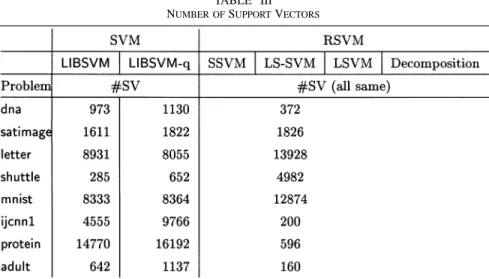
B. Number of Support Vectors

In Table III we report the number of “unique” support vectors for each method. We say “unique” support vectors because for the one-against-one approach, one training data may be a sup-port vector of different binary classifiers. Hence, we resup-port only the number of training data which corresponds to at least one support vector of a binary problem. Note that as we specified, all three RSVM implementations have the same number of sup-port vectors.

TABLE III NUMBER OFSUPPORTVECTORS

TABLE IV

TRAININGTIME ANDTESTINGTIME(INSECONDS)

For letter, shuttle and mnist the RSVM approach has a large number of support vectors. A reason is that subsets selected for all binary problems are quite different. This is unlike standard SVM where important vectors may appear in different binary problems so the number of unique support vectors is not that large. An alternative way for RSVM may be to select a subset of all data first and then for each binary problem support vec-tors are elements in this subset which belong to the two corre-sponding classes. This will reduce the testing time as [6] has discussed that if the number of classes is not huge, it is propor-tional to the number of unique support vectors. On the contrary, training time will not be affected much as the size of binary problems is still similar.

Though the best parameters are different, roughly we can see LIBSVM-q requires more support vectors than LIBSVM. This is consistent with the common understanding that the quadratic cost function leads to more data with small nonzero ’s. For protein LIBSVM and LIBSVM-q both require many training data as support vectors. Indeed most of them are “free” support vectors (i.e. corresponding dual variables not at the upper bound). Such cases are very difficult for decomposition methods and their training time will be discussed in the next subsection.

C. Training and Testing Time

We report the training time and testing time in Table IV. For the four RSVM implementations, we find their testing time is quite close so we post only that of the LSVM implementation. Note that here we report only the time or solving the optimal model. Except the LS-SVM implementation for RSVM which solves a linear equation for each parameter set, the training time of all other approaches depends on parameters. In other words, their number of iterations may vary for different param-eter sets. Thus, results here cannot directly imply which method is faster as the total training time depends on the model selection strategy. However, generally we can see for problems with up to tens of thousands of data, the decomposition method for the traditional SVM is still competitive. Therefore, RSVM will be mainly useful for larger problems. In addition, RSVM possesses more advantages on solving large binary problems because for multiclass data sets we can afford to use decomposition methods to solve several smaller binary problems.

Table IV also indicates that the training time of decomposi-tion methods for SVM strongly depends on the number of sup-port vectors. For the problem ijcnn1, compared to the standard LIBSVM, the number of support vectors using LIBSVM-q is

TABLE V

TESTINGACCURACY: A COMPARISON ONSOLVING(21)AND(34)

doubled and then the training time is a lot more. This has been known in the literature as starting from the zero vector as the initial solution, the smaller the number of support vectors (i.e. nonzero elements at an optimal solution) is, the fewer variables may need to be updated in the decomposition iterations. As dis-cussed earlier, protein is a very challenging case for LIBSVM and LIBSVM-q due to the high percentage of training data as support vectors. For such problem RSVM is a promising alter-nate: Using very few data as support vectors, the computational time is largely reduced and the accuracy does not suffer much.

Among the four RSVM implementations, the LS-SVM method is the fastest in the training stage. This is obvious as its cost is just that of one iteration of the SSVM method. Therefore, from the training time of both implementations we can roughly see the number of iterations of the SSVM method. As expected, the Newton’s method converges quickly, usually in less than 10 iterations. On the other hand, LSVM which is cheaper for each iteration, needs hundreds of iterations. For quite a few problems it is the slowest.

It is interesting to see that the decomposition method, not originally designed for linear SVM, performs well on some problems. However, it is not very stable as for some difficult cases, the number of training iterations is prohibitive.

VII. MODIFICATIONS ON THERSVM FORMULATION

Remember we mentioned in Section II that following the

generalized SVM the authors of [10] replace in

(11) by in (12). So far we only see that for the LSVM implementation, if without doing so we may have troubles to obtain and use the dual problem. For SSVM and LS-SVM, can be kept and the same methods can still be applied. As the change leads to the loss of the property on maximizing the margin, we are interested in whether the performance (testing accuracy) is sacrificed or not.

Without changing the term in (20), LS-SVM

formulation is

(33) Thus, we will solve a different linear system

(34) Though (34) is nearly the same as (21), it is only a positive semi-definite but not positive semi-definite system. Thus, LU factorization

instead of Cholesky factorization is used. This change affects very little to the training time according to the time complexity analysis in Section III-B. A comparison on the testing accuracy between solving (21) and (34) is in Table V. We can see that their accuracy is very similar. Therefore, we conclude that the use of a simpler quadratic term in RSVM is basically fine.

VIII. DISCUSSIONS ANDCONCLUSIONS

We have discussed four multiclass implementations for the RSVM formulations and have compared them with two decom-position methods based on LIBSVM. Experiments indicate that in general the test accuracy of RSVM is a little worse than that of the standard SVM. Though RSVM keeps similar constraints to the primal form of SVM, restricting support vectors from a randomly selected subset still downgrades the performance. For the training time which is the main motivation of RSVM we show that based on the current implementation techniques, RSVM will be faster than the regular SVM on large problems or some difficult cases with many support vectors. Therefore, for median-sized problems, standard SVM should be used but for large problems, as RSVM can effectively restrict the number of support vectors, it can be an appealing alternate. Regarding the implementation of RSVM, least-square SVM (LS-SVM) is the fastest among the four methods compared here though its accuracy is a little lower. Thus, for very large problems it is ap-propriate to try this implementation first.

APPENDIX A

RELATIONBETWEEN(9)AND(3)

The derivation from (7) and (8) to (9) shows only that if ( , , ) and are primal and dual optimal solutions, respec-tively, then ( , , ) is feasible for (9). Hence, before using (9) in practice we want to make sure that any optimal ( , , ) of (9) can construct an optimal for the primal problem (3).

It is easy to see this. By using , ( , ,

) is feasible for (3). Since we have shown that ( , , ) is feasible for (9)

Thus, ( , , ) is optimal for the primal. APPENDIX B

DERIVATIONS OF(16)AND(17)

In order to simplify the complex term, we define the vector

and then

(36) The differentiations of and are

Finally we obtain the gradient and Hessian of :

where is defined as

if if

If we define . ._. for vector with

dimension , we obtain a more clear matrix form

ACKNOWLEDGMENT

The authors thank M. Heiler, Y.-J. Lee, and X.-F. Lu for many helpful comments.

REFERENCES

[1] C. L. Blake and C. J. Merz, “UCI Repository of Machine Learning Databases, Tech. Rep.,” Univ. California, Dept. Information and Com-puter Science, Irvine, CA, 1998.

[2] C.-C. Chang and C.-J. Lin, “IJCNN 2001 challenge: generalization ability and text decoding,” in Proc. IJCNN, 2001.

[3] LIBSVM: A Library for Support Vector Machines, C.-C. Chang and C.-J. Lin. (2001). http://www.csie.ntu.edu.tw/~cjlin/libsvm [Online] [4] T.-T. Friess, N. Cristianini, and C. Campbell, “The kernel adatron

algo-rithm: a fast and simple learning procedure for support vector machines,” in Proc. 15th Int. Conf. Machine Learning, 1998.

[5] M. Heiler, “Optimization criteria and learning algorithms for large margin classifiers,” Master’s thesis, Univ. Mannheim Germany, Dept. Mathematics and Computer Science, Computer Vision, Graphics, and Pattern Recognition Group, Mannheim, Germany, 2001.

[6] C.-W. Hsu and C.-J. Lin, “A comparison of methods for multiclass support vector machines,” IEEE Trans. Neural Networks, vol. 13, pp. 415–425, 2002.

[7] , “A simple decomposition method for support vector machines,” Machine Learning, vol. 46, pp. 291–314, 2002.

[8] T. Joachims, “Making large-scale SVM learning practical,” in Advances in Kernel Methods—Support Vector Learning, A. J. Smola, C. J. C. Burges, and B. Schölkopf, Eds. Cambridge, MA: MIT Press, 1998. [9] Y. LeCun. MNIST Database of Handwritten Digits. [Online] Available:

http://yann.lecun.com/exdb/mnist/

[10] Y.-J. Lee and O. L. Mangasarian, “RSVM: reduced support vector ma-chines,” in Proc. 1st SIAM Int. Conf. Data Mining, 2001.

[11] , “SSVM: a smooth support vector machine for classification,” Computational Optimization and Applications, vol. 20, no. 1, pp. 5–22, 2001.

[12] C. J. Lin and J. J. More, “Newton’s method for large-scale bound con-strained problems,” SIAM J. Optimization, vol. 9, pp. 1100–1127, 1999. [13] O. L. Mangasarian, “Generalized support vector machines,” in Advances in Large Margin Classifiers, D. Schuurmans, P. Bartlett, and B. S. A. J. Smola, Eds. Cambridge, MA: MIT Press, 2000, pp. 135–146. [14] O. L. Mangasarian and D. R. Musicant, “Successive overrelaxation for

support vector machines,” IEEE Trans. Neural Networks, vol. 10, pp. 1032–1037, Sept. 1999.

[15] , “Lagrangian support vector machines,” J. Machine Learning Res., vol. 1, pp. 161–177, 2001.

[16] D. Michie, D. J. Spiegelhalter, and C. C. Taylor, Machine Learning, Neural and Statistical Classification. Englewood Cliffs, N.J: Prentice-Hall, 1994.

[17] M. Orr, “Introduction to Radial Basis Function Networks,” Institute for Adaptive and Neural Computation, Edinburgh Univ., 1996.

[18] E. Osuna, R. Freund, and F. Girosi, “Training support vector machines: an application to face detection,” in Proc. IEEE CVPR’97, New York, 1997, pp. 130–136.

[19] E. Osuna and F. Girosi, “Reducing the run-time complexity of support vector machines,” in Proc. Int. Conf. Pattern Recognition, 1998. [20] J. C. Platt, “Fast training of support vector machines using sequential

minimal optimization,” in Advances in Kernel Methods—Support Vector Learning, A. J. Smola, C. J. C. Burges, and B. Schölkopf, Eds. Cambridge, MA: MIT Press, 1998.

[21] D. Prokhorov. IJCNN 2001 neural network competition. presented at Slide Presentation in IJCNN’01. [Online] http://www.geoci-ties.com/ijcnn/nncijcnn01.pdf

[22] B. Schölkopf, K.-K. Sung, C. J. C. Burges, F. Girosi, P. Niyogi, T. Poggio, and V. Vapnik, “Comparing support vector machines with gaussian kernels to radial basis function classiers,” IEEE Trans. Signal Processing, vol. 45, pp. 2758–2765, Nov. 1997.

[23] J. Suykens and J. Vandewalle, “Least square support vector machine classifiers,” Neural Processing Lett., vol. 9, no. 3, pp. 293–300, 1999. [24] , “Multiclass LS-SVMs: moderated outputs and coding-decoding

schemes,” in Proc. IJCNN, Washington, DC, 1999.

[25] V. Vapnik, The Nature of Statistical Learning Theory. New York: Springer-Verlag, 1995.

[26] J. Y. Wang, “Application of support vector machines in bioinformatics,” Master’s thesis, Dept. Computer Sci. Info. Eng., National Taiwan Uni-versity, 2002.

[27] R. C. Whaley, A. Petitet, and J. J. Dongarra, “Automatically Tuned Linear Algebra Software and the ATLAS Project,” Dept. Computer Sciences, Univ. Tennessee, 2000.

Kuan-Ming Lin received the B.S. degree in

computer science & information engineering, the B.S. degree in mathematics, and the M.S. degree in computer science & information engineering from National Taiwan University, Taiwan, R.O.C., in 2000 and 2002, respectively.

His research interests include machine learning, numerical optimization, and algorithm analysis.

Chih-Jen Lin (S’91–M’98) received the B.S. degree

in mathematics from National Taiwan University, Taiwan, R.O.C., in 1993 and the M.S. and Ph.D. degrees from the Department of Industrial and Operations Engineering, University of Michigan, Ann Arbor, in 1995 and 1998, respectively.

He is currently an Associate Professor in the De-partment of Computer Science and Information En-gineering, National Taiwan University. His research interests include machine learning, numerical opti-mization, and applications of operations research.