積極式可視度取樣法

Aggressive Visibility Computation using Importance

Sampling

Student: Ying-I Chiu

Advisor: Dr. Jung-Hong Chuang

Dr. Wen-Chieh Lin

Institute of Multimedia Engineering

College of Computer Science

National Chiao Tung University

ABSTRACT

We present an aggressive region-based visibility sampling algorithm for general 3D scenes. Our algorithm exploits the depth and color information of samples in the image space to construct an importance function that represents the reliability of the potentially visible set (PVS) of a view cell boundary, and places samples at the optimal positions according to the importance function. The importance function indicates and guides visibility samples to depth discontinuities of the scene such that more visible objects can be sampled to reduce the visual errors. The color information can help judge whether the visual errors are significant or not. Our experiments show that our sampling approach can effectively improve the PVS accuracy and computational speed compared to the adaptive approach proposed in [NB04] and the object-based approach in [WWZ+_06].

I would like to thank my advisors, Professor Jung-Hong Chuang and Wen-Chieh Lin, for their guidance, inspirations, and encouragement. I am also grateful to my senior colleague, Tan-Chi Ho, for his advices and suggestions on my thesis research. And then I want to express my gratitude to all my colleagues in CGGM lab: Jau-An Yang and Ta-En Chen discuss with me on research issues and helps me figure out the questions, Chien-Kai Lo and Yun Chien give me necessary information, Chia-Ming Liu and Yu-Chen Wu discuss about programming issues with me, Tsung-Shian Huang help me understand much rendering knowledge, and all my junior colleagues’ kind assistances, especially Shao-Ti Li for the implementation of comparison methods. I would like to thank Yong-Chen Chen in International Games System CO., LTD for kindly help. Lastly, I would like to thank my parents for their love, and support. Without their love, I could not pass all the frustrations and pain in my life.

Contents

1 Introduction 1

1.1 Contribution . . . 3 1.2 Organization of the thesis . . . 3

2 Related Work 5

2.1 Point-based Visibility . . . 5 2.2 Region-based Visibility . . . 7

3 Visibility Importance Sampling 13

3.1 Visibility Cube . . . 14 3.2 Sample Importance Function . . . 16 3.3 Visibility Importance Function . . . 18

4 Visibility Computation Framework 22

4.1 Hierarchical Space Partition and View Cells . . . 24 4.2 Visibility Sampling . . . 24 4.3 Computing Importance Function . . . 25

5 Results 26

5.1 Performance Comparison . . . 27 5.2 Image Error and PVS Accuracy . . . 31

6.1 Summary . . . 44 6.2 Limitations and Future Work . . . 45

Bibliography 46

List of Figures

1.1 A complex urban scene. Left: Only a small part of the scene (colored part) is visible if the viewer is on the road (the green area). Right: The visible set of the scene. [LSCO03] . . . 2 2.1 Hierarchical Occlusion Maps. [ZMHH97] . . . 6 2.2 Types of visibility. . . 8 2.3 Left: Visibility cubes. Right: Visibility cubes on the view cell boundaries. [NB04] 9 2.4 Left: Uniform sampling. Right: Adaptive sampling. [NB04] . . . 9 2.5 Left: The subdivision plane (green). Right: New samples added on the

subdi-vision plane. [NB04] . . . 9 2.6 Adaptive border sampling. [WWZ+06] . . . 10 2.7 Reverse sampling. [WWZ+06] . . . 11 2.8 Adaptive global visibility sampling (AGVS). The contribution of a ray can

af-fect multiple view cells. [BMW+09] . . . 12 3.1 The flow chart of computing the PVSs of a view cell boundary. . . 15 3.2 Left: Visibility cube samples on boundary faces of a view cell. There are 4

visibility samples on each boundary face in this case. Right: Each sample has a hemi-cube consisted of 5 images. Every polygon has an unique color in order to be recognized when gathering visible set. . . 17

gap facing the lower-right direction, so the viewpoint should move toward the right direction in order to see larger area in the gap. Right: The direction of the two gaps are opposite. After combining the contribution of two gaps, the viewpoint will not move as the facing direction of two gaps are opposite. . . 18 3.4 The reliability distribution of 2 samples with different importance values. . . . 20 3.5 Left: The samples (purple dots) on the view cell boundary (blue rectangle).

Right: The PVS reliability distribution of the boundary. . . 21 4.1 The flow chart of computing the PVSs of all view cells. . . 23 5.1 The Vienna City model we tested. The polygon count of Vienna800K and

Vienna8M are 865,979. The positions we choose as view cells include open squares, narrow lanes, and crossroads. . . 27 5.2 Another version of Vienna City model (Vienna8M) which has 7,928,519 polygons. 28 5.3 The Hong Kong City model which has 2,164,567 polygons. . . 29 5.4 The PVS distribution produced by different methods in different view cells of

difference scenes. . . 34 5.5 (a) A view at a crossroad (b) The same scene rendered using the PVS generated

by our algorithm, where blue pixels are true visible objects and red pixels show image errors (false invisible objects). . . 35 5.6 Top: a view in Vienna800K. Bottom left: Pixel errors of PVS of our methods.

Bottom right: Pixel errors of PVS of NIR04. . . 36 5.7 Top: another view in Vienna800K. Bottom left: Pixel errors of PVS of our

methods. Bottom right: Pixel errors of PVS of NIR04. . . 37 5.8 Top: a view in Vienna8M. Bottom left: Pixel errors of PVS of our methods.

Bottom right: Pixel errors of PVS of NIR04. . . 38 5.9 Top: a view in Vienna800K. Bottom left: Pixel errors of PVS of our methods.

Bottom right: Pixel errors of PVS of GVS. There are significant polygons missed. 39

5.10 Top: a view in Vienna8M. Bottom left: Pixel errors of PVS of our methods. Bottom right: Pixel errors of PVS of GVS. There are significant polygons missed. 40 5.11 Top: a view in Hong Kong. Bottom left: Pixel errors of PVS of our methods.

Bottom right: Pixel errors of PVS of GVS. There are significant polygons missed. 41 5.12 Top: a top view in Vienna8M. The camera is placed out of the view cell (the

green wired box). Bottom left: The polygons found by our method are near the view cell. Bottom right: GVS found many far and tiny polygons from the view cell. . . 42 5.13 This figure shows that our sampling algorithm is very efficient on placing

sam-ples. One can observe that the PVS size grows rapidly when the number of samples is less than 100 and the PVS almost captures all visible objects afterward. 43

5.1 Comparison of performance, PVS accuracy, and visual error of our method and Nirenstein and Blake’s method [NB04] and Wonka et al.’s method [WWZ+06] in the Vienna800K model. . . 31 5.2 Comparison of our method with NIR04 and GVS in the Vienna8M model. . . . 32 5.3 Comparison of our method with NIR04 and GVS in the Hong Kong model. . . 32

C H A P T E R

1

Introduction

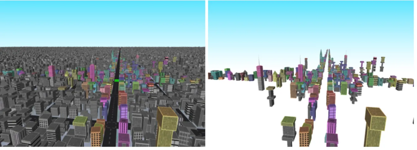
Occlusion culling is a fundamental problem in computer graphics. It removes objects that are occluded from the viewer in advance so that the graphics hardware does not need to render these invisible objects. Occlusion culling is very important when the graphics hardware ren-ders large and complex scenes with millions of polygons (Figure 1.1). While culling occluded objects from a single viewpoint is quite simple, many performance-critical applications require the potentially visible set (PVS) for a region in space to be computed, which is much more complicated. Among many excellent from-region visibility algorithms, visibility sampling has been shown a robust solution to PVS computation[BMW+09].

The basic idea of visibility sampling is to compute the visibility of a scene by sampling visibility interactions at discrete positions in the scene. It is critical to distribute samples in-telligently since the efficiency and accuracy of visibility computation are mainly determined by the position of samples. Recently, adaptive sampling techniques have become popular due to their efficiency on distributing samples. For example, object-space algorithms[WWZ+_06,

BMW+09] use ray casting to gather visible sets and iteratively find other visible objects by sampling their neighbors. Nirenstein et al.[NB04] proposed an image-space approach in which

Figure 1.1: A complex urban scene. Left: Only a small part of the scene (colored part) is visible if the viewer is on the road (the green area). Right: The visible set of the scene. [LSCO03]

they adaptively sample visibility based on the image differences between two rendered images of the PVS and the original scene. While the image-space approach is computationally more efficient, it is less accurate as scene geometry information is not exploited to distribute samples. In this thesis, we proposed an image-space visibility sampling approach that utilizes depth and color information to improve the efficiency and accuracy of PVS computation and make the visual errors unnoticeable. Unlike the image-space sampling approach[NB04] that places sam-ples only based on the visual error of existing samsam-ples, we further utilize the depth information to predict the visibility at positions that have not been sampled and distribute samples at regions where more samples are needed. Our motivation is that in a scene with complex occlusions, it is difficult to predict visibility at unsampled regions using the visibility at sampled regions as the visibility varies dramatically at different locations. To resolve this difficulty, we use the depth information to predict the visibility at unsampled regions. In particular, large depth change mostly means there is a gap in the scene, e.g., narrow lanes in urban scenes or hallways in indoor scenes. In the image-space sampling approach, these gaps are often undersampled and thus causing visual errors. On the contrary, our approach utilizes the depth information to guide samples to an appropriate position to include more visible objects. In the other hand, sometimes the visual errors are difficult to be noticed, such as forests with trees and plenty of

1.1 Contribution 3

small leaves, or a crowd of people in diverse dressing. The complex appearances of objects let these errors hard to be found. It’s not necessary to put many samples on such places with unnoticeable errors. Surprisingly, few methods have considered the object appearances, such as colors and textures, into their sampling mechanisms. To achieve this, we also utilize the image errors caused by the object appearance to judge the contribution of samples to prevent the over-smapling. It is noteworthy that although we compute visibility in the image space, our approach utilizes the depth information, which makes our algorithm somewhat similar to the object space approaches[WWZ+06, BMW+09] and the accuracy of PVS computation is improved.

Our experiments demonstrate that our sampling algorithm can discover more visible objects in the depth gaps and thus increase the PVS accuracy. Besides, image error of occlusion culling is controllable and the fast computational speed of the proposed algorithm makes it suitable for real-time applications such as games, visualizations, line-of-sight analysis and virtual reality.

1.1

Contribution

Our main contributions is:

• Proposing to combine the strengths of image-space and object-space visibility sampling algorithm by assisting image-space sampling with scene depth.

• Introducing the concept of actively predicting the visibility at unsampled region besides passively adding samples based on the PVS at sampled region.

• Proposing an importance sampling approach that effectively improves the efficiency and accuracy of visibility sampling for the aggressive occlusion culling problem.

1.2

Organization of the thesis

The following chapters are organized as follows. Chapter 2 gives the literature review and the background knowledge. Chapter 3 introduces the definition of the visibility importance

func-tion and how to evaluate it. Chapter 4 describes our aggressive visibility sampling algorithm, including the overview, hierarchical space partition, and the visibility computation framework. Chapter 5 shows the experimental results of our visibility sampling algorithm and comparison to several algorithms. Finally, we summarize our visibility sampling algorithm and discuss the future works in Chapter 6.

C H A P T E R

2

Related Work

Occlusion culling has been widely studied in computer graphics for many years. Existing oc-clusion culling approaches can be classified by whether the visibility is computed from a point or a region. Since our algorithm is a from-region approach, we only review few remarkable point-based methods in this section. Our review will focus on the region-based methods. For a comprehensive survey on occlusion culling approaches, we refer the interested readers to [COCSD03].

2.1

Point-based Visibility

Point-based methods try to find the visible set from a point, i.e. from the camera position. Since the camera position is unknown in advance, the visibility can only be computed on-the-fly during the real time walk-through. However, using the traditional Z-buffer for occlusion test in a large scene is inefficient. Greene et al. [GKM93] proposed a Hierarchical Z-Buffer (HZB) method to reuse the Z-buffer data and perform the occlusion test hierarchically. The scene is partitioned into an oct-tree, and a Z-pyramid is also built. In the Z-pyramid, each pixel in the

upper level contains the maximum depth of the 4 pixels in the lower level. The oct-tree nodes are tested hierarchically with the Z-pyramid during the occlusion test, and thus it can remove the ccludee quickly. Later Zhang et al. [ZMHH97] proposed the Hierarchical Occlusion Maps (HOM) which was extended from HZB. The main difference is that HOM simply fills a white pixel into an occlusion map when Z-buffer is updated (Figure 2.1). Also the occlusion pyramid is built but HOM uses the average operation during down sampling, and thus this can be done with hardware mip-map. During the occlusion test, the bounding boxes are projected into the occlusion map and the overlapping pixels are scanned recursively. If any one of the overlapping pixels is not completely opaque in the lowest HOM level, the box is rendered. Although it has to select a set of occluders to built the HOM, this method can provide aggressive visibility by simply changing the opaque threshold.

2.2 Region-based Visibility 7

2.2

Region-based Visibility

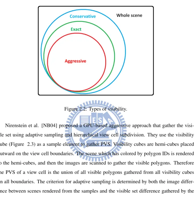
According to the correctness of the visibility, from-region visibility approaches can be fur-ther categorized into three types: exact, conservative, and aggressive (Figure 2.2). Exact solutions[NBG02] try to find the exact visible set of a region; however, their computational cost is high and robustness is not proven for large complex scenes. Although some acceleration techniques for exact approaches have been proposed[LSCO03, BWW05], the assumption on the scene geometry restricts the application of these techniques. Conservative solutions[WWS00, DDTP00] ensure the correctness of the potentially visible set(PVS). That is, no visible objects will be lost in PVSs generated by a conservative approach, but some objects that are occluded may be erroneously included in the PVSs as well. As the large overestimation of the PVS could cause low culling efficiency, conservative solutions are not appropriate for speed-critical applications such as games and virtual reality. In contrast to conservative approaches, PVSs produced by aggressive approaches are never overestimated. Thus, no occluded objects would be included in the PVSs. Although aggressive approaches may cause some visual errors such as missing objects due to underestimated PVSs, they are more efficient computationally and thus more suitable for interactive or realtime applications. For this reason, recent research on aggressive visibility approaches has focused on minimizing the visual errors of PVSs.

Figure 2.2: Types of visibility.

Nirenstein et al. [NB04] proposed a GPU-based aggressive approach that gather the visi-ble set using adaptive sampling and hierarchical view cell subdivision. They use the visibility cube (Figure 2.3) as a sample element to gather PVS. Visibility cubes are hemi-cubes placed outward on the view cell boundaries. The scene which has colored by polygon IDs is rendered to the hemi-cubes, and then the images are scanned to gather the visible polygons. Therefore the PVS of a view cell is the union of all visible polygons gathered from all visibility cubes on all boundaries. The criterion for adaptive sampling is determined by both the image differ-ence between scenes rendered from the samples and the visible set differdiffer-ence gathered by the samples, respectively. When the image difference is large, more samples are added recursively until the predefine threshold is met (Figure 2.4). View cells are recursively subdivided during the sampling until the PVS size is smaller than a threshold, and samples are also added to the subdivision plane in order to have the visible set more precise (Figure 2.5). However, as Niren-stein et al. do not take the scene geometry information into account in their adaptive sampling process, the number of samples increases drastically because of their sampling mechanism.

2.2 Region-based Visibility 9

Figure 2.3: Left: Visibility cubes. Right: Visibility cubes on the view cell boundaries. [NB04]

Figure 2.4: Left: Uniform sampling. Right: Adaptive sampling. [NB04]

Figure 2.5: Left: The subdivision plane (green). Right: New samples added on the subdivision plane. [NB04]

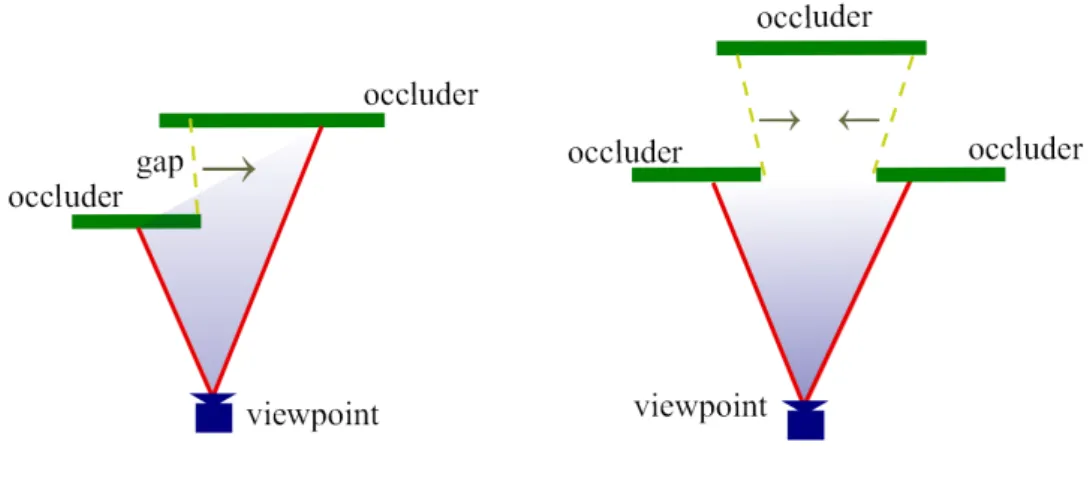
Wonka et al.[WWZ+06] proposed Guided Visibility Sampling (GVS) using ray-casting to generate polygon-based aggressive PVSs. Their sampling scheme exploits the property of ge-ometry adjacency. They use adaptive border sampling and reverse sampling to deal with the

scenes with complex occlusions. When a ray hit a new visible polygon, a border polygon with 9 edges is created by extending the new visible polygon(Figure 2.6 middle top). Then more rays are cast toward all vertices of the border polygon . If two rays cast to the ends of an edge hit different polygons, a new ray is cast to the center of the edge(Figure 2.6 left bottom). Samples are added recursively until the two neighbor rays hit the same polygon. Although the adaptive border sampling can find the neighbor polygons, some gaps can’t be penetrate. In Figure 2.7, predicted(x) is a point that should be pass thought by a new ray calculated by the adaptive border sampling, and hit(x) is the point actually hit by the ray. If hit(x) is too far from predicted(x), the reverse sampling is performed. A new point pnew (the yellow

point in Figure 2.7) is selected and a new ray sample is cast starting from the intersection of line(pnew, predicted(x)) and the view cell boundary, and toward pnew. If the starting point is

not on the view cell boundary, the sample is invalid.

2.2 Region-based Visibility 11

Figure 2.7: Reverse sampling. [WWZ+_06]

Bittner et al.[BMW+_{09] proposed another ray-casting aggressive algorithm, Adaptive Global}

Visibility Sampling (AGVS), to compute object-based visibility. They introduced a new con-cept of the global visibility in which the sampling mechanism can gather visible objects to multiple view cells simultaneously, and progressively updates the PVSs of all view cells in the scene. The PVS accuracy is not only considered each cell locally, but also all cells in the scene globally. Similar to GVS, the strategy to allocate rays also exploits the property of geometry adjacency, trying to find more visible objects near the current visible objects. In order to reduce visual errors, they use visibility filtering to include objects near the visible objects whether they can be seen or not. However, this could make the final PVS more conservative.

Figure 2.8: Adaptive global visibility sampling (AGVS). The contribution of a ray can affect multiple view cells. [BMW+_09]

Although both [WWZ+_{06] and [BMW}+_{09] are aggressive solutions, the differences}

be-tween ray-casting and image-based methods result in different characteristics of visibility. As mentioned in [WWZ+06], ray-casting methods try to find visible objects as precisely as possi-ble, but image-based methods aim to increase the rendering speed by removing occluded and even visually insignificant objects.

C H A P T E R

3

Visibility Importance

Sampling

In this section we introduce our visibility sampling algorithm by firstly giving an overview and then describing each step of our sampling algorithm. Our sampling approach is a from-region aggressive occlusion culling approach for a general 3D scene with predefined view cells. It out-puts a polygon PVS for each view cell. Although there is no restriction about the shape of view cells, we use box shaped cells with rectangular boundaries in our implementation. We define an importance function to guide sampling positions. For each boundary face of a view cell, an im-portance function is built according to the depth and color information of samples distributed on the boundary face. Since visibility discontinuities often occur at locations with large depth vari-ations, e.g., streets between buildings or a hallway between walls, depth gradients is computed to discover potential locations that have more visible polygons. Hence, more samples should be distributed at regions with large depth gradient to acquire more accurate PVS. However, some visual errors are not noticeable when they lie to the places with complex color variations, and it’s unnecessary to place too many samples there. Therefore we consider whether these errors

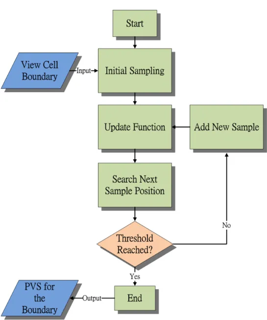
are noticeable or not by calculating the color differences between the visible objects and PVS in a textured scene. This color difference can determine how significant are the visual errors at the sample. If the color difference is large, more samples should be placed nearly. We combine both depth and color information to build the importance function to guide sampling positions. Our sampling algorithm operates as follows. At the beginning, we initialize the importance function by uniformly placing samples (3x3 to 5x5 grid) on each boundary face of a view cell. Then we iteratively search for the optimal location to place the next sample based on the sample importance function, compute the sample information, and update the importance function until a predefined error threshold is reached or the number of samples exceed a predefined limit. After sampling all boundary faces of a view cell, the union of visible polygons of all samples on all boundary faces is the PVS of the view cell.

The following is the procedure for sampling a view cell boundary (Figure 3.1): 1. Initially sample the boundary and update the importance function.

2. Search for the optimal position based on the importance function.

3. Add a new sample on the optimal position and compute visible polygons and the depth information.

4. Update the importance function with the new sample. 5. Repeat steps 2 to 4 until the threshold is reached.

3.1

Visibility Cube

We adopt the visibility cube[NB04] as the basic sampling element in our sampling algorithm. The visibility cube is a hemi-cube placed on an outside face of a cell. For each of the five faces of a hemi-cube (front, up, down, left, and right), a camera is placed and view outward (toward the scene). The images rendered from these cameras with depth test enabled are the visible set

3.1 Visibility Cube 15

from the sampled position. Each polygon in the scene is shaded with a unique color to denote the index of the polygon. After images viewed from all five cameras on a hemi-cube are ren-dered, pixel colors on these images are traced in order to find the visible polygons. In additional to polygon indices, we also use the visibility cube to render other information including depth and textured appearance for the importance computation later. Theoretically, the image is the exact visible set of the sample, but practically, there may exist sampling error since thin or small polygons may be lost after rasterization due to problems such as resolution, field of view dif-ferences, or frustum setting. To reduce these sampling errors, higher resolution of hemi-cube images can be used by sacrificing some computational speed; nevertheless, as most of those tiny polygons are not perceptually visible, the decision usually favors computational performance instead of accuracy. This is especially true for real-time applications because it is computation-ally expensive to render the conservative or exact PVS of a complex scene. Therefore, these visually unimportant polygons can be ignored to improve computational performance.

3.2

Sample Importance Function

As visibility changes drastically at the place where the depth from a sampled camera position varies greatly or is discontinuous, we define the importance of a sample by measuring the depth variations on all five faces of the sample’s hemi-cube. More specifically, the importance of a sample s is the sum of the importance of all pixels of the five hemi-cube images:

Is(s) = C N

X

i=1

Ip(xi), (3.1)

where C is a scalar factor that decided by the averaged pixel color difference between the image rendered with current view cell PVS and the exact visible set image (rendered with the whole scene). Each image is rendered with textured scene. The color differences are calculated in R, G, B separately and averaged together into a scalar value. By control the value of C, we can enlarge and reduce the importance according to the color differences. Ip(xi) is the importance of

3.2 Sample Importance Function 17

Figure 3.2: Left: Visibility cube samples on boundary faces of a view cell. There are 4 visibility samples on each boundary face in this case. Right: Each sample has a hemi-cube consisted of 5 images. Every polygon has an unique color in order to be recognized when gathering visible set.

is normalized to [0, 1]. The importance of a pixel is a 4D vector containing depth differences between x and its four immediate neighbors: xr, xu, xl, and xd corresponding to the right, up,

left, and down direction, respectively. That is, the importance of a pixel is defined as a weighted depth gradient at x in four directions:

Ip(x) = 1 d(x)         wr(d(xr) − d(x)) wu(d(xu) − d(x)) wl(d(xl) − d(x)) wd(d(xd) − d(x))         , (3.2)

where d(x) is the depth value at pixel x normalized by the far plane distance. wr, wu, wl, and wd

are the 2D distance from x to the left, bottom, right and top border of the image, respectively. wr, wu, wl, and wd are used to enhance the influence of pixels that are close to the boundary

far-Figure 3.3: Left: A depth gap in the view volume. The right occluder is farther causing the gap facing the lower-right direction, so the viewpoint should move toward the right direction in order to see larger area in the gap. Right: The direction of the two gaps are opposite. After combining the contribution of two gaps, the viewpoint will not move as the facing direction of two gaps are opposite.

ther from the position of the current sample. Once the sample importance function is defined, the visibility importance function can be constructed using the importance of samples on the boundary of a view cell.

3.3

Visibility Importance Function

Theoretically, to obtain the exact visibility set viewing from a boundary face of a cell, the boundary face has to be filled with an infinite number of samples; however, it is neither feasible nor efficient to distribute infinite samples in practice. We can only have finite discrete samples to obtain an aggressive PVS of a view cell. If we place a camera at a position that has not been sampled, the visible set may be neither 100% exact nor reliable enough for occlusion culling. The reliability of an aggressive PVS may be even lower in a scene that has complex occlusion and depth variation. In order to increase the reliability, samples should be put at those locations with lowest reliability.

3.3 Visibility Importance Function 19

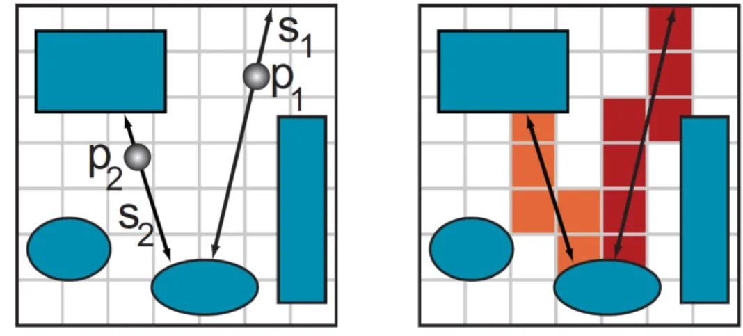
The visibility importance function is a 2D function defined on the boundary faces of a view cell. The function returns a scalar value ranging from 0 to 1 to represent the reliability of the current PVS at some locations of boundary faces. The reliability is 1.0 at a position that has been sampled, and decreases as the sample importance of sample decreases or the distance to existing samples increases. Every time when a new sample is added, the visibility importance function is updated as follows:

R(p) = (1 − α)e− kp−sk2 σ2 H(p,s) + αe −kp−sk2 σ2 V(p,s), (3.3)

where p is a 2D position on a boundary face at which the visibility importance function would be updated and kp − sk is the Euclidean distance between p and a sampled 2D position s. α is the horizontal component of the vector p − s. Moreover, σH(p, s) and σV(p, s) are defined by

σ_H2(p, s) =    1 − Is,l(s), if p is at left side of s 1 − Is,r(s), if p is at right side of s (3.4) σ2_V(p, s) =   

1 − Is,u(s), if p is at upper side of s

1 − Is,d(s), if p is at lower side of s,

(3.5)

where Is,r(s), Is,u(s), Is,l(s) and Is,d(s) are the 1st, 2nd, 3rd, and 4th component of Is(s),

respectively. σH(p, s) and σV(p, s) are determined by the relative position of p and s. For

example, if p is on the upper-left side of s, then σH(p, s) = 1−Is,l(s) and σV(p, s) = 1−Is,u(s).

The reliability R(p) decreases exponentially as the importance of the sample s increases or the distance to the sample s increases. This is because that larger sample importance means there is a larger depth discontinuity and image difference, and the reliability should decrease accordingly. Therefore, more samples should be placed nearby. During the updating process, we update the visibility importance function only when a new sample at p increases the reliabil-ity; otherwise, the importance function will not be updated because other pre-existing samples provide higher reliability for the current PVS. In Figure 3.4, the red sample has higher impor-tance value than the blue one, so the PVS reliability of the red sample decreases faster than the blue one. That is, there are more samples needed near the red sample.

After the visibility importance function is updated, we need to choose a new sampling po-sition. To raise the PVS reliability, samples should be located at positions with low reliability. Hence, we search for the global minimum of the visibility importance function and use it as the next sampling position. We iteratively compute the new sample, update the visibility impor-tance function, and search for the optimal sampling position until the visibility imporimpor-tance of the whole scene is higher than a predefined reliability threshold, or the total number of samples exceeds a preset number. After all boundaries of the view cell are completely sampled, the union of all visible set of all samples is the PVS of the view cell.

3.3 Visibility Importance Function 21

Figure 3.5: Left: The samples (purple dots) on the view cell boundary (blue rectangle). Right: The PVS reliability distribution of the boundary.

4

Visibility Computation

Framework

To validate the efficiency and accuracy of our visibility sampling algorithm, we develop an aggressive region-based occlusion approach based on it. This occlusion culling approach takes a general 3D polygon scene and view cells as inputs and produces a PVS for each view cell. We describe the implementation details of our occlusion culling approach in this section. The major steps of our occlusion culling approach are as follows (Figure 4.1):

1. Construct a hierarchical space partition for the input scene.

2. For each view cell, perform visibility importance sampling on all boundary faces. 3. Merge the contributions of all samples of a cell.

4. Repeat step 2 and 3 until the PVSs of all cells are computed.

23

4.1

Hierarchical Space Partition and View Cells

In order to improve the computational performance of sampling, we build a hierarchical space partition tree for the scene according to the number of polygons in each partition. For general urban scenes, the horizontal space is much larger than the vertical space, so we use a quad-tree hierarchy to partition the 2D horizontal space in our implementation. We typically set 10,000-50,000 polygons as the number of polygons for each partition. We also utilize this hierarchy to quickly get rid of invisible polygons for each sample using view frustum culling. This accelerate the scene rendering during the sampling process.

The view cells in our sampling algorithm can be any shape as long as their boundary faces have a finite area. Shapes that have no boundary such as spheres cannot be used in our sampling algorithm. For simplicity of implementation, we use axis-align boxes as view cells. Although there is no restriction on where to place view cells, we only put view cells on regions where the user can navigate. For urban scenes, outdoor roads are ideal view cell locations. It is not necessary to put cells inside the buildings, above the sky, or underground. The size of view cells can vary according to the scene and application. In our experiments, we typically set the size of view cells about 10-20 meters wide and 5-10 meters long.

4.2

Visibility Sampling

When the visibility cube is used to compute the sample contribution, image resolution is a crucial parameter for controlling the quality and computational time. In our experiments, we set the image resolution at 1024 × 1024 as this setting balances visual quality and computational speed. We can choose 512 × 512 for faster computational performance or 2048 × 2048 to reduce image error. As the 5 images should be combined into a hemi-cube, the field-of-view angles of all images are 90 degrees. Moreover, to save the memory storage of 5 hemi-cube images, only the front camera of the hemi-cube renders a full image, while the other 4 cameras render 4 half images. Thus all five cameras only occupy 3 full images. The index for identify polygons is

4.3 Computing Importance Function 25

a 24-bit integer representing a RGB color, so the index number can be up to 16 millions. The index is used as the polygon color when the GPU rendering polygons. We also compute the depth gradient using the GPU shader programs when rending the images and store the scene images together with the depth gradients in a multiple render target (MRT). After complete rendering, the results are sent back to the CPU and all pixels are checked to compute visible polygons and importance values of samples.

4.3

Computing Importance Function

The importance function is stored in a 2D floating-point array. Each element represents a pos-sible sample position on a boundary face. The size of array affects how densely a boundary can be sampled. In our experiments, we found that a 2562 _{array generally provides enough}

spatial resolution for sampling. The importance function should be updated using equation 3.3 every time a camera sample is computed. In practice, we only update function values near the updated sample since the exponential function in equation 3.3 decreases rapidly. When the boundary face is not a square, the updating value and range should be modified according to the aspect ratio of the boundary face and the array of importance function. The updating process of importance function is also done by the GPU shader program. The visibility importance function represents the reliability of current PVS, so the position with lowest function value is the next optimal sample position. We search for the minimum of the function efficiently using the min-max mipmap on the GPU.

5

Results

We evaluated our visibility sampling algorithm by testing it on two versions of Vienna City model1_{: one with 800 thousand and the other with 8 million polygons (Figure 5.1 and Figure}

5.2), and the Hong Kong City2 _{model with 2 million polygons (Figure 5.3). We also compare}

the computational performance, PVS accuracy, and image error of our algorithm with those of the adaptive sampling method proposed by Nirenstein and Blake[NB04] (NIR04) and the Guided Visibility Sampling (GVS) proposed by Wonka et al. [WWZ+06] which is an object-based method. All timings are measured on a PC platform with an Intel Core 2 Duo 2.66GHz CPU, 3GB RAM, and an NVIDIA GTX260 graphics card. We implement our programs with OpenGL and GLSL. The image resolution of visibility cubes are 1024 × 1024, and the impor-tance function uses 256 × 256 arrays, and the image resolution is 1024 × 1024 for image error tests in all experiments.

1_{http://www.cg.tuwien.ac.at/research/vr/urbanmodels/index.html} 2 _{International Games System CO., LTD.c}

5.1 Performance Comparison 27

Figure 5.1: The Vienna City model we tested. The polygon count of Vienna800K and Vi-enna8M are 865,979. The positions we choose as view cells include open squares, narrow lanes, and crossroads.

5.1

Performance Comparison

Table 5.1, 5.2, and 5.3 show the performance comparison of our algorithm with NIR04 and GVS. We choose 20 typical view cells at certain places such as crossroads, narrow lanes, and open squares for testing and compute the average of the data measured at these view cells. The Vienna800K model has textures so we test it with both depth guided and depth+color guided. The Vienna8M and Hong Kong model don’t have textures so we only test them with depth information (set C = 1 in Equation 3.1). Although the threshold of our method which means the PVS reliability can be specified by the user, for comparison with NIR04, we directly control

Figure 5.2: Another version of Vienna City model (Vienna8M) which has 7,928,519 polygons.

the number of samples to match the number of samples that NIR04 used. Each scene we set 2 different thresholds to generate different results with high and low sample counts by NIR04. GVS uses ray casting to gather visible sets so the numbers of samples are greatly different from those of image-based approaches. Typically millions of rays are needed for a PVS for a view cell with an acceptable error rate. Since we just realize a basic ray caster with a hierarchical space partition and it is not optimized in detail, we mainly compare the PVS accuracy and image error with GVS. The visible set percentage at each tables is defined as the number of polygons in the PVS divided by the total number of polygons in the scene. As no false visible

5.1 Performance Comparison 29

Figure 5.3: The Hong Kong City model which has 2,164,567 polygons.

polygons would be included in the PVS of aggressive visibility, higher visible set means higher accuracy. In each test, we measure the averaged pixel error rate to show the accuracy practically. Since Vienna800K has textures, we further measure the averaged color error of false pixels by calculating R, G, B differences respectively. The color error rates can show how visually significant the error pixels are.

One can observe that our algorithm can gather more visible objects under similar number of samples in Vienna800K (see Exp 3 vs. Exp 5 and Exp 4 vs. Exp 4 in Table 5.1). Also, our method requires fewer samples and shorter computational time while achieving similar PVS

accuracy as NIR04 (see Exp 2 vs. Exp 7 in Table 5.1). When considering the effect of color differences in a textured scene (Exp 5 and Exp 6 in Table 5.1), our method can further find more visible objects under the same number of samples despite the increasing of the computation time.

Although the Vienna8M model has more complex occlusions that cause lower visible set percentages, our algorithm still outperforms NIR04 (Table 5.2). For scenes that actually used in video games like the Hong Kong model (Table 5.3), our method also outperforms NIR04 under the similar number of samples. Figure 5.4 shows the PVS distribution produced by our method compared with NIR04. Generally our method can find more visible polygons under similar number of samples

Due to the aggressive property, there is no false visible objects in a PVS. Higher visible set percentage also potentially means lower visual error when rendering with the PVS. The pixel error rates shown in each tables show that our method provides lower pixel error rates compared with NIR04 under similar samples. Compared with GVS under the similar visible set percentage (Exp. 1 vs. Exp. 9 in Table 5.1), our method also provides a better visual accuracy. Since we consider the texture information, the color error rates are lower than methods that don’t consider textures.

In Vienna800K and Hong Kong the image-based methods gather larger visible sets than GVS, but GVS finds more visible objects in Vienna8M model. The reason is the wide range of Vienna8M. Ray casting can find any polygons that can be seen theoretically from the view cells no matter how far they are. However, in practice these polygons may be smaller than a pixel on the screen so they are almost invisible. The pixel error test results in Table 5.2 show that the image-based method like our method and NIR04 incur fewer visual errors compared with the object-based method GVS even if GVS gather much more visible object. The reason is the wide range of Vienna8M and many polygon found by GVS are too far and tiny to be noticed from the view cells. The different characteristics of image-based and object-based methods cause different visual accuracies.

5.2 Image Error and PVS Accuracy 31

Table 5.1: Comparison of performance, PVS accuracy, and visual error of our method and Nirenstein and Blake’s method [NB04] and Wonka et al.’s method [WWZ+06] in the Vi-enna800K model.

Exp. Method Samples/Cell Time/Cell Visible Set Pixel Error Color Error 1 Depth 80 6.22s 2.80% 5.5 × 10−5 1.5 × 10−5 2 Depth 180 15.47s 3.05% 4.0 × 10−6 1.2 × 10−6 3 Depth 264 22.96s 3.13% 2.0 × 10−6 5.6 × 10−7 4 Depth 320 35.35s 3.17% 2.0 × 10−6 5.5 × 10−7 5 Depth + Color 264 115.33s 3.15% 2.0 × 10−6 5.7 × 10−7 6 Depth + Color 320 142.48s 3.18% 1.0 × 10−6 5.4 × 10−7 7 NIR04 266 18.88s 3.04% 2.2 × 10−5 6.0 × 10−6 8 NIR04 324.6 23.66s 3.08% 1.6 × 10−5 4.7 × 10−6 9 GVS 7.25M 175.61s 2.70% 3.1 × 10−4 9.9 × 10−5

GVS. The reason is that polygons in Hong Kong are relative discrete than others, and there are many overlapping polygons causing severe z-fighting phenomenon. These are unfavorable for ray casting approaches like GVS. However, image-based methods can sustain discrete or overlapping polygons without introducing too much error since every sample is a larger scale of view rather than a smaller scale ray so it can gather a bulk of visible objects once.

5.2

Image Error and PVS Accuracy

We give some real examples of pixel error of our method compared with NIR04 and GVS. In each pixel error images rendered with PVS produced by each methods, blue pixels are correct while red pixels are false pixels (false invisible). Figure 5.5 shows some examples of error pixels of our methods. Most of these errors result from projection, resolution, and field of view settings. As these error pixels are tiny and located in far distances, so they are hardly noticeable if their pixel color was not highlighted. Figure 5.6, 5.7, and 5.8 are 3 different views

Table 5.2: Comparison of our method with NIR04 and GVS in the Vienna8M model. Exp. Method Samples/Cell Time/Cell Visible Set Pixel Error

1 Depth 176 66.22s 0.413% 1.1 × 10−5 2 Depth 296 111.70s 0.433% 6.0 × 10−6 3 NIR04 176.3 48.67s 0.407% 6.3 × 10−5 4 NIR04 301 86.31s 0.431% 4.9 × 10−5 5 GVS 5.4M 369.91s 1.27% 1.4 × 10−4

Table 5.3: Comparison of our method with NIR04 and GVS in the Hong Kong model. Exp. Method Samples/Cell Time/Cell Visible Set Pixel Error

1 Depth 284 51.97s 1.77% 8.8 × 10−5 2 Depth 424 79.39s 1.86% 4.9 × 10−5 3 NIR04 288 36.22s 1.68% 4.4 × 10−4 4 NIR04 427 54.19s 1.80% 2.4 × 10−4 5 GVS 14.3M 777.31s 1.80% 3.4 × 10−3

rendered by PVS produced by our method and NIR04. NIR04 is also an image-based approach, the errors incurred by projection and resolution are exist, too. However, since we considered the geometry and texture information, the errors incurred by our method are fewer at the far distance compared with NIR04.

Although the PVS produced by GVS has higher visible set percentage in Vienna8M (Exp.5 in Table 5.2), it doesn’t outperform ours and NIR04 in aspect of image error. Figure 5.9, 5.10, and 5.11 are examples of pixel error incurred by our method and GVS. In our experiments, GVS tends to lose some visually important polygons but gather far and tiny polygons. This is caused by the characteristic of object-based ray casting method we mentioned before. In Figure 5.12 we place the camera out of the view cell (the green wired box). The PVS produced by GVS has a lot of tiny polygons far from the view cell, while our method mostly find polygons near the view cell. Although these far polygons are visible theoretically, these unnoticeable polygons

5.2 Image Error and PVS Accuracy 33

may cause rendering overhead and hit performance during real-time applications.

In order to test the accuracy of the sampling mechanism, we continuously add samples on a boundary face of a view cell. The relationship between the growing number of samples and the PVS size of the sampling results on 5 different boundary faces is shown in Figure 5.13. One can observe that the PVS size grows rapidly when the number of samples is less than 100 and almost capture all visible objects afterward. This shows that our sampling algorithm is very efficient to distribute samples.

(a) Vienna800K

(b) Vienna8M

(c) Hong Kong

Figure 5.4: The PVS distribution produced by different methods in different view cells of dif-ference scenes.

5.2 Image Error and PVS Accuracy 35

(a)

(b)

Figure 5.5: (a) A view at a crossroad (b) The same scene rendered using the PVS generated by our algorithm, where blue pixels are true visible objects and red pixels show image errors (false invisible objects).

Figure 5.6: Top: a view in Vienna800K. Bottom left: Pixel errors of PVS of our methods. Bottom right: Pixel errors of PVS of NIR04.

5.2 Image Error and PVS Accuracy 37

Figure 5.7: Top: another view in Vienna800K. Bottom left: Pixel errors of PVS of our methods. Bottom right: Pixel errors of PVS of NIR04.

Figure 5.8: Top: a view in Vienna8M. Bottom left: Pixel errors of PVS of our methods. Bottom right: Pixel errors of PVS of NIR04.

5.2 Image Error and PVS Accuracy 39

Figure 5.9: Top: a view in Vienna800K. Bottom left: Pixel errors of PVS of our methods. Bottom right: Pixel errors of PVS of GVS. There are significant polygons missed.

Figure 5.10: Top: a view in Vienna8M. Bottom left: Pixel errors of PVS of our methods. Bottom right: Pixel errors of PVS of GVS. There are significant polygons missed.

5.2 Image Error and PVS Accuracy 41

Figure 5.11: Top: a view in Hong Kong. Bottom left: Pixel errors of PVS of our methods. Bottom right: Pixel errors of PVS of GVS. There are significant polygons missed.

Figure 5.12: Top: a top view in Vienna8M. The camera is placed out of the view cell (the green wired box). Bottom left: The polygons found by our method are near the view cell. Bottom right: GVS found many far and tiny polygons from the view cell.

5.2 Image Error and PVS Accuracy 43

Figure 5.13: This figure shows that our sampling algorithm is very efficient on placing samples. One can observe that the PVS size grows rapidly when the number of samples is less than 100 and the PVS almost captures all visible objects afterward.

6

Conclusions

In this chapter, we give a brief summary and conclusion about our visibility computation algo-rithms. We also several directions for future improvements.

6.1

Summary

We present an aggressive region-based visibility sampling algorithm for general 3D scenes. Rather than adding visibility samples only based on the visual error of the PVS of sampled regions, we actively estimate the reliability of the visibility at unsampled position and add samples at low reliability regions. Our algorithm utilizes the depth gradients to construct an importance function that represents the reliability of the potentially visible set (PVS) on a view cell’s boundary faces. The importance function guides visibility samples to depth discontinu-ities of the scene such that more visible objects can be sampled to reduce the visual error. Our experiments show that our sampling approach can effectively improve the PVS accuracy and computational speed compared to the image-based adaptive approach proposed in [NB04] and the object-based approach proposed in [WWZ+06].

6.2 Limitations and Future Work 45

6.2

Limitations and Future Work

Although the depth gradient is an important information to guide samples into better positions, the PVS and the visual errors are still crucial factors since they directly affect the accuracy of the visibility. However, unlike the depth information, the PVS doesn’t have a direction to provide a hint about sample positions. To utilize the information of the PVS in the precomputing phase more effectively is a critical issue to improve the accuracy. In the other hand, currently we only consider the visual errors in a simple way, to calculate the average difference. Further analyzing the visual information, such as the saliency of the image, better image error metrics, or introduce more methods about perception, vision, and image processing, may help the efficiency of each sample.

Since we have defined a function in a 2D space on the cell boundaries to guide samples, it’s simple figure out that to extend this function into a 3D space containing the whole scene. This could be benefic since the contributions of all samples can affect each other and potentially a better sample distribution could be found globally. Also a better view cells distribution could be created simultaneously during the sampling process. However, this is difficult in several aspects. First the representation of the function has to be modified since the wide range of the whole scene. Therefore the method to compute the sample contributions and update have to be changed respectively. Then how to divide the function into view cells and distribute the PVS is another tough question. It’s hard to solve the problems above, but this idea is innovative.

Last but not the least, since the rapid growing of the computation power of graphics hard-ware, maximizing the utilization of graphics hardware is always a crucial task. Although the graphics hardware helps us greatly compute the PVS by rendering, many other tasks in our al-gorithm still rely on CPU. Hence to further boost the computation speed, several optimizations of algorithm and implementation have to be done to reach a higher parallel degree. After all, increasing the efficiency of sampling and boosting the computation are basic ways to obtain an accurate PVS.

[BMW+09] Jiri Bittner, Oliver Mattausch, Peter Wonka, Vlastimil Havran, and Michael Wim-mer. Adaptive global visibility sampling. ACM Transactions on Graphics, 28(3):1–10, 2009.

[BWW05] Jiˇr´ı Bittner, Peter Wonka, and Michael Wimmer. Fast exact from-region visibil-ity in urban scenes. In Rendering Techniques 2005 (Proceedings Eurographics Symposium on Rendering), pages 223–230, 2005.

[COCSD03] Daniel Cohen-Or, Yiorgos L. Chrysanthou, Claudio T. Silva, and Fredo Durand. A survey of visibility for walkthrough applications. IEEE Transactions on Visu-alization and Computer Graphics, 9:412–431, 2003.

[DDTP00] Fr´edo Durand, George Drettakis, Jo¨elle Thollot, and Claude Puech. Conservative visibility preprocessing using extended projections. In SIGGRAPH 2000, pages 239–248, 2000.

[GKM93] Ned Greene, Michael Kass, and Gavin Miller. Hierarchical z-buffer visibility. In SIGGRAPH ’93: Proceedings of the 20th annual conference on Computer graph-ics and interactive techniques, pages 231–238, New York, NY, USA, 1993. ACM. [LSCO03] Tommer Leyvand, Olga Sorkine, and Daniel Cohen-Or. Ray space factorization

for from-region visibility. ACM Trans. Graph., 22(3):595–604, 2003.

Bibliography 47

[NB04] S. Nirenstein and E. Blake. Hardware accelerated visibility preprocessing using adaptive sampling. In Renderinig Techniques 2004, pages 207–216, 2004. [NBG02] S. Nirenstein, E. Blake, and J. Gain. Exact from-region visibility culling. In

EGRW ’02: Proceedings of the 13th Eurographics workshop on Rendering, pages 191–202, 2002.

[WWS00] Peter Wonka, Michael Wimmer, and Dieter Schmalstieg. Visibility preprocess-ing with occluder fusion for urban walkthroughs. In Renderpreprocess-ing Techniques 2000 (Proceedings Eurographics Workshop on Rendering), pages 71–82, 2000.

[WWZ+06] Peter Wonka, Michael Wimmer, Kaichi Zhou, Stefan Maierhofer, Gerd Hesina, and Alexander Reshetov. Guided visibility sampling. ACM Transactions on Graphics, 25(3):494–502, 2006.

[ZMHH97] Hansong Zhang, Dinesh Manocha, Thomas Hudson, and Kenneth Hoff. Visibility culling using hierarchical occlusion maps. Technical report, Chapel Hill, NC, USA, 1997.