繪圖處理器之材質貼圖下有效率之材質記憶體系統設計

國

立

交

通

大

學

資訊科學與工程研究所

碩

士

論

文

繪圖處理器之材質貼圖下有效率之材質記憶體系統

設計

The efficient texture memory system design for texture

mapping in GPU

研 究 生：張 辰 瑋

指導教授：鍾 崇 斌 博士

繪圖處理器之材質貼圖下有效率之材質記憶體系統

設計

The efficient texture memory system design for texture

mapping in GPU

研 究 生：張 辰 瑋 Student：

指導教授：鍾 崇 斌 博士 Advisor：Dr. Chung-Ping Chung

國 立 交 通 大 學

資 訊 科 學 與 工 程 研 究 所

碩 士 論 文

A Thesis

Submitted to Institute of Computer Science and Engineering

College of Computer Science

National Chiao Tung University

in Partial Fulfillment of the Requirements

for the Degree of

Master

In

Computer Science

July 2007

繪圖處理器之材質貼圖下有效率之材質記憶體系統

設計

摘 要

The efficient texture memory system design for texture

mapping in GPU

Student：Chen-Wei Chang Advisor：Dr, Chung-Ping Chung

Institute of Computer Science and Engineering National Chiao-Tung University

Abstract

Texture mapping is a common rendering technique in current Graphic Processing Unit architecture. In order to have better synthesized picture, many texture data will be referenced and accessed. We found that the technique may take significant part of total scene execution time on preliminary operations to access these referenced data. The operations could be coordinate generation, address translation and texels look up. And the time is increased as filtering algorithms are more complex.

In this thesis, we are going to improve this part of time (average texels access time of texture filtering) by proposing new texture placement under three possible and common texture cache supports. And the placement is target to achieve the goal by improving the texture cache hit rate, average cache access counts and address translation time.

As the result shows that the new placements could gain 2~9% upgrade in average texels access time of texture filtering under the three common texture cache support in current GPU architecture.

Contents

摘 要 ... I ABSTRACT... II CONTENTS...III LIST OF FIGURES ...V LIST OF TABLES... VII

CHAPTER 1 INTRODUCTION ... 1

-1.1MOTIVATIONS... -2

-1.2OBJECTIVES... -3

-1.3ORGANIZATION ABOUT THIS THESIS... -3

CHAPTER 2 BACKGROUND AND RELATED RESEARCH... 4

-2.1GPU RENDERING FLOW... -4

-2.2THE TEXTURE MAPPING TECHNIQUES... -5

2.2.1 The textures ... 6

2.2.2 Texture mapping process flow within Texture Unit... 6

2.2.2.1 Address translation ... 8 2.2.2.2 Texture filtering ... 9 -2.3RELATED RESEARCH... -13 2.3.1 Nonblock placement ... 13 2.3.2 4D placement... 14 2.3.3 6D placement... 16 CHAPTER 3 DESIGN... 18 -3.1DESIGN OVERVIEW... -18 -3.2TEXTURE PLACEMENT... -19 3.2.1 Recursive Z placement (RZ)... 19

3.2.2 Different placement policies... 21

3.2.2.1 Recursive Z with U (RZU) ... 21

3.2.2.2 Recursive Z with FlippedU (RZFU)... 22

3.2.2.3 Recursive Z with Snake (RZS) ... 23

3.2.3 Address translation idea of RZ ... 24

3.2.4 Address translation of other placements ... 29

3.2.5 Address translation logic implementation... 29

3.3.1 Baseline texture cache support ... 34

3.3.2 Texture cache support 1 ... 34

3.3.3 Texture cache support 2 ... 34

3.3.3.1 Possible design of texture cache support2 ... 35

3.3.3.1.1 Case identifier ... 35

3.3.3.1.2 Coordinate generator ... 38

3.3.3.1.3 Texels router ... 39

CHAPTER 4 EXPERIMENT AND RESULTS ... 43

-4.1 EXPERIMENT GOAL, ENVIRONMENT AND METHODOLOGY... -43

-4.2EXPERIMENT RESULTS... -44

4.2.1 Results of address translation time ... 45

4.2.2 Results under baseline texture cache ... 45

4.2.3 Results under texture cache support 1 ... 47

4.2.4 Results under texture cache support 2 ... 50

CHAPTER 5 CONCLUSION ... 52

-5.1CONCLUSION... -52

-5.2FUTURE WORK... -52

REFERENCE ... 53

APPENDIX ... 54

-A.1THE TIME DELAY OF MUX... -54

-List of Figures

FIGURE 2-1-1 RENDERING PIPELINE OF GPU... -4

-FIGURE 2-2-2-1 THE TEXTURE UNIT AND TEXTURE MAPPING PROCESSING FLOW... -7

-FIGURE 2-2-2-1-1 THE CONCEPT OF ADDRESS TRANSLATION. ... -8

-FIGURE 2-2-2-2-1 THE MIPMAPS AND DATA STRUCTURE OF A TEXEL... -10

-FIGURE 2-2-2-2-2 THE CONCEPT OF BILINEAR FILTERING... -11

-FIGURE 2-3-1-1NONBLOCK PLACEMENT AND ADDRESS TRANSLATION EQUATION... -13

-FIGURE 2-3-1-2 ACCESS CONDITION OF NONBLOCK PLACEMENTS... -14

-FIGURE 2-3-2-14D PLACEMENT AND ADDRESS TRANSLATION EQUATION... -14

-FIGURE 2-3-2-2 ACCESS CONDITION OF 4D PLACEMENT... -15

-FIGURE 2-3-3-1 THE RELATED WORK OF 6D PLACEMENT... -16

-FIGURE 3-2-1-1 RECURSIVE Z PLACEMENT... -19

-FIGURE 3-2-1-2 CROSS TILE CONDITION IN RZ AND 4D/6D... -20

-FIGURE 3-2-1-3 MULTIPLE CACHE LINES CONDITION IN RZ AND 4D/6D... -20

-FIGURE 3-2-2-1-1RECURSIVE Z WITH U PLACEMENT... -21

-FIGURE 3-2-2-2-1RECURSIVE Z WITH FLIPPED-U V1 ... -22

-FIGURE 3-2-2-2-2RECURSIVE Z WITH FLIPPED-U V2 ... -22

-FIGURE 3-2-2-3-1RECURSIVE Z WITH SNAKE PLACEMENT... -23

-FIGURE 3-2-2-1 DEFINITION OF TERMS... -24

-FIGURE 3-2-2-2 THE CASE I OF ADDRESS TRANSLATION... -24

-FIGURE 3-2-2-3 EXAMPLE OF ADDRESS TRANSLATION CASE I. ... -25

-FIGURE 3-2-2-4 THE CASE II OF ADDRESS TRANSLATION... -26

-FIGURE 3-2-2-5 EXAMPLE OF ADDRESS TRANSLATION CASE II ... -27

-FIGURE 3-2-2-6 THE CASE III OF ADDRESS TRANSLATION... -28

-FIGURE 3-2-2-7 EXAMPLE OF ADDRESS TRANSLATION CASE III... -28

-FIGURE 3-2-2-8 SUMMARY OF RZ ADDRESS TRANSLATION FUNCTION... -29

-FIGURE 3-2-5-1 CONCEPT OF ADDRESS TRANSLATION UNIT... -30

-FIGURE 3-2-5-2 GLOBAL VIEW OF ADDRESS TRANSLATION LOGIC... -31

-FIGURE 3-2-5-3 ONE CELL OF COMMON FIELD GENERATOR... -32

-FIGURE 3-2-5-4 COMMON FIELD GENERATOR WITH N CELLS... -32

-FIGURE 3-2-5-5 DIFFERENTIAL FIELD GENERATOR... -33

-FIGURE 3-3-3-1-1TEXTURE CACHE SUPPORT 2 ... -35

-FIGURE 3-3-3-1-1-1 MULTIPLE CACHE LINES CONDITIONS... -36

-FIGURE 3-3-3-1-1-2 OPERATION OF CASE IDENTIFIER... -36

-FIGURE 3-3-3-1-1-3 OVERVIEW OF CASE IDENTIFIER... -38

-FIGURE 3-3-3-1-2-1 OPERATION OF COORDINATE GENERATOR... -39

-FIGURE 3-3-3-1-3-2 OPERATION OF OFFSET GENERATOR... -41

-FIGURE 3-3-3-1-3-3BOOLEAN EQUATION OF OFFSET2... -41

-FIGURE 3-3-3-1-3-4BOOLEAN EQUATION OF ENABLE SIGNAL... -42

-FIGURE 4-2-1-1 ADDRESS TRANSLATION TIME OF DIFFERENT PLACEMENTS... -45

-FIGURE 4-2-2-1 MISS RATE IN BASELINE TEXTURE CACHE... -46

-FIGURE 4-2-2-2 CONFLICT MISS UNDER DIRECT MAPPING WITH 4D PLACEMENT... -47

-FIGURE 4-2-2-3 AVERAGE TEXELS ACCESS TIME OF BILINEAR FILTERING IN BASELINE TEXTURE CACHE SUPPORT-47 -FIGURE 4-2-3-1 AVERAGE CACHE ACCESS COUNTS IN TEXTURE CACHE SUPPORT 1... -48

-FIGURE 4-2-3-2 MISS RATE IN TEXTURE CACHE SUPPORT 1... -49

-FIGURE 4-2-3-3 AVERAGE TEXELS ACCESS TIME OF BILINEAR FILTERING IN TEXTURE CACHE SUPPORT 1 ... -49

-FIGURE 4-2-4-1 AVERAGE CACHE ACCESS COUNTS IN TEXTURE CACHE SUPPORT 2... -50

-FIGURE 4-2-4-2 MISS RATE UNDER TEXTURE CACHE SUPPORT 2 ... -51

-List of Tables

TABLE 2-2-2-2-1 SUMMARY OF TEXTURE FILTERING ALGORITHMS... -12

-TABLE 2-3-1 SUMMARY OF THREE PLACEMENT ALGORITHMS... -17

-TABLE 3-2-4-1SUMMARY OF LEAST SIGNIFICANT FOUR BITS OF ADDRESS AMONG PLACEMENTS... -29

Chapter 1 Introduction

In Three-Dimensional (3-D) computer graphics, texture mapping is a common and one of the successful techniques in high quality image synthesis. It is responsible for rendering the 3-D scene by adding detail, surface texture, pattern, surface normal or color to a 3-D object and become more and more complex due to the requirement of 3-D scene realism and special effect [1][2].

Basically, in order to have quality of synthesized image, more texels data will be referenced, and more computation will be invoked. We found that the complex texture mapping technique may take a significant part of scene total execution time on the preliminary operations. The operations are accessing the required referenced texels data in the texture memory system for texture filtering. They contain address calculations, coordinate generations and texel look ups for those required texels in the texture memory system. Thus, whether the texture memory system is well design or not may affect the average texels access time of texture filtering.

In this thesis, we are going to improve the average texels access time of texture filtering under three possible and common texture cache supports. In order to achieve the objective, We are going to improve texture cache hit rate, average cache access counts and address translation time by proposing the new placement for saving the average texels access time of texture filtering.

1.1 Motivations

Texture placement, placing the texture in the texture memory, is what we consider the most important and fundamental solution, as the following reasons.

1. Texture placement will affect the texture cache hit rate. 2. Texture placement will affect average cache access counts. 3. Texture placement will affect the address translation complexity.

In first reason, since the texture placement is the decision of how to place the texture in the texture memory, if the placement is well design, the cache hit rate could be improve and average texels access time will also be improve. If not, it may introduce cache hit rate loss and increase average texels access time of texture filtering.

The third reason, due to some complex texture mapping techniques, i.e. bilinear filtering, need more than one texel data, the required texels maybe scatter over many texture cache lines, i.e. 2, 4, cache lines, according to the placement algorithm. Moreover, it will also affect the continuousness of required texels within a cache line.

The second reason, if the placement has regular property, it can be translated through some fast bit-wise logic circuit. If not, the address translation time will increase due to the abnormality of placement and also increase average texels access time of texture filtering.

If we have the hardware support to help us to retrieve the required texels in the same cache line, we may retrieve them in one cache access. If not, we may have to access them in another cache access. However, if we do not have such hardware support, the continuousness factor could be an important cause. If the required texels are within a cache line and continuousness, we can retrieve them by using wider bus or a common technology, burst mode. If they are not continuous, we may retrieve them in another time of cache access.

1.2 Objectives

We are going to propose the new texture placement that is how to place the texture in the texture memory. And the placement is aim to save the average texels access time of texture filtering under three possible texture cache supports by improving the three aspects:

1. The placement could improve the texture cache hit rate.

2. The placement could be easy to translate through some easy ideas. 3. The placement could improve the average cache access counts.

1.3 Organization about this thesis

In Chapter 2, we explain the graphic processing flow and texture mapping techniques. In Chapter 3, proposed the new placement concept, the address translation idea, possible fast address translation logic circuit and we will list the three possible and common texture cache supports. In Chapter 4, we will describe our experiment goal, environment and methodology; evaluate average texels access time of texture filtering under three kinds of possible texture cache support. In Chapter 5, there are discussion, future work and conclusion.

Chapter 2 Background and Related

research

In section 2.1, we will give a brief concept of rendering pipeline in Graphic Processing Unit (GPU). And we’ll find that our research is focus on pixel processing, the third pipeline stage. In section 2.2, we are going to explain the texture mapping techniques which include the topic of the texture data structure, and the responsible function unit, called texture unit and processing flow of texture mapping. Finally, some related research will be study.

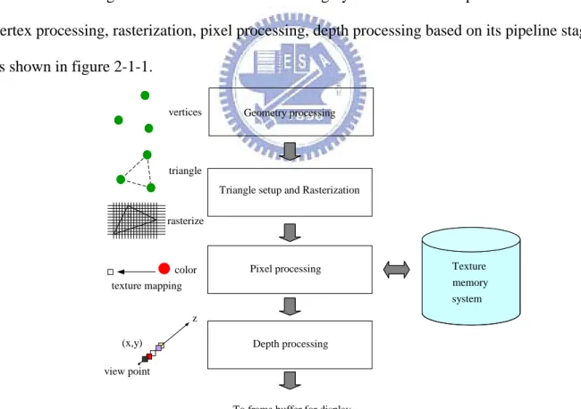
2.1 GPU rendering flow

The rendering flow in current GPU can be roughly divided into four parts which are vertex processing, rasterization, pixel processing, depth processing based on its pipeline stage, as shown in figure 2-1-1.

Geometry processing

Triangle setup and Rasterization

Pixel processing

Depth processing

To frame buffer for display

Texture memory system vertices triangle rasterize color (x,y) z view point texture mapping

Figure 2-1-1 rendering pipeline of GPU

In figure 2-1-1, the vertex processing is done in vertex shaders. The majority works in them is performing vertex’s coordinate translations. These translations actually is a serial of

coordinate translations from vertex’s local coordinate to global environment coordinate and finally translate to view point coordinate.

After vertex processing, the following stage is triangle setup and rasterization. Triangle setup is responsible for assembling primitive according to their view point coordinate. That is finding three vertices which are valid to be assembled into a triangle (primitive). Based on the primitive, rasterization is responsible for interpolating this primitive. In another word, rasterization interpolate each primitive into some fragments. Thus, we obtain the fragments, pixels before output to frame buffer are called fragments.

The pixel processing is done in pixel shaders. Its majority work is coloring each fragment with the texture which is usually stored in the texture memory system, i.e. memory, cache, through the dedicate function units, texture units.

The final processing is depth processing. Since the are many fragments have the same x, y coordinate in the screen but are different in z coordinate, we are target to find out which fragment will not be covered (closest to the view point) and will be final displayed on the screen. Thus, the works in depth processing is simply comparison the depth value (Z value) of each fragment which has the same x, y and pass these fragments to frame buffer for display on the screen.

2.2 The Texture mapping techniques

Texture mapping technique usually invokes multiple textures or MIP maps as samples and also invokes the other techniques, such as bilinear interpolations or trilinear interpolations to produce different amounts of realism. Moreover, the major process of the whole texture mapping is done in special function units in the stage of pixel processing, called texture unit. We will introduce them respectively as following organization:

In section 2.2.1, we will first give an overview of texture data structure.

texture unit which is responsible for coloring the fragment. And it contains coordinate generation, address translation, texels look up and texture filtering.

2.2.1 The textures

Texture is simply a data structure which is used as color reference in pixel shader and can be viewed as a picture or bitmap image. Its dimensions are usually restricted to power of 2 for hardware implementation. Moreover, the width and the height of the texture can be different [4].

A pixel of a texture, call a texel, is a basic cell of a texture and is usually made up of four components, which is R (Red), G (Green), B (Blue), A (Alpha) respectively. And each component is usually one byte width. However, with the High Dynamic Range (HDR) introduced in DirectX 10, a texels can be up to 16 bytes, which each component is up to 4 bytes for more precision

Textures are usually stored in the off-chip large texture memory and on-chip fast texture cache for quickly retrieval in GPU. When the pixel shader needs to paint the fragment, it needs the color information in the textures, thus goes to the texture storage to get the required texels for that fragment.

2.2.2 Texture mapping process flow within Texture Unit

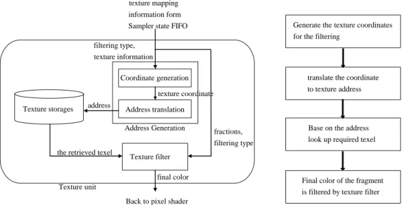
Texture mapping is done within the texture unit. The texture unit is usually in the Pixel shader, since it is responsible for color the fragment according to the filtering type. The processing flow can be roughly classified into four operations, as shown in figure 2-2-2-1.

From Sampler State FIFO [14], we know the required information of how to color the fragment. The information may contain texture filtering type, texture coordinates, base texture address of the required texture, etc.

texture mapping information form Sampler state FIFO

Address Generation

Texture filter Texture storages

Back to pixel shader address final color Coordinate generation Address translation texture coordinate fractions, filtering type Texture unit filtering type, texture information

the retrieved texel

translate the coordinate to texture address

Base on the address look up required texel

Final color of the fragment is filtered by texture filter Generate the texture coordinates for the filtering

processing flow

Figure 2-2-2-1 the texture unit and texture mapping processing flow

After we have the information, the coordinate generator will generate the required texture coordinates based on the filtering type. These texture coordinates may be further translated into texture addresses by the following address translation unit. These translated addresses will be used to look up the required texel in the texture cache next to the texture unit. The texture cache is a fast SRAM storage space, it store the texels information, and can be any traditional cache configuration. After we have retrieved the required texels, we can perform the texture filtering algorithm based on the filtering type, texels, and other information in the texture filter. The final color will be sent back to the pixel shader.

In current high-end graphic card, there are multiple texture units in the pixel shader for performance issue [11]. Moreover, most of the texture units also have multiple texture address units and texture filters which allow processing more filtering algorithms or more complicated filtering algorithm in parallelism [11]. Texture units are allowed to generate the final color of filtering algorithm per cycle.

As mentioned in chapter one, we are target to save average texels access time of filtering. The average texels access time may contain the time spending on coordinate generation, address translation and cache look up.

2.2.2.1 Address translation

In GPU processor, the texel is indexed through texture coordinates, i.e. u, v, coordinates, But in texture memory system, texture is indexed through texture memory address. Since the indexing methods are different between GPU processor and memory system;, thus we need a special function unit which is target to perform the address translation, as shown in figure 2-2-2-1-1.

Indexing in pixel shader 2m w= 2n h= u

v

Indexing in texture memory Base

Figure 2-2-2-1-1 the concept of address translation.

The address translation could be viewed as a translation function with texture coordinates (i.e. u, v), texture dimensions, base address of texture as input and generate the translated address as output [4].

Thus, the complexity of address translation may relate to the texture placement algorithm. If the placement is well design, the address translation could be easy to translate. If not, the address translation complexity could be complicated.

2.2.2.2 Texture filtering

Texture filtering is the method used to obtain the color for a fragment by using the colors of nearby texels in some texture. In another words, it is an attempt to find a value at some point by giving a set of discrete samples at nearby points. Thus, texture filtering is a kind of process that for any given fragment, it goes to loop up some required texels, and calculated the final color for that fragment.

Since one fragment may not usually correspond exactly to one texel, there can be different types of correspondence between a fragment and the texel/texels depend on the position of the textured surface relative to the viewer.

For example, one fragment is exactly the same as one texel of the texture, that is one to one mapping. Closer than that, the texels are larger than fragments. Texels are needed to be scaled up appropriately, known as texture magnification. Farther away, each texel is smaller than a fragment, that is one to many. In this case an appropriate color has to be picked based on the covered texels, via texture minification.

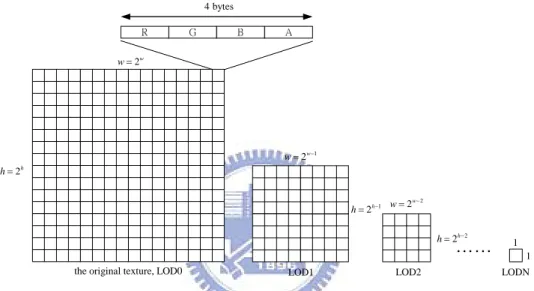
Because the different correspondence between fragments and texels mentioned before, that may necessitate reading all of entire texels and combining their values to correctly determine the fragment color. This process would be a potentially expensive operation. Mipmapping technique is introduced in [12]. It can avoid this by pre-calculating, recursively sampling the texture and storing it in a quarter down to a single texels. As the textured surface moves farther away, the texture being applied switches to the pre-sampled size. Different sizes of the mipmap are referred to as 'levels', with Level 0 being the largest size (used closest to the viewer), and increasing levels used at increasing distances. As shown in figure 2-2-2-2-1, we have an example of how the mipmaps looks like.

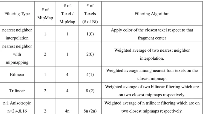
The filtering method can be roughly classified according to the image quality and computation complexity.

method - it is only look up the closest texels’ color for the mapped fragment. While fast, this results in a large number of artifacts, thus image quality is the worst.

The second one is nearest neighbor with mipmapping. According to the fragment’s Z value, we select the two closest mipmaps first. For each mipmap, by applying Nearest neighbor interpolation, we got two selected texels. Finally, the final color for that fragment is the result of weighted average of those two texels. This reduces the aliasing and shimmering significantly, but does not help with blockiness.

4 bytes

the original texture, LOD0 2w w= 2h h= 1 2w w= − 1 2h h 2 2w w − − = LOD1 = 2 2h h= − LOD2 1 1 LODN

Figure 2-2-2-2-1 the mipmaps and data structure of a texel

The third on is bilinear filtering. In this method the four closest texels on a nearest mipmap level to the fragment center are chosen, and final color for that fragment is the color of weighted average among them. Figure 2-2-2-2-2 shows the concept of bilinear filtering algorithm. Bilinear filtering is almost invariably used with mipmapping; though it can be used without, it would suffer the same aliasing problems as nearest neighbor. Moreover, bilinear filtering is the basic component of the following filtering method. And they can be viewed as several pieces of bilinear filtering

T1 T2 T3 T4 f1 1 f 2 f

final filtered color the 4 required texels of a bilinear filtering

the mapped fragment 1 f 2 f

Figure 2-2-2-2-2 the concept of bilinear filtering

The fourth one is trilinear filtering. It can be treated as a weighted average of two pieces of bilinear filtering. For each of two closest mipmap levels, perform the bilinear filtering. And the final color for that mapped fragment is the color which is the weighted average of the two bilinear filtering results. Of course, closer than Level 0 there is only one mipmap level available, and the algorithm reverts to bilinear filtering.

The final one is anisotropic filtering. It is the highest quality filtering available in current consumer 3D graphics cards. If we need to color a plane which is at an oblique angle to the camera, bilinear or trilinear filtering would give us insufficient horizontal resolution and extraneous vertical resolution. Anisotropic is a method of enhancing the image quality of textures on surfaces that are far away and steeply angled with respect to the camera. The final color of that mapped fragment is the color which is the “trilinearly” average of the n pieces of trilinear filtering results. The value n called anisotropic ratio, horizontal direction to vertical direction, is defined by application.

Filtering Type # of MipMap # of Texel / MipMap # of Texels (# of Bi) Filtering Algorithm nearest neighbor interpolation 1 1 1(0)

Apply color of the closest texel respect to that fragment center

nearest neighbor with mipmapping

2 1 2(0) Weighted average of two nearest neighbor interpolation.

Bilinear 1 4 4(1) Weighted average among nearest four texels on the closest mipmap.

Trilinear 2 4 8 (2) Weighted average of two bilinear filtering which are on two closest mipmaps respectively. n:1 Anisotropic

n=2,4,8,16 2 4n 8n (2n)

Weighted average of n trilinear filtering which are on two closest mipmaps respectively.

2.3 Related Research

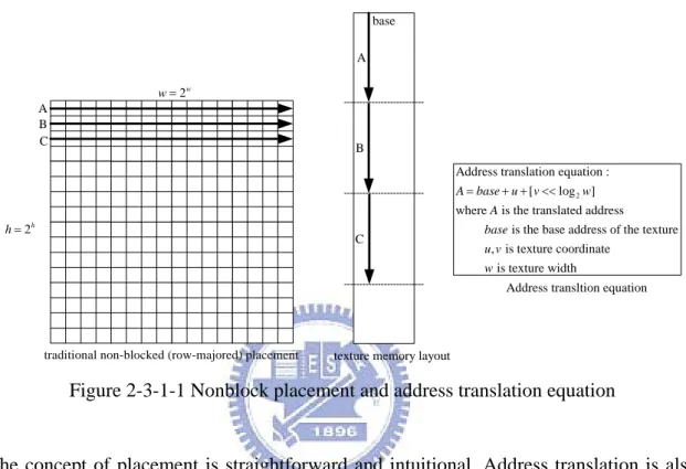
2.3.1 Nonblock placement

Traditionally, texture is placed in the texture memory by using row-major concept, as shown in figure in 2-3-1-1. This is also known as Nonblock placement.

traditional non-blocked (row-majored) placement 2w w= 2h h= base A B C A C B 2

Address translation equation : [ log ] where is the translated address is the base address of the texture , is texture coordinate is texture width A base u v w A base u v w = + + <<

Address transltion equation

texture memory layout

Figure 2-3-1-1 Nonblock placement and address translation equation

The concept of placement is straightforward and intuitional. Address translation is also straightforward. However, since texture filtering have spatial locality, that is the required texels of a bilinear filtering is in a 2 by 2 region, and the required texels of next bilinear filtering is usually closed to the current one, Nonblock placement could be considered as a non-efficiency placement due to the long texture’s width and always row-major.

Among these four required texels, the upper and lower two will in two adjacent rows respectively, as shown in figure 2-3-1-2. However, if the row of texture is very long, the required texels will be separated far away in the texture memory.

Moreover; when the cache line size is smaller or equal to the size of a single row data structure, the required texels which are in two adjacent rows will be placed in two different cache lines. Thus the upper/lower two required texels will be in different cache lines and for

A texture

row-major

The required texels of a bilinear filtering are in two adjacent rows

Figure 2-3-1-2 access condition of Nonblock placements

2.3.2 4D placement

texture memory layout Base

2 2

Address translation equation :

= [ log ( )]

[ log ( )] where , the base address of the texture is texture width

Tile address base bv w bw bu bw bw base w + << ∗ + << ∗ 2 2 is texture height , is texture coordinate , is tile coordinate = log = log h u v bu bv bu u bw bv v bw >> >> 2 = & ( 1) = & ( 1) = [ log ( )]

where is translated address

, is sub coordinate within a tile i su u bw sv v bw A Tile address su sv bw A su sv bw − − + + << s tile width w2 2 A 2 * 2 tileh

One level tile based (4D) placement

1 2 2w w w= + 1 2 2h h h= + 2 2w w= 2 2h h= A texel

Address translation equation

Figure 2-3-2-1 4D placement and address translation equation

4D placement [4] is also known as tile-based placement, as shown in figure 2-3-2-1. The concept of 4D placement is row-majored and one level tile-based: original texture is divided into some squared tiles and inter/intra-tile is row-major.

Since texture filtering has spatial locality, the placement which place the texels in a form of group could get better cache performance. This is because the required texels of a filtering may be fall into a 4D tile and they are placed in the texture memory nearby according to the tile size.

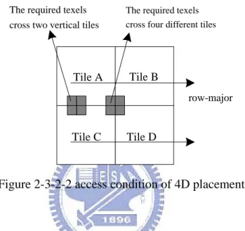
However, since inter-tile is also the row-major, the required four texels of bilinear filtering will have strongly chances to cross two adjacent tiles in the column or four different

row-major

The required texels cross two vertical tiles

tiles, shown in figure 2-3-2-2. Thus these required texels may be placed separately in texture memory and may introduced conflict miss in direct mapping cache. In [4], they say when the size which is texture width multiplies tile width is multiple of cache size and cache line size is multiple of tile size, conflict misses will occur due to the upper and lower tile will have the same cache index number. By padding the unused tile to form another new column, the problem can be solved. However, texture memory spaces will waste.

Tile B

Tile C Tile D Tile A

The required texels cross four different tiles

Figure 2-3-2-2 access condition of 4D placement

Moreover, if cache line size is equal to the tile size, for those four requited texels in the same cache line, they are two and two continuous or all continuous due to 4*4 tile size. If two texels are in the same cache line, they are continuous like Nonblock placement or discontinuous due to the two texels are placed on different rows in the tile.

The address translation of 4D placement proposed in [4] invokes many arithmetic operations, such as ADD operation. Due to texture address is 32-bits or 64-bits [4] in current GPU architecture, the ADD operation may have long carry propagation according to the hardware implementation. Thus, the propagation could be the critical path of the address translation.

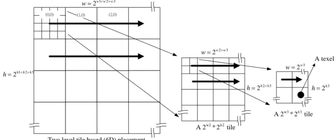
2.3.3 6D placement

w2 2

A 2 * 2 tileh Two level tile based (6D) placement

1 2 3 2w w w w= + + 1 2 3 2h h h h= + + 2 3 2w w w= + 2 3 2h h h= + 3 2w w= 3 2h h= A texel w3 3 A 2 * 2 tileh

Figure 2-3-3-1 the related work of 6D placement

6D placement [4] is known as two-level tile-based placement, as shown in figure 2-3-3-1. The original texture is divided into some squared larger tiles and inter-larger tile is row majored. Within a larger tile, 4D placement is applied to it.

The placement is proposed to improve the conflict miss which occurs in 4D placement. Unlike the padding unused tiles to form a new column, 6D placement will not waste the memory space. However, the address translation idea proposed in [4] is still following the concept of 4D placement. It invokes arithmetic operations, such as ADD operation.

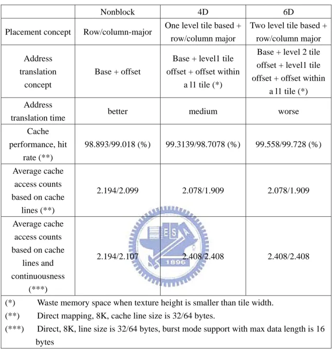
Finally, we have a table 2-1 to summarize the three placement algorithms in term of address translation time, cache hit rate, average cache access counts based on cache lines and average cache access counts based on cache lines and continuousness. We expect the address translation time of Nonblock is better than 6D placement. The cache hit rate of 6D is better than Nonblock placement. Average cache access counts based on cache lines of 6D/4D placement is better than Nonblock placement. Finally, average time of cache access based on cache lines and continuousness of 6D/4D placement is better than Nonblock placement.

Nonblock 4D 6D Placement concept Row/column-major One level tile based +

row/column major

Two level tile based + row/column major Address

translation concept

Base + offset

Base + level1 tile offset + offset within

a l1 tile (*)

Base + level 2 tile offset + level1 tile offset + offset within

a l1 tile (*) Address

translation time better medium worse

Cache performance, hit rate (**) 98.893/99.018 (%) 99.3139/98.7078 (%) 99.558/99.728 (%) Average cache access counts based on cache lines (**) 2.194/2.099 2.078/1.909 2.078/1.909 Average cache access counts based on cache lines and continuousness (***) 2.194/2.107 2.408/2.408 2.408/2.408

(*) Waste memory space when texture height is smaller than tile width. (**) Direct mapping, 8K, cache line size is 32/64 bytes.

(***) Direct, 8K, line size is 32/64 bytes, burst mode support with max data length is 16 bytes

Chapter 3 Design

3.1 Design Overview

Our design can be roughly divided into two topics: the first one is focus on the new placement algorithm that is how to place the texture in the texture memory. The second one is focus on the possible texture cache supports in the GPU.

In the placement topic, motivated by the related work proposed in [4], we will propose the new texture placement algorithm by using the recursive concept. The new placement is called Recursive Z placement, and can be viewed as multi-level row-major placement which is extended from 4D/6D placement. Later on, we will try to further improve the RZ placement in term of the continuousness of required texels with in a cache line. We have two main ideas. The first one is motivated from shape. We can try another shape instead of Z shape. The other is motivated from tile size. We can try larger base tile size instead of 2*2 to gain more continuousness.

After we have the placement, we should develop the address translation idea of these placements. The idea should be easy. And the logic should also easy to implement. It may use bit-wise logic operations to accomplish the translation.

In the possible texture cache support topic, we list three possible texture cache supports in current GPU architecture which are baseline texture cache support, texture cache support1 and texture cache support2. The baseline texture cache support and texture cache support 1 are common in current texture cache. And our design is focus on texture cache support 2 which can retrieve the required texels of bilinear filtering in the same cache line.

3.2 Texture placement

In the section, we will design the new placement algorithm. That is how to place the texture in the texture memory. The new placement algorithm will be design in three aspects which are cache hit rate, average cache access counts and address translation time. Finally, we will propose a possible logic implementation for the address translation idea.

3.2.1 Recursive Z placement (RZ)

Our new placement is called Recursive Z placement. The placement strategy is placing the texel in the recursive z scan line, as shown in figure 3-2-1-1. In the term of iteration, we have the base case (1*1) which only invokes one texel. The next case (2*2) is iteratively integrated with the four previous cases by using Z shape placement Recursive Z can also be viewed as multi-level row-major placement which is extended from 4D/6D placement proposed in [4].

Figure 3-2-1-1 recursive z placement

Since the required texels of bilinear filtering has spatial locality, that is bilinear filtering itself is a form of 2*2 region and the required texels of current bilinear filtering is close to the next one, tile-based placement can avoid placing texels continuously along one u/v direction, i.e. row-major/column-major, like Nonblock placement. Thus, the required texels of filtering may not be separated far away.

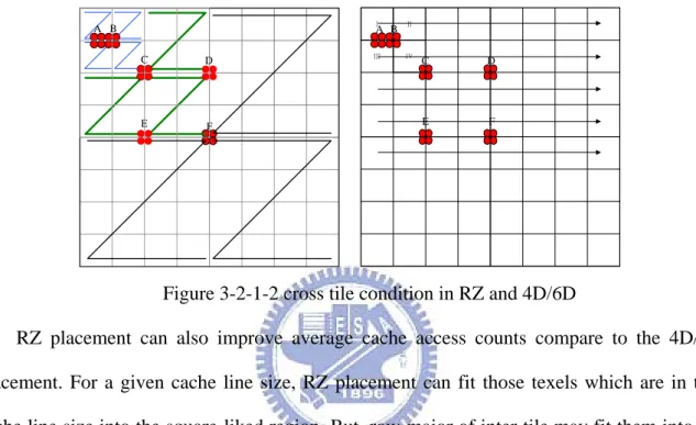
3-2-1-2, the required texels of filtering can be cross two/four tiles/Z in RZ/4D/6D. If we have four required texels, say A, RZ can place them more closely than inter-tile is row-major (4D/6D). B, C is the same, too. However, if we have D/E/F, RZ may be worse than 4D/6D placement. But, as mention before, filtering have spatial locality. We expect RZ placement have better cache performance in average.

A B C D F E A B C D E F

Figure 3-2-1-2 cross tile condition in RZ and 4D/6D

RZ placement can also improve average cache access counts compare to the 4D/6D placement. For a given cache line size, RZ placement can fit those texels which are in that cache line size into the square-liked region. But, row-major of inter-tile may fit them into the rectangular-liked region. In figure 3-2-1-3, if we have cache line size is cable of 4 tiles/Z, we will not cross another cache line when access A or B texels in RZ placement. But, it may will in 4D/6D placement.

A B

C D

E F

3.2.2 Different placement policies

Under some texture cache system with burst mode technology support, texture cache support1, it may retrieve the required texels of bilinear filtering in one cache access if they are all continuous. It can be done by sending the start address of the required texels and the data offset for the required texels in continuousness. If they are discontinuous, the cache may not retrieve them in one cache access. Thus, the consideration of continuousness is also important.

3.2.2.1 Recursive Z with U (RZU)

Although the required four texels within a base 2*2 Z-shape and 2*2 u-shape are all continuousness, if the required texels are crossing two z or two u in horizontal/vertical, U-shape could be potentially have more benefits than z-shape. This is because the U shape has three directions of continuousness benefits. But the z-shape only has two. Thus, we may change the z-shape to the u-shape.

0 3 1 2 4 6 5 7 8 11 9 10 12 14 13 15

Figure 3-2-2-1-1 Recursive Z with U placement

RZU placement is obtained by changing the 2*2 Z-shape to 2*2 u-shape as shown in figure 3-2-2-1-1. And the placement policy between 2*2 tile is the same as RZ placement. It is also the multi-level tile-based like RZ placement. Thus, we expect the cache hit rate is equal to RZ placement under three kinds of cache support.

discontinuous. But, in average, we may improve the average cache access counts under texture cache support 1. However, the average cache access counts may equal to RZ in texture cache support 2.

3.2.2.2 Recursive Z with Flipped-U (RZFU)

We can further improve the RZU by flipping the lower U over in order to have the bottom of the upper and lower U edge to edge, as shown as red circle in figure 3-2-2-2-1. However, we may have texels covered by blue circle discontinuous as shown in figure 3-2-2-2-1. And we can also try to flip the upper two U over as shown in figure 3-2-2-2-2. However, by doing this, we may have some required texels discontinuous.

Figure 3-2-2-2-1 Recursive Z with Flipped-U v1

1 2 0 3 5 6 4 7 8 11 9 10 12 15 13 14

Figure 3-2-2-2-2 Recursive Z with Flipped-U v2

RZFU1/2 placement can also be viewed as the multi-level tile-based like RZ placement. Thus, we expect the cache hit rate is equal to RZ placement under three kinds of cache support. Whether the average cache access counts under texture cache support 1 of RZFU1 is better than RZFU2 may dependent on the probability. If the required four texels are always

happen to red circle in figure 3-2-2-2-1, the RZFU1 could be better. If the required four texels are always happen to blue circle in figure 3-2-2-2-2, the RZFU2 could be better. The average cache access counts may equal to RZ in texture cache support 2.

3.2.2.3 Recursive Z with Snake (RZS)

In section of 3-2-2-1 and 3-2-2-2, we improve the RZ placement by changing z-shape to u-shape. In this section, we improve the RZ placement by changing base 2*2 tile size to larger n*n tile size. We found that the larger tile size we choose, the probability of required four texels of bilinear filtering crossing two/four tiles is lower. If the required four texels of bilinear filtering cross two/four tiles, the discontinuous may occur. Another reason for larger tile size is that we have more placement policy within the larger tile size.

We propose a new placement, called Recursive Z with snake. The snaked-tile can be viewed as row-major instead the direction of odd row and we take 4*4 snaked tile size as example shown in figure 3-2-2-3-1. And the placement policy between 4*4 snaked-tile is also the same as RZ placement.

Figure 3-2-2-3-1 Recursive Z with Snake placement

However, we can not increase our base tile size unlimited. The larger snaked tile size we have, the placement within that tile is more like Nonblock placement. The spatial locality of required four texels of bilinear filtering may decrease. Thus, it may affect cache hit rate.

3.2.3 Address translation idea of RZ

The address translation can be viewed as a translation function with inputs, and generates the output,

, , , ,

m n U V B A , which are dimension of texture’s width and

texture’s height, u coordinate, v coordinate, base address of the texture and the translated address as defined in figure 3-2-2-1. So, we are going to find a RZ function which is

( , , , , ) A=RZ m n U V B Texture's width is 2 2 , , Texture's height is 2 2 , The u-coordinate is , 0 The v-coordinate is , 0 The translated address is 2 The base address of texture is 2

m d n d s s Wn m d N Hn n N U U Wn V V Hn A B = ≤ ∈ = ≤ ∈ ≤ ≤ ≤ ≤ ≤ ≤

Figure 3-2-2-1 definition of terms

There are three cases in RZ, which are m equal to n, m smaller than n, and m larger than n, respectively. However, the main concept of these cases is the same, that is recursive translation.

The first case is m equal to n, that is texture’s width is equal to texture’s height. As shown in Figure 3-2-2-2, the base case only invokes one texel, and the translated address

. A is 0 0 A= A=a a1 0=v u0 0 0 u 0 v 0 1 0 1 3 2 1 0 1 1 0 0 A=a a a a =v u v u 1 0 u u 1 0 v v _{00 01 10 11} 00 01 10 11 1 0 0 0 a a =v u 0 u 0 v _{0 1 0 1} 0 1 0 1 3 2 1 1 a a =v u 1 u 1 v _{0 0 1 1} 0 0 1 1

Base case iteration I iteration II Least significant 2 bits Most significant 2 bits

Figure 3-2-2-2 the case I of address translation

0

v

1 0

a a could be v u_{0 0}, which u₀and are the least significant bit of U and V, respectively. In iteration II, we first focus on the least significant 2 bits of each translated address. And we found that each of the bit pattern in dotted rectangle is corresponding to the bit patterns found in the iteration I. Thus, we can suggest that the least significant 2 bits of translated address in iteration II may equal the bit pattern in iteration I, that is v u_{0 0}.

We now look at the most significant 2 bits of each translated address. And we can also use Karnaugh Map to translate a a_{3 2}. The result shows that a a_{3 2}=v u_{1 1}. So the translated

address of iteration II, .The bit pattern can be view as the form which is iteratively cross interleaving each u and v coordinate bit, respectively. In the term of recursive concept, the translated address bit pattern of base case is the subset in iteration I. And the translated address bit pattern of iteration I is also the subset in the iteration II, iteration II is the subset in iteration III, etc.

3 2 1 0 is 1 1 0 0

a a a a v u v u

Now, we can suppose that when the texture is 8 by 8, the translated address

is by cross interleaving each least significant 3 bits of u and v coordinate.

5 4 3 2 1 0 a a a a a a 2 2 1 1 0 0 v u v u v u 2 2 Example: (3,3, 4,7, ) 3 4 100 7 111 Rz B m n U V = = = = = = U V = = ' A =1 1 1 0 1 0 1 0 0 1 1 1 4 7 = = ( ' 2) A= A << +B

Figure 3-2-2-3 example of address translation case I.

For example, since we are going to translate the pair of (4, 7), all we need to do is cross interleaving each least significant 3 bits of u and v coordinate, respectively. In figure 3-2-2-3, the result of cross interleaving is 58.

However, texture filtering may sample the texture with n by m dimension which is not equal , but is power of 2, respectively. The translation idea mentioned before may need to

modify slightly. In figure 3-2-2-4, the texture’s width is larger than texture’s height. This is . In the case, since texture’s height is shorter than texture’s width, for any texel, we do not have enough v-coordinate bits to cross interleave with u-coordinate bits. On the other words, after perform cross interleaving, some u-coordinate bits are left. These left bits should be followed by the cross interleaved result, in order to obtain the correct translated address.

m>n 0010 3 2 1 0 2 1 0 0 A=a a a a =u u v u 0011 1000 1001 2 1 0 u u u 0 v _{000 001} 0000 0001 0101 0111 1101 1010 1011 0100 1100 0110 1110 1111 010 011 0 1 iteration II 100 101 110 111 0 0 A= 00 1 0 0 0 A=a a =v u 01 10 11 0 u 0 v 0 1 0 1

Base case iteration I

10 1 0 0 0 a a =v u 11 00 01 0 u 0 v _{0 1} 00 01 01 11 01 10 11 11 00 10 00 10 0 1 0 1 0 1 0 1

Least significant 2 bits

00 3 2 2 1 a a a=u u 00 10 10 2 1 u u 00 00 00 00 01 01 11 10 10 01 11 01 11 11 01 01 10 10 11 11

Most significant 2 bits

Figure 3-2-2-4 the case II of address translation

In figure 3-2-2-4, we have 3 u-coordinate bits and 1 v-coordinate bit to cross interleave for translated address. After cross interleaving, we have a part of translated address

equal to . However, the translated address should have four bits to index the required

texel. The part of address, , we do not assign them yet. So, we focus on the most significant 2 bits of the translated address. The bit pattern of each texel is exactly the same as the unused 2 u-coordinate bits, .

1 0 a a 0 0 v u 3 2 a a 2 1 u u

U V = = ' A =1 01 0 11 9 3 = = ( ' 2) A= A << +B 10 0 1 1 1 2 2 Example: (4, 2,9,3, ) 9 1001 3 0011 Rz B m n U V > = = = =

Figure 3-2-2-5 example of address translation case II

For example, since we are going to translate the pair of (9, 3) and m is larger than n, we should need to cross interleave 2 bits of u and v, respectively. And the left 2 bits, , should be followed by the cross interleaved result. In figure 3-2-2-5, the result of cross interleaving is 43.

3 2

u u

The conclusion is that, when the texture’s dimension is not equal, the cross interleaving is still work, but the remaining coordinate bits should be followed by the cross interleaved result. In this case, the two bits should be followed by the cross interleaved result in order to obtain the correct translated address.

Moreover, in terms of recursive concept, the inequality of two dimensions means incompletely recursive texture. The iteration of placement will break when the short side is met. So, the recursive bit pattern will be limited when the coordinate bits of shorter side is exhausted.

The final case is shown in figure 3-2-2-6. That is texture’s width is smaller than texture’s height. After we cross interleave them, the left v-coordinate bits, , should be followed by

the cross interleaved result, say , in order to obtain the correct translated address.

2 1

v v

0 0

0 A= A=a a1 0=v u0 0 0 u 0 v 0 1 0 1

Base case iteration I

3 2 1 0 2 1 0 0 A=a a a a =v v v u iteration II 0 u 2 1 0 v v v _{0 1} 000 001 010 011 100 101 110 111 2 1 0 v v v 00 00 01 01 10 10 11 11 0 u 0 v _{0 1} 0 1 0 1 0 1 0 1 1 0 0 0 a a =v u a a3 2=v v2 1

Least significant 2 bits Most significant 2 bits

Figure 3-2-2-6 the case III of address translation

2 2 Example: (2,4,3,9, ) 3 11 9 1001 Rz B m n U V < = = = = V U = = ' A =1 001 11 9 3 = = ( ' 2) A= A << +B 1 00 1 1 1

Figure 3-2-2-7 example of address translation case III

For example, since we are going to translate the pair of (3, 9) and m is larger than n, we should need to cross interleave 2 bits of u and v, respectively. And the left 2 bits, , should be followed by the cross interleaved result. In figure 3-2-2-7, the result of cross interleaving is 39.

3 2

v v

So far as here, the translated address mentioned before is not the final address we are going to use. This is because we did not take base address of the texture as a consideration. So the translated address will be added with base address and be left shifted 2 bits for 4 bytes a texel. Final address is( 'A <<2)+B

cases.

1 1 2 2 1 1 0 0

1 2 1 1 1 1 1 0 0

1 2 1 1 1 1 1 0

Address translation of Recursive Z :

case I ( , ) ' case II ( , ) ' case III ( , ) ' r r r r m m m m n n n n n n m m Wn Hn m n r A v u v u v u v u Wn Hn m n A u u u u v u v u v u Wn Hn m n A v v v v v u v u v − − − − − − + − − − − + − − = = = = > > = < < = 0

Final address ( ' 2) , for one texel is 4 bytes Thus we have address translation function ( , , , , )

u

A A B

A Rz m n U V B

= << +

=

Figure 3-2-2-8 summary of RZ address translation function

3.2.4 Address translation of other placements

Since the inter-tile placement policy of RZU, RZFU1/2 and RZS is identical to the Recursive Z placement, the difference of address translation among these placements could be the least significant bits. We summarize a table to list the difference of translated address bit pattern among these placements.

Recursive Z Recursive Z with U

3 a 2 a 0 a 1 a 0 u 0 v 1 u 1 v

Recursive Z with Snake

0 u 0 0 v ⊕u 1 u 1 v 0 1 v ⊕u 0 0 v ⊕u 0 v 1 v

Recursive Z with Flipped U 1/2

0 u 0 0 1 0 0 1 u ⊕ ⊕v v u ⊕ ⊕v v 1 u 1 v

Table 3-2-4-1 Summary of least significant four bits of address among placements

3.2.5 Address translation logic implementation

address. In [4], the address translation time of Nonblock and 4D and 6D may take long time to translate, since they may invoke arithmetic operations, such add operation, and the propagation path in add operation may up to 32 bits or 64 bits, due to texture address is 32 bits of 64 bits and hardware implementation of Adder. We are going to use bit-wise logic operations to translate the address, Since there is the regularity in the Recursive Z. And we expect that the address translation time is short.

In the pervious section, no matter what translation case it is, the translated address can be viewed as combination of common address field and differential address field, as shown in figure 3-2-5-1. The common field only invokes the bit pattern which is cross interleaved form some bit toggles of U and V coordinate. And the Differential field invokes only U or V coordinates or simply zero. The combination invokes bit-wise OR operations.

1 1 1 1 0 0 1 1 1 1 0 0 1 2 1 differential field : 0 common field : differential field : 0 common field : 0 r r r r m m n n v u v u v u v u v u v u u u u u − − − − − − + 1 1 1 1 0 0 1 2 1 1 1 1 1 0 0 1 2 1 1 1 1 1 0 differential field : 0 common field : 0 n n m m n n n n n n m m m m v u v u v u u u u u v u v u v u u u u u v u v u v u − − − − + − − − − + − − 0 1 2 1 1 1 1 1 0 0 un−un− um+u vm m−um− v u v u Bit-wise OR Bit-wise OR Case I (m= =n r) Case III (m<n) Case II (m>n) Bit-wise OR

Figure 3-2-5-1 concept of address translation unit

The address translation unit can be roughly divided into three parts based on the concept of combination mentioned in figure 3-2-5-1, which are common field generator, differential field generator and additional operations as shown in figure 3-2-5-2.

' A the translated address coordinate and other information

Figure 3-2-5-2 global view of address translation logic

Common field generator is responsible for the generation of the bit pattern by cross interleaving some bit toggles of each coordinate. Differential field generator is responsible for the generation of the bit pattern by concatenating the bit toggles which are not cross interleaved. The obtained two filed are then combined by bit-wise OR operations. Finally, the additional operations are responsible for left shift and add the base address.

In common field generator, what we concern about is how many least significant bit toggles of each U, V coordinate should we cross interleave? Intuitively, by comparing m with n and choosing the smaller one, we have the number of bit toggles that should be cross interleaved of each coordinate. For example, if m=7 and n=3, there are three least significant bit toggles of each coordinate we should cross interleave. As a result, the common field generator could have a compare and select logic as shown in figure 3-2-5-3 and a flexible cross interleaving logic which can perform cross interleaving operation under any number of least significant bit toggles.

Comparator ?1:0 m≥n m n 4 4 4 4 m n 0 1 mux 4

Figure 3-2-5-3 compare and select logic

The compare and select logic is the comparator combined with a 2 to 1 mux. The logic can tell us the smaller one, say m or n. Thus, we know how many bit toggles we should cross

0 0

implemented in a form of mux. However, the mux can be the critical path in common field generator. How about use the concept of integration by smaller and unique cell to implement the common field generator? If we can design a cell which can cross interleave the two inputs, one bit toggle from U and the other from V, by a control signal, we can concatenate many of them of form our the common field generator.

The control signal for each cell is generated through an encoder which can encode the output from compare and select logic, i.e. if we have the output form compare and select logic, say 3, that is we should cross interleave least significant three bits form U and V, thus the encoder will generate the enable bit pattern, . Based on the enable bit pattern, we should

cross interleave from each significant three bit toggles of U and V, i.e. and .

2 111 2 u ∼u v₂ ∼v n

u

v

c

Figure 3-2-5-3 one cell of common field generator

Figure 3-2-5-3 represents the one cell of common field generator. The control signal, , is from the corresponding bit position in enable bit pattern. Figure 3-2-3-4 shows the common field generator which is obtained by integrating n cells.

Ei 0 c 1 c 0 u 0 v 2 c 3 c 1 u 1 v 2n 4 c ₋ 2n 3 c − 1 n u− 1 n v− 2n 2 c ₋ 2n 1 c − n u n v n E En−1 E1 E0 cross interleave

The differential field generator is responsible for generation the differential field of the translated address under any given m and n. For example, if we have m=7 and n=3, the differential field can be obtained by setting bit toggles to zero and left shifting 3 bits,

like .

2 1 0

u u u

5 4 3000000

u u u

So what we concern about is the differential field is from most significant bit toggles of U or V and How many bit toggles will be used and their bit position? Since we have known who the smaller one is(m or n), by using the result, we can select the desired coordinate

. And we also have the enable bit pattern generated from the encoder.

(m≥n?U:V)

Thus, we can use the information to generate the differential field. In figure 3-2-5-5, the comparison result is used to select the desired coordinate (U or V) by using another 2 to 1 mux. After that the selected result, say A and the result from enable encoder, say B, is passed to the Bit filter. It can set the unnecessary bit field of Bto zero. Finally, the left shifter can left shift any number of bit of B' based on the smaller one value of m or n .

enable encoder 16 16 v u 0 1 4 4 m n 0 1

mux Bit filter

B&(~A) 16 32 differential field B A exten c to 32 bits and left shift bitsx

x 4 16 16 c Comparator ?1:0 m≥n m n 4 4 mux 4

Figure 3-2-5-5 differential field generator

For example, if we still have m=7 and n=3, the input A, B to the bit filter is coordinate U and bit pattern form enable encoder. The bit filter will filter out the least three

significant bit of coordinate U. the left shift will left shift 3 bits based on the pattern .

2

111

2

3.3 Three possible texture cache supports

Although, the average texels access time of bilinear filtering is affected by the texture placement, it is also affected by the hardware design (texture unit/texture cache). We have three possible texture cache supports in different hardware cost. And each of them has different texels retrieval capability.

3.3.1 Baseline texture cache support

The baseline texture cache support is straightforward. The texture cache can retrieve one required texel data with a address request. In this kind of system, only the address translation time and texture cache miss rate will affect the average texels access time of bilinear filtering. This is because every address request can only retrieve one texel data to the texture filter. Thus, average cache access counts of bilinear filtering are always four.

3.3.2 Texture cache support 1

The texture cache support 1 is a common texture cache with burst mode support. The burst mode technique is done by sending a start address and the maximum required data offset; the receiver can get the required data as soon as possible. Since the required texels of bilinear filtering are four, the maximum data offset length is 16 bytes. In the other words, if the required texels are adjacent to each other within a cache line, the cache can retrieve all of the required texels in one cache access. Under the texture cache support, the average cache access counts may affected by whether the required four texels are adjacent to each other.

3.3.3 Texture cache support 2

Since the required texels of bilinear filtering could be potentially in the same cache line, for those texels in the same cache line, we can retrieve them in one cache access no matter whether they are continuous or not. This kind of texture cache support is more flexible than the previous one. Thus, we can retrieve more required texels in one cache access. However, for those texels are not in the current been accessed cache line, we still have another cache

access to get them.

3.3.3.1 Possible design of texture cache support2

Base on the concept mentioned in 3.3.3, we need case identifier, texels router and the modified coordinate generator to accomplish the task.(Shown in figure 3-3-3-1-1) Each of them is describe in the following sections.

n n (A,case#, LSB[u ],LSB[v ]) 1 1 (m,n,u ,v ,B) case # Texture unit coordinate generator cases identifier texture filter n n (m,n,u ,v ,B) Address translation unit 1 1 (u ,v ) Texture cache c a c h e lin e b u ffe r address low order bits of coordinate and case #

mux1 mux2 mux3 mux4

2-4 decoder E1E2E3E4 offset2 offset3 offset4 E1 E2 E3 E4

offset1 offset2 offset3 offset4 case # texel4 texel3 texel2 texel1 offset generator

Figure 3-3-3-1-1 Texture cache support 2

3.3.3.1.1 Case identifier

Since the required texels of bilinear filtering is a form of 2 by 2 texels, these four texels can be potentially in one, two, four cache lines. We can identify the case condition through coordinate , as shown in figure 3-3-3-1-1. In figure 3-3-3-1-1, w supposes that cache line size is 64bytes (16 texels) and the condition can be roughly classified into 4 types.

1 1

( , )u v

Case I is the required texels are fall into a single cache line. Case II is two of the required texels in the row are fall into a cache line, and the other two are fall into another cache line. Case III is two of the required texels in the column are fall into a cache line, and the other two are fall into another cache line. Case IV is four required texels are in different cache lines.

case III case IV

case II

cache line with 16 texels

case I

the required texels of bilinear filtering

1 1

(u ,v ) (u +1,v )1 1

1 1

Figure 3-3-3-1-1-1 multiple cache lines conditions

Since we know the placement algorithm and cache configuration, i.e. RZ placement, cache line size, the case condition can be obtained though identification of coordinate . The identification is easy and straightforward. If we have RZ placement and cache line size is 16 texels, the 16 texels can be shown as the 16 white squares in the figure 3-3-3-1-1-1. We can partition the 16 texels into 4 regions; say A, B, C and D, as shown in figure 3-3-3-1-1-1.

1 1 ( , )u v 1 1 1 1 1 1 f (u %3 0 and v %3 0) case IV else if (u %3 0 and v %3 0) case III else if (u %3 0 and v %3 0) case II else case I i = = = ≠ ≠ = (1,0) (0,0) (0,1) (1,1) (2,0) (3,0) (2,1) (3,1) (0,2) (1,2) (2,2) (3,2) (0,3) (1,3) (2,3) A B (3,3)

assume cache line size is 64 bytes (16 texels)

C D

Figure 3-3-3-1-1-2 operation of case identifier

If the is fall into region A, the other three coordinates will also in the same cache line. Thus it could be case I, all required texels are in the same cache lines. If the is fall into region B, it is the case III, two texels in the column are in the same cache

line, the other two texels are in the other cache line. The worst case is fall into region D; all required texels are in different cache lines.

1 1 ( , )u v 1 1 ( , )u v 1 1 ( , )u v

The identification algorithm is shown in the figure 3-3-3-1-1-2. If both and mod

3 are equal to 0, region D. If but not mod 3 are equal to 0, region B. If not but

mod 3 are equal to 0, region B. If neither nor mod 3 are equal to 0, region A. The mod operation can be implemented through Bit-wise logic AND operation of two lower order bits of coordinate and , i.e. mod 3 is equal to 0 can be implemented through the

1 u v₁ 1 u v₁ u₁ v₁ 1 u v₁ 1 u v₁ u₁

result of AND and is equal to 0. Thus all we need is low order two bits of coordinate

and to identify the case conditions. Since we have total four cases, we can encode the cases by using 2 bits signal. 00 means case I. 01 means case II. 10 means case III. 11means case IV. 1 1 u u₀1 1 u v₁

However, the texture dimension can be any magnitude of power of two. That is the texture height/width can be smaller or equal to 2. In these cases, the 16 texels which are in the cache line will not be square-like region any more in the texture. It could be the rectangular with narrow width or wider height dimension. As a result, the identification algorithm in figure 3-3-3-1-1-2 should be modified. The values A, B which is the magnitude mod A

and mod B in figure 3-3-3-1-1-2 should be changed based on the texture dimension.

1

u

1

v

In the original, the 16 texels are in the 4*4 rectangular, the magnitude of A should be 3, and B should be 3, as shown in figure 3-3-3-1-1-2. However, if the texels are in a form of 16*1 rectangular, A should be 15, B should be 0. If they are in a form of 1*16 rectangular, A should be 0, A should be 15. If 8*2, A should be 7, B should be 1. If 2*8, A should be 1, A should be 7.

Thus we have the prefix operation which can tell the case identifier what the magnitude of A and B should the identifier use. And there are five cases if cache line size is 64 bytes (16texels). Which are corresponding to 4*4, 8*2, 2*8, 16*1 and 1*16 rectangular. The classification can be done through the m, n which is power of width and height, respectively. By comparing m and n, we know the case and can enable one of the five enable signals. And the enabled case can perform future case identification based on the coordinate . The overview of case identifier can be shown in figure 3-3-3-1-1-3.

1 1

case identifier of 4*4 case identifier of 8*2 case identifier of 16*1 case identifier of 1*16 case identifier of 2*8 enable enable enable enable enable 2 1 0 0 (u u u ,v ) 1 0 1 0 (u u ,v v ) 0 2 1 0 (u ,v v v ) 3 2 1 0 (u u u u ) 3 2 1 0 (v v v v ) enable of 4*4 enable of 8*2 enable of 2*8 enable of 16*1 enable of 1*16 3 2 1 0 3 2 1 0 (u u u u,v v v v ) m n _region identifier OR and encode 0 s 1 s # 2 # 3 # 4 # 1 # 2 # 3 # 4 # 1 # 2 # 3 # 4 # 1 # 2 # 3 # 4 # 1 # 2 # 3 # 4 # 1

Figure 3-3-3-1-1-3 overview of case identifier

3.3.3.1.2 Coordinate generator

The coordinate generator is responsible for generate the required coordinates based on the filtering types and one of the coordinate, say . Since the required texels of filtering can be potentially in the same cache line, we can only generate the coordinate of explicit texels. For those implicit texels, we choose not to generate them, i.e. if we have case I, we only generate coordinate as explicit texel, for the other three texels, say

, ( , and , can be viewed as implicit texels and not to generate these coordinates. 1 1 ( , )u v 1 1 ( , )u v 1 1 (u +1, )v u v_{1 1}+1) (u₁+1,v₁+1)

We modified the original coordinate generator. As a result, the generator can generate the coordinates based on the case condition obtained from the case identifier. Based on these cases, the generator may generate one, two or four coordinate pairs. The obtained coordinates