國
立
交
通
大
學
電信工程學系
碩
士
論
文
多輸入多輸出-正交分頻多工系統堆疊循環延遲
天線分集技術之效能分析
On the Performance of Stacked Cyclic Delay Diversity Schemes
in MIMO-OFDM Systems
研 究 生:
安德魯
指導教授:王蒞君
Diversity Schemes in MIMO-OFDM Systems
Student: Diego Andres Ballesteros Materon Advisor: Dr. Li-Chun Wang
A THESIS
Submitted to Department of Communications Engineering College of Electrical and Computer Engineering
National Chiao Tung University in partial Fulfillment of the Requirements
for the Degree of Master of Science
in
Communications Engineering
Hsinchu, Taiwan, Republic of China
Current demand for wireless data services is growing exponentially. The wireless channel brings an unnumbered of limitations and constraints and has proved to be very expensive in some scenarios where spectrum licences can worth billions of dollars. Therefore, telecom providers around the globe are pushing the research community to come out with new technologies that can have a more efficient use of that appreciated resource. This work goes in that direction of how to affront the dilemma of achieving higher capacity systems without affecting the reliability of the link.
First, we investigate a space-time code called stacked cyclic delay diversity (SCDD). Analysis of the different selection of parameters and construction of the space-time code is realized in a MIMO-OFDM channel. We discuss the diversity-multiplexing tradeoff analysis of the code and compare it with other schemes. Design and development of the MMSE linear receiver to separate the different streams is presented and performance results show that SCDD can be a promising technology. We investigate antenna configurations of 4Tx-2Rx and 4Tx-4Tx in a flat-fading chan-nel and frequency-selective chanchan-nel. The scheme shows that diversity gains can be doubled in a flat-fading channel when applying cyclic delay on the different antennas. In frequency-selective channels, gains are lower because the channel already provides some frequency-diversity to the system.
Second, we develop a new scheme called stacked hybrid cyclic delay diversity (SHCDD). The purpose of this scheme is to close the gap even further between capac-ity and reliabilcapac-ity in a system compared with SCDD. SHCDD can achieve non-integer rates, condition that it is not possible with SCDD. Parameter selection shows to fol-low similar rules than SCDD due to its similar structures. Comparison with the more widely known scheme, double space-time transmit diversity (DSTTD), is realized and shows that SHCDD can outperform DSTTD even in higher rates condition.
Acknowledgments
All thumbs-up to my advisor whom I have shared interesting discussions and received constructive advices.
My family, even we are far away, they are a big source of motivation to continue on this path.
Abstract . . . v
Acknowledgements . . . vi
List of Tables . . . ix
List of Figures . . . 0
1. Introduction . . . 2
1.1 Problems and Solutions . . . 4
1.1.1 Analysis of Stacked Cyclic Delay Diversity Schemes (SCDD) . 4 1.1.2 Stacked Hybrid Cyclic Delay Diversity Scheme (SHCDD) . . . 4
1.2 Thesis Outline . . . 5
2. Background and System Model . . . 6
2.1 Cyclic Delay Diversity in OFDM . . . 6
2.2 Double Space Time Transmit Diversity (DSTTD) . . . 11
2.3 System Model . . . 13
2.3.1 MIMO System Model . . . 13
3. Analysis of Stacked Cyclic Delay Diversity Schemes (SCDD) . . . 16
3.1 Stacked Cyclic Delay Space-Time Code . . . 17
3.3 Diversity-Multiplexing Tradeoff of SCDD . . . 24
3.4 Antenna Delay Values Selection for SCDD and FEC Encoder . . . 25
3.5 Numerical Results . . . 29
3.5.1 Results for 4Tx-2Rx . . . 31
3.5.2 Results for 4Tx-4Rx . . . 32
3.5.3 Summary . . . 37
4. Stacked Hybrid Cyclic Delay Diversity Scheme (SHCDD) . . . 38
4.1 Overview of SHCDD . . . 39
4.2 Construction of SHCDD . . . 41
4.3 Decoding SHCDD - MMSE Receiver . . . 43
4.4 Performance Analysis of SHCDD . . . 45
4.5 Numerical Results . . . 47
4.5.1 Results for 2Tx-2Rx . . . 47
4.5.2 Results for 4Tx-4Rx . . . 49
5. Conclusions . . . 51
5.1 Analysis of Stacked Cyclic Delay Diversity Schemes (SCDD) . . . 52
5.2 Stacked Hybrid Cyclic Delay Diversity Scheme (SHCDD) . . . 52
5.3 Suggestions for future research . . . 53
Bibliography . . . 55
3.1 Simulation parameters for SCDD . . . 30
3.2 SUI-3 Channel parameters . . . 30
2.1 Delay diversity and Cyclic delay diversity OFDM frame . . . 7
2.2 Frequency diversity and CDD . . . 9
2.3 Block diagram of CDD . . . 9
2.4 CDD - Simulation Results . . . 10
2.5 Block diagram of DSTTD . . . 12
2.6 DSTTD simulation with MMSE-SIC group receiver . . . 12
2.7 MIMO Channel . . . 14
3.1 Block Diagram of SCDD . . . 21
3.2 Diversity-Multiplexing tradeoff for SCDD and DSTTD. . . 25
3.3 BER - SCDD MIMO-OFDM system - 4Tx/2Rx - Flat fading channel 33 3.4 BLER - SCDD MIMO-OFDM system - 4Tx/2Rx - Flat fading channel 33 3.5 BER - SCDD MIMO-OFDM system - 4Tx/2Rx - SUI-3 channel . . . 34
3.6 BLER - SCDD MIMO-OFDM system - 4Tx/2Rx - SUI-3 channel . . 34
3.7 BER - SCDD MIMO-OFDM system - 4Tx/4Rx - Flat fading channel 35 3.8 BLER - SCDD MIMO-OFDM system - 4Tx/4Rx - Flat fading channel 35 3.9 BER - SCDD MIMO-OFDM system - 4Tx/4Rx - SUI-3 channel . . . 36
3.10 BLER - SCDD MIMO-OFDM system - 4Tx/4Rx - SUI-3 channel . . 36
4.1 Block Diagram of SHCDD . . . 46
4.2 BER - SHCDD MIMO-OFDM system - 2Tx/2Rx - Flat fading channel 48
Introduction
Although 3G technologies deliver significantly higher bit rates than 2G technologies, there is still a great opportunity for telecom providers to capitalize on the always in-creasing demand for wireless broadband and take advantage of the technology innova-tion that improves when deploying more mobile broadband networks. Consequently, there is an expanding opportunity from a growing group of young consumers and business professionals who are demanding the same experience and applications that they enjoy on a fixed wireline connection. There are already solutions on the way as LTE, (3GPP Long Term Evolution) and next-generation Wimax 802.16m. This new networks will enable mobile migrations of Internet applications such as Voice over IP (VoIP), video streaming, music downloading, mobile TV and many others. The LTE 3GPP group is currently working very active to get the latest specification out, revision 8, telecom companies are starting soon to roll out their plans in order to implement these technologies.
Many universities around the world are investing vast amount of resources in research and development to keep bringing more innovation to wireless technolo-gies. One area that has been very active is space-time codes; after breakthrough
paper explaining the Alamouti code [1], many other new codes have been investi-gated ( [2], [3]). New space-time codes have surged as well, most notably, Cyclic shift delay diversity(CDD). CDD has been shown to provide great performance in a multiple-input and multiple-output (MIMO) channel [4]. CDD takes advantage of multiple antennas and orthogonal frequency-division multiplexing (OFDM) to add more frequency-selectivity in a channel perceived at the receiver. With proper coding through the OFDM symbol, the frequency-diversity added can be picked up by the coder.
What most of time codes have in common, including orthogonal space-time codes and CDD, is that they try to maximize the diversity gain of a system, using all available degrees of freedom in the MIMO channel for this purpose. Diver-sity gain will provide more reliability in the transmission due to, multiple copies of the same signal experienced different fading channels. But reliability is not the whole story in a wireless channel; capacity and spectrum efficiency are considered of great importance for new hungry demand wireless services. Antenna resources in a MIMO system are expensive and their use should be preferred to increase capacity, without affecting reliability in a considerable way. Most common schemes seen in literature, STBC(orthogonal and quasi-orthogonal space-time codes) and VBLAST, are not op-timal in the sense that they are used for diversity gain or multiplexing gain but not both. Therefore, achieving capacity but keeping reliability is an interesting ongoing topic where there is recently significant amount of attention for how to achieve an optimal tradeoff between diversity and spatial multiplexing in MIMO systems. A very detail study of the diversity-multiplexing tradeoff is shown in [5].
In this thesis, we focus on evaluating the performance of different schemes using Stacked CDD for achieving an optimal tradeoff between diversity and multiplexing gains.
1.1
Problems and Solutions
1.1.1
Analysis of Stacked Cyclic Delay Diversity Schemes
(SCDD)
We analyze the performance of stacked cyclic delay diversity schemes in an OFDM system. CDD has been started to be implemented in different wireless standards like LTE [6], because it can introduce diversity gain in a system and it has a low implementation cost. We introduce SCDD as a relatively new scheme and proved that it can be considered as a promising technology for future wireless networks due to its ambition of providing higher capacity for a MIMO link. We show that different parameter settings can affect the performance of the system and they need to be selected carefully. The simulation results are analyzed for antenna configurations of 4 transmission antennas and, 2 and 4 receiver antennas, possible configurations in current wireless standards.
To our knowledge, a performance analysis of SCDD and parameter selection are still lacking in the literature.
1.1.2
Stacked Hybrid Cyclic Delay Diversity Scheme
(SHCDD)
We introduce a new scheme called stacked hybrid cyclic delay diversity scheme (SHCDD). This scheme tries to close the gap between diversity and multiplexing gains offered by SCDD. We explain how to construct this new space-time code and how the different parameter selections should be calculated. We show that SCDD can only achieve integer rates, i.e. 2, 3, 4, etc. Instead SHCDD proved to be a very flexible space-time code where the rate of the code is highly selectable according to the requirements of
the system. Non-integer rates are possible with SHCDD. We verify through simula-tions under our different assumpsimula-tions. To our knowledge, the SHCDD scheme has not been proposed in the literature.
1.2
Thesis Outline
The rest of the thesis is organized as follows. Chapter 2 gives the background about cyclic shift delay diversity (CDD) as a new emerging space-time code that it is in-cluded in the LTE standard. We also introduce double space-time transmit diversity (DSTTD) as a recent space-time code that explores diversity and multiplexing gains over the MIMO channel. In Chapter 4, we show the performance and benefits of SCDD and analyze its different parameter configurations. In Chapter 5 we introduce a new space-time code named SHCDD, as an opportunity to explore further the ca-pacity available in the channel. Chapter 6 presents the conclusions and suggestions for future works.
Background and System Model
In this chapter, we will give an overview about cyclic delay diversity (CDD) schemes and double space-time transmit diversity (DSTTD) scheme in MIMO-OFDM systems. Last section, presents the system model used in the thesis.
2.1
Cyclic Delay Diversity in OFDM
CDD surges as a new space-time code, which is simple and has low implementation cost. Main goal of CDD is to introduce more frequency diversity in a channel and with the help of a forward error correction (FEC) coder, this diversity can be pick up. OFDM itself lacks of frequency-diversity due to that OFDM modulation can be
seen as transforming a wideband system into Ns narrowband parallel single carriers
systems where Ns is the number of subcarriers in an OFDM symbol. Therefore using
a FEC coder is the only option to gain back the frequency-diversity available in a wideband channel.
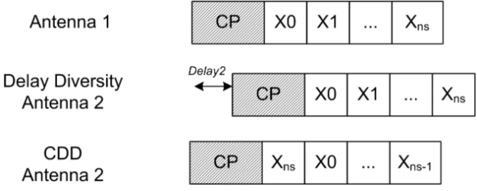
One of the first methods proposed to use spatial diversity was delay diversity [7]. This method transmits without delayed over the first antenna, while over the
Fig. 2.1: Delay diversity and Cyclic delay diversity OFDM frame
second or each additional antenna the signal is transmitted with an specific delay. However, the main disadvantage of this scheme is that delay diversity will cause inter-symbol interference, if the delay is too large. Therefore, in OFDM, the maximum delay is limited by the length of the guard interval and the memory of the channel.
To overcome this problem, CDD was initially proposed in [8], [9] and [10]. Instead of delaying the signal in second or each other antenna, the signal is cyclically shifted avoiding inter-symbol interference and any cyclic shift value can be chosen. Great advantages of CDD are receiver does not need additional complexity and can be implemented in current standards, and CDD can scale with the number of antennas without any rate loss, as it is different for other space-time codes. For example, CDD can be used with 3 transmission antennas and keep the rate of 1, instead, other orthogonal space-time codes are not easily adapted for 3 antennas and also incurs in loss of the rate.
In Fig. 2.1 we illustrate the difference between delay diversity and CDD. The transmitted signal from antenna 1 is not delayed while the signal on antenna 2 is delayed one position for delay diversity method and cyclically shifted one position for CDD. In CDD, the cyclic prefix is added after the cyclically shifted operation is done, instead in delay diversity, the cyclic prefix is added before the delayed operation.
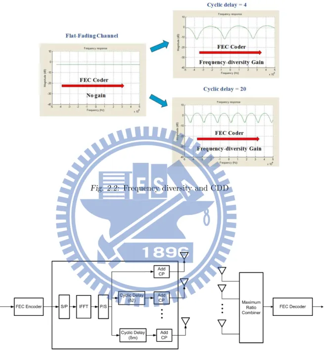
When we shift the OFDM signal cyclically, they are added at the receiver linearly inserting virtual echoes on the channel response or similar creating multi-paths at the receiver, thus higher frequency diversity can be achieved when exploited by any coded OFDM system. Fig. 2.2 represents how the channel is affected with CDD. In a flat fading channel, the frequency response of the channel is constant through all the subcarriers of the OFDM symbol. If we use a FEC coder across the subcarriers in the flat fading channel, the diversity gain is only 1, in other words, the FEC coder fails completely because when all subcarriers in the OFDM are in deep fade it becomes a burst error, it is well known that FEC coders cannot correct errors in burst error conditions. When applying a CDD with delay values of 4 or 20, the effective channel response seen at the receiver is not constant anymore becoming a frequency-selective channel, if the delay value is larger, more frequency selectivity is introduced in the channel as we observe in Fig. 2.2. The resultant channel still has the same BER results before coding as a flat fading channel but CDD change the distribution of the errors around the subcarriers and burst errors are not generated anymore. This is when it comes the benefits of using a FEC coder across subcarriers, consecutive subcarriers are not in deep fade anymore and FEC coding is able to obtain diversity gain in these conditions.
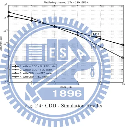
Fig. 2.3 shows a block diagram of CDD. At receiver a maximum ratio combiner is used to combine the received signals from different antennas. It is interesting to note that only one IFFT operation is required at the transmission side making it very simple and cost-effective. Fig. 2.4 shows simulation results for CDD in a MISO system with 2 TX antennas and 1 RX antenna. It clearly shows that from 4 cases, only one case where CDD and FEC coder is applied at the same time is able to gain diversity gain of around 2. Other cases failed completely in a flat fading channel of obtaining some diversity gain. This results is in accordance with the discussion exposed in previous paragraph.
Fig. 2.2: Frequency diversity and CDD
0 5 10 15 20 25 10−6 10−5 10−4 10−3 10−2 10−1 100 Eb/No, dB
Bit Error Rate
Flat Fading channel, 2 Tx − 1 Rx. BPSK.
1. Without CDD − No FEC coder. 2. Without CDD − FEC coder. 3. With CDD − No FEC coder. 4. With CDD − FEC coder.
4 1,2,3
CDD still needs more attention from the research community because it has great potential for future wireless technologies, for instance, it is suggested that when CDD is implemented in the downlink channel it can help improve the performance in the uplink [11]. This is due to CDD which creates virtual antennas or beamforming but the subscriber substation (SS) does not need to know that CDD has been applied, SS can use an antenna selection criterion shown in the paper that maximizes the uplink signal-to-noise ratio perceived at the base station.
2.2
Double Space Time Transmit Diversity
(DSTTD)
So far, most of the space-time codes try to improve the diversity gain of a system without trying to increase the capacity of it. With the emerging of new hungry data services over the wireless channel, it is imperative to try to find new schemes that can give better use of the spectrum. DSTTD surges as a competent option to improve the capacity of the system. Most relevant works about DSTTD are in [12], [13] and [14]. DSTTD achieves increased of the capacity, by combining space-time code and spatial multiplexing. It divides the total number of transmit antennas in groups of 2 and each group applies a space-time code, mostly Alamouti space-time code, in parallel. At the receiver side, it is required to detect each group using a group receiver, after this, each group detected is processed as if it was a pure space-time code. The group receiver is able to suppress the inter-block interference and keep the structure of each space-time block. It is called double space time transmit diversity because it is mostly associated when using 4 antennas at the transmission side, therefore only two space-time code groups are used. Fig. 2.5 illustrates a block diagram of DSTTD for an antenna configuration of 4Tx-4Rx. DSTTD is a rate 2 space-time code.
Fig. 2.5: Block diagram of DSTTD 0 5 10 15 10−6 10−5 10−4 10−3 10−2 10−1 Eb/No, dB
Bit Error Rate
MMSE−SIC GROUP
We evaluate the performance of DSTTD in a MIMO-OFDM system using a minimum-mean-square-error algorithm with successive interference cancellation (MMSE-SIC) group receiver. A MMSE-SIC group receiver filters the first group send from the transmission side, detects the first group and substracts its estimate from the received signal. The simulation results in Fig. 2.6 shows that the diversity gain obtained by the system is around 3. This results agree with similar results obtained in [12]. We use DSTTD extensively during this thesis as a comparison point for our results.
2.3
System Model
In this section, we introduce the system model that will be used through the rest of the thesis.
2.3.1
MIMO System Model
We considered a space-time coded single-user system with M transmit antennas and N receive antennas. The channel impulse response from transmit antenna m to receive
antenna n is given by the [1 × Ns] vector
hnm = [hnm(0), hnm(1), · · · , hnm(D), 0, · · · , 0], (2.1)
where D is the memory of the channel and Ns is the number of subcarriers of the
OFDM symbol, i.e., FFT size of the OFDM modulator.
It is easier to deal with the frequency domain representation of the MIMO channel. This is given by
Hnm = [Hnm(0), Hnm(1), · · · , Hnm(Ns− 1)], (2.2)
obtained from the FFT of the channel impulse response from transmit antenna m to receive antenna n of equation (2.1). Note than when D=0, the channel becomes a
Fig. 2.7: MIMO Channel
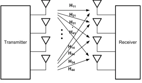
In Fig. 2.7, we can observe a graphical representation of the MIMO channel. It is common to represent the MIMO-OFDM channel in matrix form for each subcarrier. Grouping all channel coefficients from equation (2.2), we obtain the MIMO channel matrix for subcarrier kth
H(k) = H11(k) H12(k) · · · H1M(k) H21(k) H22(k) · · · H2M(k) ... ... . .. ... HN 1(k) HN 2(k) · · · HN M(k) , (2.3)
where k = 0, . . . , Ns − 1. We can observe from this representation that a
MIMO-OFDM system can be seen as Ns parallel single-carrier MIMO channels.
Final representation of the received signal for subcarrier kth is given by y(k) =
r 1
MH(k)s(k) + w(k), (2.4)
where y(k) is the received vector of size [N × 1], s(k) is the transmit vector of size [M × 1], w(k) is the additive white Gaussian noise (AWGN) vector [N × 1] with
Notice that the MIMO signal model in equation (2.4) is the frequency domain representation of the received signal, i.e., after removal of the cyclic prefix and FFT operation of the time domain received signal. For equation (2.4) to be valid the length of cyclic prefix for the OFDM symbol should be larger than the channel memory,
Analysis of Stacked Cyclic Delay
Diversity Schemes (SCDD)
In this chapter, we evaluate the performance of SCDD in a MIMO-OFDM system. The SCDD was first proposed in [15] where its diversity-multiplexing tradeoff was derived. To our knowledge, there are no other works in the literature evaluating the performance of SCDD, then, there is a big opportunity to explore more about this topic.
As we have discussed before, all transmit diversity schemes use all available degrees of freedom to obtain diversity. There is need for schemes that can explore diversity gain and multiplexing gain at the same time. DSTTD was one of the first schemes proposed to tackle this problem. DSTTD groups every two antennas and combined them as a STBC block. At the other end a linear receiver (ZF or MMSE) is used to separate both streams.
SCDD surges as a new possibility to affront this diversity-multiplexing tradeoff dilemma. Similar to DSTTD, SCDD groups several antennas and a CDD is applied on them, several CDD groups are stacked on top of each other and finally form the
stacked cyclic delay diversity scheme. Because transmit antennas are grouped, SCDD can be regarded as a kind of spatial-multiplexing system like V-BLAST. Therefore the same detection schemes used for V-BLAST or DSTTD can be adapted to SCDD. The two most common linear receivers used are zero-forcing (ZF) and minimum mean square error (MMSE). In this thesis we concentrate mostly on MMSE, but analysis of other receivers systems can be done in a straightforward manner.
3.1
Stacked Cyclic Delay Space-Time Code
For the stacked cyclic delay scheme we divide the total number of transmit antennas,
M, into G groups. Each group is equipped with nt transmit antennas, where M =
Gnt. Then, for each group a CDD is applied, having several CDD schemes stacked
on top of each other.
The SCDD scheme can be seen as a space-time code. A length-Ns space-time
code can be represented as an [M × Ns] matrix C,
C = s1(0) s1(1) · · · s1(Ns− 1) s2(0) s2(1) · · · s2(Ns− 1) ... ... . .. ... sM(0) sM(1) · · · sM(Ns− 1) , (3.1)
where sm(k) is the code symbol assigned to the mth antenna at subcarrier k.
To establish the relationship with equation (2.4), the matrix C is constructed as
C = [s(0), s(1), . . . , s(Ns− 1)], (3.2)
where s(k) is given by
In other words the columns of matrix C corresponds to the transmit vector in equation (2.4).
A FEC coder is used in CDD to achieve the frequency diversity gain. The
output of the FEC coder is composed by symbols [x0, x1, . . . , xL−1] where L is the
number of elements to be mapped to the space-time code. For an easier representa-tion, we split them in several vectors given by
xw = [xwL/G−L/G, xwL/G−L/G+1, . . . , xwL/G−1], (3.4)
where w = 1, . . . , G and xw indicates a vector for each CDD group w. It can be seen
that the number of output elements from the FEC coder is L = GNs.
As a final step, the mapping of vectors xw to matrix C according to system
parameters N, G, nt and Ns, is realized in the following way
C = x1(0) · · · x1(Ns− 1) ... . .. ... x1(Ns− δnt) · · · x1(Ns− δnt − 1) x2(0) · · · x2(Ns− 1) ... . .. ... xG(Ns− δM) · · · xG(Ns− δM − 1) . (3.5)
The cyclic delay value applied to each antenna is represented as δm, m = 1, . . . , M.
The purpose of matrix (3.5) is to have a generalized form to represent the stack cyclic diversity scheme. This representation can be helpful to analyze the performance from a space-time code point of view.
It is necessary to determine the rate of the space-time code, the rate will determine how many streams are sent at the same time. For SCDD is easily to observe that the rate is equal to G, i.e., the number of CDD groups in the scheme. The rate of the space-time code equals to the maximum spatial-multiplexing gain.
Another way to calculate the rate of the space-time code for SCDD is using L = GNs
and considering an OFDM symbol as Ns time slots, then, we have L code symbols to
transmit in Ns time slots,
RateSCDD = L Ns = GNs Ns = G. (3.6)
Let us examine how matrix C and transmit vector s(k) are formed with system
parameters M = 4, N = 4, Ns = 128, G = 2 and nt = 2. The output of the FEC
coder has L=256 symbols [x0, x1, . . . , x255] and the cyclic delays corresponding to
each antenna are δ1 = 0, δ2 = 1, δ3 = 0, δ4 = 1, then
x1 = [x0, x1, . . . , x127], (3.7)
x2 = [x128, x129, . . . , x255], (3.8)
and matrix C of size [4 × 256] is formed according to (3.5)
C = x1(0) x1(1) x1(2) · · · x1(127) x1(127) x1(0) x1(1) · · · x1(126) x2(0) x2(1) x2(2) · · · x2(127) x2(127) x2(0) x2(1) · · · x2(126) . (3.9)
To form the transmit vector we just need to get each column of matrix C and form the vector s(k) as (3.2) and (3.3), for example,
s(0) = [x1(0), x1(127), x2(0), x2(127)]T, (3.10)
is the first column of (3.9).
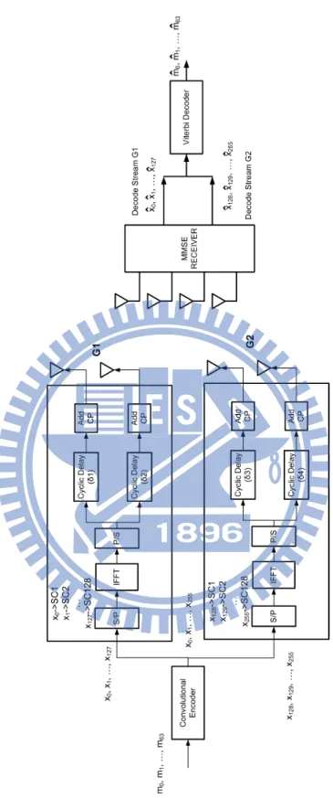
In Fig. 3.1, a block diagram of the whole SCDD scheme is shown. This is a 4x4 MIMO-OFDM system and m = 0, . . . , 63 is the input to the system, then a
one stream for each CDD group. Next, the mapping to subcarriers is realized where SCx is subcarrier x of the OFDM symbol. The IFFT operation is realized to each stream and a cyclic shift delay is applied to the time-domain signal according to values
δm. Note that only two IFFT operations are required in this case instead of 4, the
number of transmit antennas. A linear MMSE receiver is applied at the receiver to estimate the values of each stream, both streams are concatenated to form the input to the convolutional decoder that will finally estimate the initial input to the system m0, m1, . . . , m63.
3.2
Decoding SCDD - MMSE Receiver
Detection of SCDD can be realized in a similar fashion as V-BLAST or DSTTD, due that several antennas are grouped and the whole system can be considered as a spatial-multiplexing system. Zero forcing (ZF) or minimum mean square error (MMSE) receivers are most commonly used. We focus on MMSE in this thesis only. To proceed, we need to adjust the system model and use the concept of equiv-alent channel. Equivequiv-alent channel or also named effective channel, was considered first in [16] and [17]. With the equivalent channel representation we incorporate the
actual channel and the space-time code SCDD in one matrix ˆH, then the MMSE
receiver is applied to the equivalent channel.
For the new channel model we include the matrix for the cyclic delays. The representation is in the frequency-domain and is given by
y(k) = r
1
MH(k)D(k)u(k) + w(k), (3.11)
and H(k) is represented with the same structure as (2.3).
xw, u(k) = [x1(k), . . . , x1(k) | {z } nt , . . . , xG(k), . . . , xG(k) | {z } nt ]T. (3.12)
The cyclic delay is determined by the diagonal matrix,
D(k) = e−2πjkδ1/Ns 0 · · · 0 0 e−2πjkδ2/Ns 0 0 .. . . .. ... 0 · · · 0 e−2πjkδM/Ns . (3.13)
Combining matrix H(k) and D(k), we obtained
y(k) = r 1 M H11(k)e−2πjkδ1/Ns · · · H1M(k)e−2πjkδM/Ns H21(k)e−2πjkδ1/Ns · · · H2M(k)e−2πjkδM/Ns ... . .. ... HN 1(k)e−2πjkδ1/Ns · · · HN M(k)e−2πjkδM/Ns u(k) + w(k). (3.14)
To have a better picture of the derivation, we can evaluate the receiver at antenna 1, y1(k) =x1(k)[H1,1(k)e−2πjkδ1/Ns + . . . + H1,nt(k)e −2πjkδnt/Ns] + . . . + xG(k)[H(1,(G−1)(nt+1))(k)e −2πjkδ(G−1)(nt+1)/Ns + . . . + H 1,M(k)e−2πjkδM/Ns] + w1(k), (3.15) and combine the sums of all channels for each CDD group as
y1(k) =x1(k)[ nt X p=1 H1p(k)e−2πjkδp/Ns] + . . . + xG(k)[ M X p=(G−1)(nt+1) H1p(k)e−2πjkδp/Ns] + w1(k), (3.16)
and similarly we can form the received signal to each receiver antenna.
The matrix ˆH(k) can be formed using the equivalent channel seen at each
receive antenna. ˆH(k), a matrix of size [N × G], is given by
ˆ H(k) = Pnt p=1H1p(k)e−2πjkδp/Ns · · · PM p=(G−1)(nt+1)H1p(k)e −2πjkδp/Ns Pnt p=1H2p(k)e−2πjkδp/Ns · · · PMp=(G−1)(nt+1)H2p(k)e−2πjkδp/Ns ... . .. ... Pnt p=1HN p(k)e−2πjkδp/Ns · · · PMp=(G−1)(nt+1)HN p(k)e−2πjkδp/Ns .(3.17)
Each column of matrix ˆH(k) corresponds to the equivalent channel produced by each
CDD group.
At last, the new channel model is obtained
y(k) = r 1 MH(k)ˆ x1(k) x2(k) .. . xG(k) + w(k), (3.18)
where x1(k), . . . , xG(k) are the symbols transmitted for each stream. This new
chan-nel model allows us to decode each stream using a linear MMSE receiver. The MMSE filter is
WM M SE(k) = ( ˆH(k)HH(k) + σˆ n2IN)−1H(k)ˆ H, (3.19)
and applied to received signal ˆ x1(k) ˆ x2(k) ... ˆ xG(k) = WM M SE(k)y(k), (3.20)
3.3
Diversity-Multiplexing Tradeoff of SCDD
Analysis of diversity-multiplexing tradeoff of SCDD scheme was realized in [15] and it is given by the formula
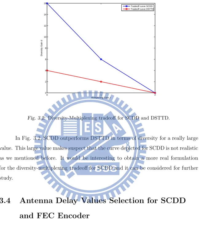
dSCDD(r) = nt(N − r)(G − r), (3.21)
where r = 0, . . . , G, G is the number of stacked CDDs, nt number of antennas used
for one group of CDD and N number of received antennas. According to equation (3.21), full diversity of the channel is achieved when r = 0, i.e., d(0) = MN. Also the maximum spatial multiplexing gain is exactly the number of stacked CDDs, i.e. d(G) = 0.
The analysis in [15] was realized with some constraints focusing on delay
op-timal codes, i.e., nt = Ns [18] and the interference between stacked CDD groups is
not consider. This scenario is too idealistic giving a result not achievable in a real-case scenario. From (3.21), it is possible to obtain the full diversity of the channel using SCDD considering that there is no interference between the groups. This is not possible using ZF or MMSE linear receivers and some interference will always be present after decoding each of the streams. The maximum spatial multiplexing gain achievable with SCDD is G and it does correspond to the value obtained in [15]. In other words, It is not possible to achieve the maximum diversity gain in a real scenario that formula (3.21) claims.
The results of [15] can be compared with the performance of DSTTD for the same number of antennas. Let us consider a SCDD with parameters M = N =
4, G = 2 and nt= 2, which is a very similar structure to DSTTD but instead of using
an Alamouti space-time code, a CDD is used between two antennas. Now, we can compare their diversity-multiplexing tradeoff curves depicted in Fig. 3.2, where the tradeoff for SCDD is obtained from equation (3.21).
0 1 2 0 2 4 6 8 10 12 14 16 Multiplexing Gain, r Diversity Gain d Tradeoff curve SCDD Tradeoff curve DSTTD
Fig. 3.2: Diversity-Multiplexing tradeoff for SCDD and DSTTD.
In Fig. 3.2, SCDD outperforms DSTTD in terms of diversity for a really large value. This large value makes suspect that the curve depicted for SCDD is not realistic as we mentioned before. It would be interesting to obtain a more real formulation for the diversity-multiplexing tradeoff for SCDD and it can be considered for further study.
3.4
Antenna Delay Values Selection for SCDD
and FEC Encoder
The selection of the delay values for each antenna of SCDD are a critical factor for its performance and a wrong selection would make the scheme to fail completely. Other works have already studied the delay values for CDD, [8], [19] and [20]. There are no
studies for the delay selection in SCDD, even though, it is possible to assume that the choices used for CDD can be also used for SCDD, we realize an analysis for SCDD in this section.
The FEC encoder is required to gain the frequency diversity added by SCDD, through this thesis we use a convolutional encoder as the FEC encoder. Convolutional encoders are very effective for overcoming fading channels ( [21], [22]). In [21] it is suggested that for block fading channels is required to use interleaving and the depth of the interleaving should be higher than the coherence time of the channel, then, consecutive bits from the output of the convolutional encoder experiment independent fading channels. Therefore, for SCDD, the best arrangement possible is to find the set of cyclic delay values that generates uncorrelated fading channels between adjacent subcarriers. It is required between adjacent subcarriers because the output stream of the convolutional encoder is mapped directly to consecutive subcarriers like is shown in Fig. 3.1.
For easier illustration, we select as system parameters M = 4, N = 4, Ns =
128, G = 2 and nt = 2 for SCDD. We can calculate the received signal in antenna 1
using equation (3.15) as,
y1(k) =x1(k)[H1,1(k)e−2πjkδ1/Ns+ H1,2(k)e−2πjkδ2/Ns]+
x2(k)[H1,3(k)e−2πjkδ3/Ns+ H1,4(k)e−2πjkδ4/Ns] + w1(k), (3.22)
and can be reduced using matrix ˆH(k) as,
y1(k) = x1(k) ˆH11(k) + x1(k) ˆH12(k) + w1(k). (3.23)
The elements x1(k) and x1(k + 1) are consecutive and mapped to adjacent
subcarriers, the same for x2(k) and x2(k + 1). We want their effective channels
ˆ
safe to assume that we can treat each CDD group as independent and is enough to analyze only one CDD group. To generate uncorrelated fading channels we select
δ1 = 0 and δ2 = Nnts, then
ˆ
H11(k) = H1,1(k) + H1,2(k), for even subcarriers and
ˆ
H11(k) = H1,1(k) − H1,2(k), for odd subcarriers. (3.24)
As we indicated before the MIMO channel H is spatially uncorrelated and power delay profiles from different transmit antennas are the same. Similar we can assume that the coherence bandwidth of the channel is larger than two subcarriers. These assumptions can be expressed like
E{H1,1(k)H1,2(k)∗} = 0,
E{|H1,1(k)|2} = E{|H1,2(k)|2} and
H1,1(k) ≈ H1,2(k + 1). (3.25)
Now we can calculate the correlation between adjacent subcarriers for the
effective channel, representing ˆH11(2k) for even subcarriers and ˆH11(2k) for odd
p2k,2k+1 = E{ ˆH11(2k) ˆH11(2k + 1)∗} = E{(H1,1(2k) + H1,2(2k))(H1,1(2k + 1) + H1,2(2k + 1))∗} = E{|H1,1(k)|2} + E{H1,1(2k)H1,2(2k + 1)∗} − E{H1,2(2k)H1,1(2k + 1)∗} − E{|H1,2(k)|2} = E{|H1,1(k)|2} − E{|H1,1(k)|2}+ E{H1,1(2k)H1,2(2k)∗} − E{H1,2(2k)H1,1(2k)∗} = 0. (3.26)
Similar procedure can be realized for the other CDD group selecting δ3 = 0
and δ4 = Nnst and it is concluded that in SCDD the delay selection can be realized
independently for each CDD group. Therefore, the selection would depend of the
number of antennas for each group (nt). Finally, the equation for the delay selection
is δp = 0, if (p − 1) mod nt = 0 NS nt + δp−1, otherwise (3.27)
where p = 1, . . . , M. With this set of cyclic delay values, it is guaranteed that adjacent subcarriers are uncorrelated or have low correlation and when consecutive bits of the convolutional encoder are assigned to adjacent subcarriers, the maximum frequency diversity can be obtained.
Other important factor to select is the minimum free distance of the convolu-tional encoder. Diversity gains obtained with the convoluconvolu-tional encoder are related
to the free distance of the code [23], [24]. From [23] it is concluded that to achieve the full diversity of the channel the minimum free distance of the code should be
df ree ≥ Maximum diversity of the channel. (3.28)
To our advantage, equation (3.28) assumes that fading channels across the symbols should be independent, condition that it is guaranteed in SCDD when calculating the cyclic delay values through equation (3.27).
In a MIMO channel the maximum diversity available is MaxDivChannel = DNM, where D is the channel memory, M number of transmit antennas and N number of receive antennas. For SCDD, each CDD group uses only a subset of the
transmit antennas (nt), then maximum diversity available is reduced. As each CDD
group is independent we can define that the maximum diversity possible for each
CDD group is MaxDivCDDGroup = DNnt. Therefore, the minimum free distance
of the convolutional encoder for SCDD is given by
df reeSCDD ≥ DNnt. (3.29)
A more formal analysis for the minimum free distance can be realized using matrix C and its bounds on pairwise error probability and it is considered for further study.
3.5
Numerical Results
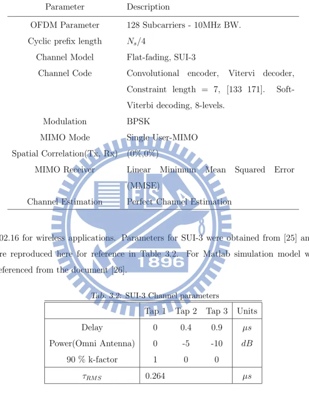
In this section, we show the numerical results for SCDD. Performance was evaluated through simulations in Matlab. In Table 3.1, the simulation parameters for SCDD are shown. We evaluate two cases of antenna configuration [4Tx,2Rx] and [4Tx,4Rx].
For SCDD, we use G = 2 and nt = 2, the rate of this space-time code is 2.
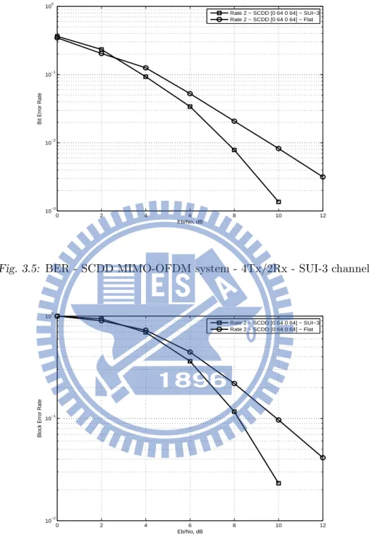
For the channel model, we evaluate in flat-fading channel and frequency-selective channel, SUI-3. SUI-3 is one of the channel models proposed in Wimax
Tab. 3.1: Simulation parameters for SCDD
Parameter Description
OFDM Parameter 128 Subcarriers - 10MHz BW.
Cyclic prefix length Ns/4
Channel Model Flat-fading, SUI-3
Channel Code Convolutional encoder, Vitervi decoder,
Constraint length = 7, [133 171].
Soft-Viterbi decoding, 8-levels.
Modulation BPSK
MIMO Mode Single User-MIMO
Spatial Correlation(Tx, Rx) (0%,0%)
MIMO Receiver Linear Minimum Mean Squared Error
(MMSE)
Channel Estimation Perfect Channel Estimation
802.16 for wireless applications. Parameters for SUI-3 were obtained from [25] and are reproduced here for reference in Table 3.2. For Matlab simulation model we referenced from the document [26].
Tab. 3.2: SUI-3 Channel parameters
Tap 1 Tap 2 Tap 3 Units
Delay 0 0.4 0.9 µs
Power(Omni Antenna) 0 -5 -10 dB
90 % k-factor 1 0 0
3.5.1
Results for 4Tx-2Rx
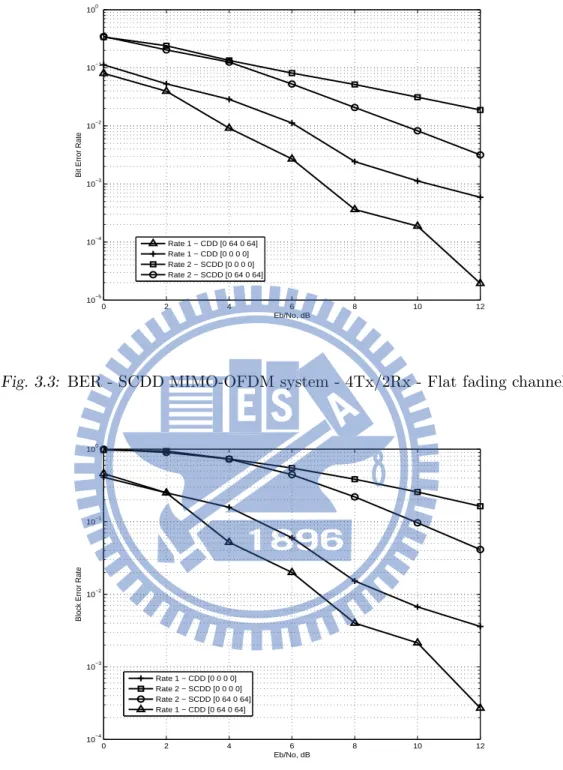
Fig. 3.3 and Fig. 3.4 shows the performance of SCDD in a flat fading channel. For the label of the legends, we indicate the cyclic delay of each transmission antenna
as SCDD [σ1σ2σ3σ4]. For example, SCDD [0 64 0 64], means that antenna 1 has 0
symbols of cyclic shift delay, antenna 2 has 64 symbols of cyclic shift delay, antenna 3 has 0 symbols of cyclic shift delay and antenna 4 has 64 symbols of cyclic shift delay. We also compare with a rate 1 pure CDD system. Pure CDD can be considered a
subset of SCDD with parameters G = 2 and nt = 4.
We show in Fig. 3.3 the improvement in diversity when CDD is applied to the system. We observe that the diversity gain for Rate 2-SCDD[0 0 0 0] is only 1, meanwhile, the diversity gain for Rate 2-SCDD[0 64 0 64] is 2. This proves that the convolutional encoder can pick up the frequency diversity added by the SCDD system. It is obvious that the pure CDD system has higher diversity gain because all available degrees of freedom are used for that purpose. In Fig. 3.4, we evaluate the performance in terms of block error rate. We consider a block as the same as one OFDM symbol. The results are similar to the bit error curve, where the Rate 2-SCDD[0 64 0 64] is able to pick up the diversity gain.
Fig. 3.5 and Fig. 3.6 show the performance of SCDD in a SUI-3 channel, which is frequency-selective. We observe in Fig. 3.5 that the system has higher diversity than in a flat-fading channel. The diversity gain is approximately 3. The reason is that the channel is already frequency-selective, then the convolutional encoder can obtain higher frequency-diversity than in a flat-fading channel. Similar for BLER curve, a higher diversity is obtained in a frequency-selective channel.
3.5.2
Results for 4Tx-4Rx
Fig. 3.7 and Fig. 3.8 show the performance of SCDD in a flat fading channel. The rate of SCDD keeps the same value of 2. Therefore, SCDD parameters are G = 2
and nt = 2. In Fig. 3.7, diversity gain obtained by SCDD [0 0 0 0], without CDD,
is around 2, meanwhile, the diversity gain of SCDD [0 64 0 64] is around 4, double the value when there is no CDD in the system. We also compare with DSTTD when using a MMSE-SIC receiver. Diversity gain of DSTTD with MMSE-SIC is only 3. SCDD has better performance than DSTTD using similar receiver architecture. In Fig. 3.8, results obtained for block error rate have similar conclusion where SCDD[0 64 0 64] is able to exploit the frequency-diversity added by the scheme.
Fig. 3.9 and Fig. 3.10 show the performance of SCDD in the frequency-selective channel SUI-3. Because the channel is already frequency-frequency-selective, the con-volutional encoder is able to exploit more frequency-diversity and obtain higher di-versity gains. In Fig. 3.9, SCDD[0 0 0 0] has a didi-versity of around 4, meanwhile, the diversity gain obtained when adding CDD (SCDD[0 64 0 64]) is slightly higher than 5. Interesting to compare with DSTTD, it is that DSTTD in a MIMO-OFDM system cannot obtain any higher performance from a frequency-selective channel. As the results show, DSTTD has the same performance in Fig. 3.9 and Fig. 3.7. The
reason is because a MIMO-OFDM system converts the system in a set of Ns parallel
single carrier MIMO channels, which is one of the advantages for OFDM because it allows simple equalizers at the receiver-end but loses the frequency-diversity present in the channel. Instead, SCDD already includes a convolutional encoder that takes advantage of the characteristics of the SUI-3 channel.
0 2 4 6 8 10 12 10−5 10−4 10−3 10−2 10−1 100 Eb/No, dB
Bit Error Rate
Rate 1 − CDD [0 64 0 64] Rate 1 − CDD [0 0 0 0] Rate 2 − SCDD [0 0 0 0] Rate 2 − SCDD [0 64 0 64]
Fig. 3.3: BER - SCDD MIMO-OFDM system - 4Tx/2Rx - Flat fading channel
0 2 4 6 8 10 12 10−4 10−3 10−2 10−1 100 Eb/No, dB
Block Error Rate
Rate 1 − CDD [0 0 0 0] Rate 2 − SCDD [0 0 0 0] Rate 2 − SCDD [0 64 0 64] Rate 1 − CDD [0 64 0 64]
0 2 4 6 8 10 12 10−3 10−2 10−1 100 Eb/No, dB
Bit Error Rate
Rate 2 − SCDD [0 64 0 64] − SUI−3 Rate 2 − SCDD [0 64 0 64] − Flat
Fig. 3.5: BER - SCDD MIMO-OFDM system - 4Tx/2Rx - SUI-3 channel
0 2 4 6 8 10 12
10−2 10−1 100
Eb/No, dB
Block Error Rate
Rate 2 − SCDD [0 64 0 64] − SUI−3 Rate 2 − SCDD [0 64 0 64] − Flat
0 1 2 3 4 5 6 7 8 9 10 10−5 10−4 10−3 10−2 10−1 100 Eb/No, dB
Bit Error Rate
SCDD [0 0 0 0] SCDD [0 64 0 64] DSTTD 4x4
Fig. 3.7: BER - SCDD MIMO-OFDM system - 4Tx/4Rx - Flat fading channel
0 1 2 3 4 5 6 7 8 9 10 10−4 10−3 10−2 10−1 100 Eb/No, dB
Block Error Rate
SCDD [0 64 0 64] SCDD [0 0 0 0]
0 1 2 3 4 5 6 7 8 9 10 10−5 10−4 10−3 10−2 10−1 100 Eb/No, dB
Bit Error Rate
SCDD [0 64 0 64] SCDD [0 0 0 0] DSTTD 4X4
Fig. 3.9: BER - SCDD MIMO-OFDM system - 4Tx/4Rx - SUI-3 channel
0 1 2 3 4 5 6 7 8 9 10 10−3 10−2 10−1 100 Eb/No, dB
Block Error Rate
SCDD [0 64 0 64] SCDD [0 0 0 0]
3.5.3
Summary
In Table 3.3, we present a summary of the results for SCDD. It is clear that SCDD pro-vides a better performance compared with DSTTD in the same antenna configuration of [4Tx - 4Rx]. The difference is higher for the SUI-3 channel because DSTTD can-not obtain frequency diversity gains from a frequency-selective channel. In a reduced configuration of receive antennas [4Tx - 2Rx], SCDD still can provide diversity gains attractive enough to consider it as a potential scheme for future wireless standards.
Tab. 3.3: Diversity Gains for Rate 2-SCDD and Rate 2-DSTTD
Flat-fading Channel SUI-3
SCDD(4Tx - 2Rx) 2 3
SCDD(4Tx - 4Rx) 4 5
Stacked Hybrid Cyclic Delay
Diversity Scheme (SHCDD)
In this chapter, we present a new scheme named stacked hybrid cyclic delay diversity (SHCDD) in a MIMO-OFDM System. This new scheme surges as an option to further increase the multiplexing gains obtained using schemes like SCDD and DSTTD.
In previous chapter we analyzed and discussed the performance of SCDD, we showed that the rate of this space-time code is equal to G, the number of CDD stacked groups. The rate will depend of the arrangement of antennas and how they are stacked together, then G will increase in integer values of 1, 2, ..., etc. In SCDD, the rate is only possible to increase in integer values, but there should be a scheme that still can explore intermediate rate values, e.g., 1.25, 1.40, etc. Most surprisingly is that SCDD still leaves a big gap between the maximum rate achievable by the scheme and maximum multiplexing gain possible in the MIMO channel. For example, in a system with 4 transmit antennas and 4 receiver antennas, the maximum multiplexing gain offered by the channel is 4, but the rate of the space-time code obtained using SCDD or DSTTD is only 2. There are still more rate values that are possible to explore,
e.g., 2.5 and 3.0.
4.1
Overview of SHCDD
As we mentioned before, SHCDD surges as an option to achieve higher space-time codes rates that schemes like SCDD cannot obtain. In SCDD, the same OFDM sym-bol is cyclic shifted in different antennas and then transmitted, all OFDM subcarriers are involved in the CDD process. For SHCDD to obtain higher rates, it considers that not all subcarriers are required to be involved in the CDD process and these subcarriers can be used for pure spatial multiplexing gain.
To have a better understanding of SHCDD is easier to represent it using an
example. Consider a system with M = 4, N = 4 and Ns = 6. In SCDD, with G = 2,
the matrix C will be formed from the vector xw as
C = x1(0) x1(1) x1(2) x1(3) x1(4) x1(5) x1(5) x1(0) x1(1) x1(2) x1(3) x1(4) x2(0) x2(1) x2(2) x2(3) x2(4) x2(5) x2(5) x2(0) x2(1) x2(2) x2(3) x2(4) . (4.1)
where the cyclic delays are δ1 = 0, δ2 = 1, δ3 = 0, δ4 = 1. The rate of this space time
code can be defined as how many symbols are transmitted during certain time slots.
In this case, 12 symbols (x1(0), . . . , x1(5), x2(0), . . . , x2(5)) are transmitted during
Ns = 6 time slots generating a rate 2 space-time code.
SHCDD takes advantage that some of those symbols are not required to be repeated and can be used to obtain higher multiplexing gain. If we want to form a
higher rate code, we can transform matrix C as this example C = x1(0) x1(1) x1(2) x1(3) x1(4) x1(5) x1(6) x1(0) x1(1) x1(2) x1(3) x1(7) x2(0) x2(1) x2(2) x2(3) x2(4) x2(5) x2(6) x2(0) x2(1) x2(2) x2(3) x2(7) . (4.2)
We have introduced more symbols in the matrix, then 16 symbols (x1(0), . . . , x2(7))
are transmitted during Ns= 6 time slots. The rate of this new code is
RateSHCDD =
16
6 =
8
3 = 2.666, (4.3)
which is higher than the rate 2 code obtained with SCDD in (4.2). As we observe,
symbols (x1(4), x1(5), x2(4), x2(5), x1(6), x1(7), x2(6), x2(7)) are not repeated and not
used for CDD, then it is expected that the diversity performance of this new code is lower than the one obtained in SCDD. That is clear as there is always a tradeoff, increasing multiplexing gain involves reducing diversity gain of the system. In the same way, it is possible to add more symbols and obtain higher rate codes and different configurations. As a great advantage of SHCDD, the rate of the space-time code is very flexible to adjust.
SHCDD also allows to adjust its scheme to a more flexible number of transmit antennas. The minimum number of transmit antennas required for SCDD or DSTTD is 4, meanwhile, SHCDD can start from 2, 3, 4, ..., etc. transmit antennas. Let us
consider the case of M = 2, N = 2 and Ns = 6. This antenna configuration cannot
be used for SCDD or DSTTD but we can use it for SHCDD. As an example, a CDD scheme using two transmit antennas is given by
C = x1(0) x1(1) x1(2) x1(3) x1(4) x1(5) x1(5) x1(0) x1(1) x1(2) x1(3) x1(4) , (4.4)
where the rate of this space-time code is 1. Similar to previous case, we can increase the number of transmitted symbols as
C = x1(0) x1(1) x1(2) x1(3) x1(4) x1(5) x1(6) x1(0) x1(1) x1(2) x1(3) x1(7) , (4.5)
increasing the rate of the space-time code to RateSHCDD =
8
6 =
4
3 = 1.333, (4.6)
because we transmit 8 symbols (x1(0), . . . , x1(7)) in Ns = 6 time slots. SHCDD
proved to be a very flexible scheme to adjust the multiplexing gain of the MIMO-OFDM system.
4.2
Construction of SHCDD
In this section, we explain a more general representation of SHCDD and its con-struction. To make easier the construction of SHCDD, we only deal with one group (G = 1) and stacked them according to how many groups are required in the system. This group alone is called Hybrid CDD (HCDD). HCDD is similar to CDD except for the difference that some subcarriers are not used for CDD.
We define the concepts periodHCDD, SymbolsHCDD, clustersHCDD and
sub-carriersCDD, to help for the description of HCDD. The term periodHCDD refers to
how many subcarriers in an OFDM symbol form one cluster, SymbolsHCDD refers to how many symbols are transmitted in one cluster or similar in one periodHCDD and
clustersHCDD refers to how many clusters an OFDM symbol contains. A cluster for
a 2 transmission antenna system is formed as
Clusterq = x1(0) x1(1) · · · x1(p − 2) x1(p − 1) x1(0) x1(1) · · · x1(s − p − 1) x1(p) · · · x1(s − 1) x1(s) ,(4.7)
where p = periodHCDD, s = SymbolsHCDD and q = 1, . . . , clustersHCDD. In other words, a cluster is formed with p subcarriers and the last SymbolsHCDD
-periodHCDD subcarriers of antenna 2 are packed with extra symbols. The term subcarriersCDD refers to the number of subcarriers in a cluster that are repeated,
or in other way, the number of subcarriers where the CDD will be applied, and subcarriersCDD = 2 × periodHCDD − SymbolsHCDD.
Next, we concatenate several clusters and applied CDD to form the final HCDD group. The number of clusters is defined by
clustersHCDD = Ns
periodHCDD, (4.8)
where it is expected that clustersHCDD is a real number for easy construction of
SHCDD. Then, we group all the clusters in one matrix of size [2 × Ns],
GN oCDD= [Cluster1, Cluster2, . . . , ClusterclustersHCDD]. (4.9)
Notice that matrix GN oCDD has not included the cyclic shift in its vector for antenna
2. We named GCDD, the matrix that already includes the effect of cyclic shift in
antenna 2 (δ2). GCDD is finally consider one HCDD group.
The rate of the space-time code SHCDD is determined by
RateSHCDD = SymbolsHCDD
periodHCDD × G. (4.10)
These two parameters are widely configurable allowing to select the rate of the system more flexible. If SymbolsHCDD = periodHCDD, corresponds to SCDD.
At last, we construct the final system model for SCDD. The number of HCDD groups is determined by the system parameter G. The received signal is modeled as,
y(k) = r
1
MH(k)s(k) + w(k), (4.11)
where y(k) is the received vector of size [N × 1], s(k) is the transmit vector of size [M × 1], w(k) is the additive white Gaussian noise (AWGN) vector [N × 1] with
W ∼ CN (O, NoI) and H(k) is the MIMO channel model [N × M] for subcarrier kth.
The values s(k) are obtained from the matrix C given by
C = s1(0) s1(1) · · · s1(Ns− 1) s2(0) s2(1) · · · s2(Ns− 1) ... ... . .. ... sM(0) sM(1) · · · sM(Ns− 1) . (4.12)
Then, matrix C is formed from the stacked of G HCDD groups as
C = GCDD(1) GCDD(2) ... GCDD(G) . (4.13)
4.3
Decoding SHCDD - MMSE Receiver
Detection of SHCDD can be realized similar to SCDD, using a MMSE filter to decode different streams from different HCDD groups. But SHCDD requires two MMSE receivers, one to decode the subcarriers where CDD is applied and other MMSE receiver to decode the subcarriers where CDD is not applied.
We define two MMSE receivers: The first MMSE receiver uses the same same model exposed in chapter 3 using the concept of equivalent channel. The MMSE filter is
where ˆ H(k) = Pnt p=1H1p(k)e−2πjkδp/Ns · · · PMp=(G−1)(nt+1)H1p(k)e −2πjkδp/Ns Pnt p=1H2p(k)e−2πjkδp/Ns · · · PM p=(G−1)(nt+1)H2p(k)e −2πjkδp/Ns ... . .. ... Pnt p=1HN p(k)e−2πjkδp/Ns · · · PM p=(G−1)(nt+1)HN p(k)e −2πjkδp/Ns .(4.15)
The second MMSE filter is applied directly to the MIMO channel to decode each stream of each transmit antenna,
WM M SE2(k) = (H(k)HH(k) + σ2nIN)−1H(k)H, (4.16)
where H is given by the MIMO channel from (2.3).
We define when to apply WM M SE1 or WM M SE2 in the following way. In
previous section, the term subcarriersCDD was defined as subcarriersCDD = 2 × periodHCDD − SymbolsHCDD indicating the number of subcarriers used for CDD in a cluster, we named these subcarriers as CDDsubcarriers. The others subcarriers are used for pure spatial multiplexing, we named these others as NonCDDsubcarriers.
The filter WM M SE1 is used for the first group of subcarriers that CDD is applied in
a cluster and WM M SE2 is used for the other subcarriers,
ˆ x1(k) ˆ x2(k) .. . ˆ xG(k) = WM M SE1(k)y(k), (4.17)
where k is the set of subcarriersCDD and ˆ x1(k) ˆ x2(k) ... ˆ xN(k) = WM M SE2(k)y(k), (4.18)
where k is the set of NonCDDsubcarriers. The two resultant vectors are of different size, therefore, it is required after the MMSE receiver a SHCDD detector that is in charge of arranging the order of the symbols to send to the Viterbi decoder.
In Fig. 4.1, a block diagram of a 4×4 MIMO-OFDM system using the SHCDD scheme is shown. SHCDD generator is in charge to create matrix C from the output of the convolutional encoder. SHCDD detector is in charge of determining what
subcar-riers are filtered with WM M SE1 or WM M SE2 and SHCDD combiner will concatenate
and group all symbols to send to the convolutional decoder.
4.4
Performance Analysis of SHCDD
To understand the performance of SHCDD it is necessary to as an unequal error prob-ability code (UEP). An UEP code is when not all bits transmitted over the channel have the same bit error probability performance with some bits having higher decoded error probability and other bits with less decoded error probability. UEP with con-volutional codes have been studied in [27]. Similar, puncturing concon-volutional codes are considered a form of UEP codes. Punturing a code corresponds to eliminate some of the output bits of the convolutional encoder, increasing the rate of the code. As a result the free distance is reduced and performance is affected as a trade off for obtaining a higher rate code. It is clear that the puncturing pattern, or decision of what bits are eliminated, is important for the performance of the code [28]. SHCDD can be considered in some way similar to a puncturing convolutional code and UEP codes. The difference is that SHCDD doesn’t eliminate some bits, but assigns some bits with more weight and others with less. From previous section, it was defined
CDDsubcarriers as the subcarriers that are used for CDD and NonCDDsubcarri-ers as the subcarriNonCDDsubcarri-ers used for pure spatial multiplexing, then, the bits assigned to CDDsubcarriers have lower probability of error and bits assigned to
carriers have higher probability of error. Then, a SHCDD can be considered as a
unequal error probability code.
In puncturing convolutional codes, the free distance of the code is reduced and performance is affected. This is obvious since some bits are not completely transmitted and they will be introduced randomly at the receiver end to be able to use the standard viterbi decoding. Similar as we increase the rate of the SHCDD code, we expect the performance to be lower due to the free distance of the code is reduced.
4.5
Numerical Results
In this section, we show the numerical results for SHCDD. Parameters for the simu-lation are presented in Tables 3.1 and 3.2. We evaluate two cases of antenna config-uration [2Tx,2Rx] and [4Tx,4Rx].
4.5.1
Results for 2Tx-2Rx
Fig. 4.2 shows results for different rates for SHCDD in a flat fading channel. We evaluate for rates 1.25, 1.33 and 1.40, and compare them with the Rate 1 - Pure CDD system and Rate 2 with full spatial multiplexing. To obtain the rates, parameters for SHCDD are as follow
• Rate 1.25: periodHCDD = 4 and SymbolsHCDD = 5. • Rate 1.33: periodHCDD = 3 and SymbolsHCDD = 4. • Rate 1.40: periodHCDD = 5 and SymbolsHCDD = 7.
In Fig. 4.2, we observe how the diversity gain is decreasing when the rate of the system is higher. This is clear because SHCDD at higher rates uses more time slots
0 5 10 15 10−6 10−5 10−4 10−3 10−2 10−1 100 Eb/No, dB
Bit Error Rate
Rate 2 − Spatial Multiplexing Rate 1 − CDD
Rate 1.25 − SHCDD [ 0 64 ] Rate 1.33 − SHCDD [ 0 64 ] Rate 1.40 − SHCDD [ 0 64 ]
Fig. 4.2: BER - SHCDD MIMO-OFDM system - 2Tx/2Rx - Flat fading channel
for spatial multiplexing and less of them for diversity gain. Also the convolutional encoder can only pick up the diversity gain from the time slots used for CDD. Diversity gain obtained for rate 1.25 SHCDD is around 2.5, meanwhile, the diversity gain for pure CDD system is slightly higher than 3. Diversity gain for rate 1.33 SHCDD is slightly lower than 2 and there is not diversity gain for rate 1.40 SHCDD system. The reason for rate 1.40 to not have any diversity gain can be understood from the parameters periodHCDD and SymbolsHCDD, where the output stream of the convolutional encoder, 3 consecutive symbols are transmitted using CDD and the next 4 consecutive symbols are transmitted with full spatial multiplexing, therefore the convolutional encoder is not able to gain any frequency diversity from the scheme.
4.5.2
Results for 4Tx-4Rx
In Fig. 4.3, we evaluate rates of 2, 2.5 and 3 for SHCDD. Parameters to obtain those rates are
• Rate 2.5: periodHCDD = 4 and SymbolsHCDD = 5 with G = 2. • Rate 3.0: periodHCDD = 4 and SymbolsHCDD = 6 with G = 2.
The scheme Rate 2.5 - SHCDD [0 64 0 64] provides a diversity gain of 4, meanwhile, the diversity gain from the same scheme but without CDD (SHCDD [0 0 0 0]) is 3. Therefore, the CDD introduced in the system can help to improve its performance. When comparing against DSTTD, the rate 2.5 SHCDD code has better
performance when Eb/No is higher than 8dB. The Rate 3 - SHCDD [0 64 0 64] code
has diversity gain slightly higher than 2 and it is clear that its performance is lower than rate 2 and 2.5 SHCDD schemes. Meanwhile, the rate 3 SHCDD code has better diversity gains than a rate 4 pure spatial multiplexing scheme where the diversity gain is only 1.
0 1 2 3 4 5 6 7 8 9 10 10−5 10−4 10−3 10−2 10−1 100 Eb/No, dB
Bit Error Rate
Rate 2 − SHCDD [0 0 0 0] Rate 4 − Spatial Multiplexing Rate 2.5 − SHCDD [0 64 0 64] Rate 3 − SHCDD [0 64 0 64] Rate 2 − SCDD [0 64 0 64] Rate 2 − DSTTD 4x4
Conclusions
In this dissertation, we concentrate mostly on resolving a dilemma of how to use the MIMO channel to achieve higher capacity without decreasing the reliability of our system. For resolving this problem, first we analyze the new scheme SCDD and give some performance results, interestingly to note is that SCDD has not been studied in detail in the research community, therefore, motivated by our results obtained here, we prove that SCDD has the potential to become a very promising technology. Second, we design a new scheme based on SCDD. We called this new scheme SHCDD, and explain the construction of its code and analyze some performance results.
The two major contributions from our dissertation are:
• Established the rules for parameters selection in SCDD. The evaluation of its results shown it can outperform current schemes proposed for MIMO channel. • Proposed a new scheme (SHCDD) that proved to be very flexible and more
ad-justable than SCDD. The space-time code rate can be adjusted to non-integer val-ues, condition that it is not possible for SCDD. Also as great advantage, SHCDD can be used in antenna configuration of 2Tx-2Rx, meanwhile, schemes like SCDD
and DSTTD are only designed for a minimum number of 4 transmission antennas.
5.1
Analysis of Stacked Cyclic Delay Diversity
Schemes (SCDD)
SCDD allows the MIMO channel to achieve a more optimal tradeoff between re-liability and transmission rate in the system. We showed that when using SCDD in a flat-fading channel the diversity gain is doubled compared to a system where no cyclic delays are applied in their transmission antennas. In a frequency-selective channel like SUI-3, the diversity gain is lower because the channel already provides some frequency-diversity to the system. We also compare in antenna configuration of 4Tx-4Rx, with current scheme DSTTD, and show that SCDD outperforms DSTTD in terms of diversity gain when using similar structure for the MMSE receiver. In-teresting to note is that in the SUI-3 channel, DSTTD cannot obtain any frequency-diversity gain from the system due to the condition that OFDM will treat DSTTD as several parallel single-carrier channels.
5.2
Stacked Hybrid Cyclic Delay Diversity
Scheme (SHCDD)
SHCDD proved to be a very flexible space-time code in terms of adjustable rate. Meanwhile, SCDD can only obtain integer rates, with SHCDD it is possible to reach non-integer values for its rate and therefore obtain a better optimal tradeoff between diversity and multiplexing gain according to system requirements. However its major drawback is that its performance is severely affected for higher rates due to the condition that when using a convolutional encoder, most of the symbols of the stream
will not experience any diversity and convolutional coding fails to pick up the diversity from the channel. In an antenna configuration of 2Tx-2Rx, this condition happens when the rate of the code is higher than 1.4. It seems that for the 4Tx-4Rx case this situation can be tolerated more, for instance, the rate 3 SHCDD system still can provide some diversity gain to the system. When comparing with DSTTD, we show that the proposed rate 2.5 SHCDD scheme has better performance, considering that the rate of the code is 25% higher.
5.3
Suggestions for future research
As we discussed before, we believe that currently not many research is being done or papers being published with topics around CDD. Only the 3GPP groups working for LTE and Wimax working groups are more active in this topic research. Therefore, there are countless options for future research related with CDD technologies and obtain better optimal tradeoffs for capacity and reliability. We numbered some of those suggestions that are more connected directly with our thesis:
• Obtain a more realistic analysis of the diversity-multiplexing tradeoff for stacked cyclic delay diversity schemes.
• Extend the research to multi-user MIMO scenarios, where we believe there are many interesting topics to analyze.
• Develop an analysis of SCDD and SHCDD with high performance-error correcting codes as Turbo codes to achieve higher capacity in the system.
• Design and evaluation of how to combine space time trellis codes with SCDD and SHCDD schemes.
• Analysis of SCDD and SHCDD in cooperative networks can be an interesting topic to research.
[1] M. Siavash and A. Alamouti, “A Simple Transmit Diversity Technique for Wire-less Communications,” IEEE Journal on select areas in communications, vol. 16(8), October 1998.
[2] A. Paulraj, R. Nabar, and D. Gore, Introduction to Space-Time Wireless
Com-munications. Cambridge Unversity Press, 2003.
[3] H. Jafarkhani, Space-time coding: theory and practice. Cambridge Unversity
Press, 2005.
[4] J. Tan and G. Stuber, “Multicarrier Delay Diversity Modulation for MIMO Sys-tems,” IEEE Transactions on Wireless Communications, vol. 3, September 2004. [5] L. Zheng and D. Tse, “Diversity and Multiplexing: A Fundamental Tradeoff in Multiple Antenna Channels,” IEEE Transactions on Information Theory, vol. 49(5), May 2005.
[6] 3GPP TS 36.211 V8.4.0, “3rd generation partnership project technical specifica-tion group radio access network evolved universal terrestrial radio access (e-utra) physical channels and modulation (release 8),” 2008-2009.
[7] N. Seshadri and J. H. Winters, “Two signaling schemes for improving the er-ror performance of frequency-division-duplex (FDD) transmission systems using transmitter antenna diversity,” International Journal of Wireless Information
Networks, vol. 1(1), March 1994.
[8] A. Huebner, M. Bossert, F. Schuehlein, and H. Haas, “On cyclic delay diversity in OFDM based transmission schemes,” International. OFDM Wksp, Hamburg,
Germany, 2002.
[9] Y. Zhang, J. Cosmas, K.-K. Loo, M. Bard, and R. D. Bari, “Analysis of cyclic de-lay diversity on DVB-H systems over spatially correlated channel,” IEEE Trans.
Broadcasting, vol. 53(1), March 2007.
[10] D. Gore, S. Sandhu, S. S, and A. Paulraj, “Delay diversity codes for frequency selective channels,” in In Proceedings of the IEEE International Conference on
[11] L. Jalloul, N. Czink, B. Hochwald1, and A. Paulraj, “Why Downlink Cyclic Delay Diversity Helps Uplink Transmit Diversity,” IEEE Vehicular Technology
Conference - Spring, 2009.
[12] L. Zhao and V. Dubey, “Detection schemes for space-time block code and spa-tial multiplexing combined system,” IEEE Communication Letters, vol. 9(1), January 2005.
[13] K. Kwak, J. Kim, B. Park, and D. Hong, “Performance analysis of DSTTD based on diversity-multiplexing trade-off,” IEEE Vehicular Technology Conference, vol. 61(2), 2005.
[14] G. Capponi, Y. Zheng, A. Gumaste, and C. Xiao, “Error Performance of Dou-ble Space Time Transmit Diversity System,” IEEE International Conference on
Communications, 2006.
[15] A. Sezgin, M. Charafeddine, S. Pereira, and A. Paulraj, “Diversity-multiplexing tradeoff of stacked cyclic delay diversity schemes,” in Conf. On Comm., Control,
and Computing, Monticello, Illinois, USA, September 26- 28 2007.
[16] B. Hassibi and B. Hochwald, “High-rate codes that are linear in space and time,”
IEEE Transactions on Information Theory, vol. 48(7), July 2002.
[17] S. Sandhu and A. Paulraj, “Space-time block codes: A capacity perspective,”
IEEE comm. Letters, vol. 4(12), December 2000.
[18] V. Tarokh, H. Jafarkhani, and A. Calderbank, “Space-time block codes from orthogonal designs,” IEEE Transactions on Information Theory, vol. 45(5), July 1999.
[19] G. Bauch and J. S. Malik, “Cyclic delay diversity with bit-interleaved coded mod-ulation in Orthogonal frequency division multiple access,” IEEE Transactions on
Wireless comunications, vol. 5(8), August 2006.
[20] G. Bauch and J. Shamim, “Parameter optimization, interleaving and multiple access in OFDM with cyclic delay diversity,” IEEE Transactions on Wireless
comunications, vol. 5(8), August 2006.
[21] E. Malkam and H. Leib, “Evaluating the Performance of Convolutional Codes Over Block Fading Channels,” IEEE Transactions on Information Theory, vol. 45(5), July 1999.
[22] G. Caire, G. Taricco, and E. Biglieri., “Bit-interleaved coded modulation,” IEEE
Transactions on Information Theory, vol. 44, May 1998.
[23] D. Tse and P. Viswanath, Fundamentals of wireless communication. Cambridge University Press, 2004.