基於雲端運算公有雲之資源利用率分析與預測框架

國

立

交

通

大

學

資訊科學與工程研究所

碩

士

論

文

基於雲端運算公有雲之資源利用率分析與

預測框架

A Flexible Analysis and Prediction Framework

on Resource Usage in Public Clouds

研 究 生： 林家瑜

指導教授： 曾煜棋 教授

王蒞君 教授

基於雲端運算公有雲之資源利用率分析與預測框架

A Flexible Analysis and Prediction Framework on Resource Usage in Public Clouds

研 究 生： 林家瑜 Student：Chia-Yu Lin

指導教授： 曾煜棋 Advisor：Yu-Chee Tseng

王蒞君 Li-Chun Wang

國 立 交 通 大 學

資訊科學與工程研究所 研 究 所

碩 士 論 文

A Thesis

Submitted to Department of Computer Science College of Computer Science

National Chiao Tung University in partial Fulfillment of the Requirements

for the Degree of Master

in

基於雲端運算公有雲之資源利用率分析與預測框架

學生: 林家瑜 指導教授: 曾煜棋 王蒞君 教授 國立交通大學資訊科學與工程學系(研究所)碩士班

摘 要

在雲端基礎設施服務(Infrasructure as A Service )裡，使用者可以向雲端服務的提供 者承租虛擬機器來執行它們的程式，但是虛擬機器有多種的規格，使用者對於自己的程 式應該花多少個虛擬機器來執行毫無概念。因此，我們提出了一個可以預估資源的服務 框架，此服務框架能夠告訴使用者對於即將執行的程式需要最少需要多少個虛擬機器執 行才能在特定的時間內完成，為了驗證此預估資源的服務框架可行性，我們還做了一些 範例的研究，由於 Frequent Pattern Growth (FP-growth)、K-means、Particle Swarm Optimization (PSO)的輸入資料皆相當大量，運算複雜，因此我們將此三種演算法修改成 平行化的執行方式，並運行在此框架底下進行資源預估，實驗結果顯示我們此框架可以 成功地針對某一個新來的工作預估出在特定時間內完成所需要的虛擬機器個數。另外， 從範例演算法中得知此框架不僅可運行輸入資料量小的工作，亦適用於輸入資料很大量 的工作，此框架相當彈性，此彈性化以及實用的框架讓使用者在租用虛擬機器時不會租 太多虛擬機器而浪費錢，也讓雲端服務的提供者能夠更方便地管理系統內的虛擬機器。 關鍵字: 資源預估框架、虛擬機器、平行化FP-growth、平行化K-means

A Flexible Analysis and Prediction Framework

on Resource Usage in Public Clouds

Student: Chia-Yu Lin Advisor: Prof. Yu-Chee Tseng

Prof. Li-Chun Wang Department of Computer Science, National Chiao Tung University

ABSTRACT

In cloud computing environments, users can rent virtual machines (VMs) from cloud providers to execute their programs or provide network services. While using this kind of cloud service, one of the biggest problems for the users is that how many VMs are needed to complete the jobs without spending too much money and time. In this paper, we propose a resource prediction framework (RPF) which can help users rent the minimum number of virtual machines and complete their jobs within a user specified time constraint. In order to verify the feasibility of RPF, we have done 3 case studies, parallel frequent pattern growth (FP-Growth), parallel K-means and Particle Swarm Optimization (PSO), on the proposed framework. FP-growth, K-means and PSO are data intensive algorithms. These algorithms may be executed repeatedly with different execution parameters to find the optimal results. When evaluating RPF by these algorithms in cloud environments, we have to modify them to parallel versions. The evaluation results indicate that RPF can successfully obtain the minimum number of VMs with acceptable errors. According to the results of case studies, the proposed RPF can be adopted by data intensive jobs, which is flexible and useful for users and cloud system providers.

Keywords: resource prediction framework, virtual machines, parallel FP-growth,

致謝

首先特別要感謝的是我的指導老師曾煜棋教授以及王蒞君教授。每兩週與老 師討論碩論內容，曾老師常常能在短時間內就點出我的一些盲點，即時修正，讓 我能順利完成碩士口試畢業；王老師則是時常反問我碩士論文的貢獻以及創新點， 讓我能在碩士論文的撰寫中更能強調作品的貢獻以及價值。另外，要感謝各位 HSCC 實驗室的學長姊們常能與我們討論給予一些經驗，讓我們在修課以及研 究上更加順利，尤其要感謝陳彥安學長的指導，學長在每週的討論總會給予適當 的意見及幫助，在論文的撰寫方面也給予許多重要的提點以及方向修正，口試完 後還幫我修改投稿的論文，非常謝謝學長。除了實驗室的學長姐外，還要感謝實 驗室的好夥伴、好同學在這兩年間各方面的幫忙，有你們的幫忙讓我的碩士生涯 更加充實與豐富。最後，要感謝我的家人在我就讀交大的路途上一路支持著我， 謝謝你們這兩年間的包容與體諒，讓我得以順利完成碩士學位。

Contents

Chinese Abstract i

Abstract ii

Acknowledgements (Chinese) iii

1 Introduction 1 2 Related Work 3 3 SYSTEM DESIGN 4 4 RPF Algorithms 6 4.1 Training Algorithm . . . 7 4.2 Prediction Algorithm . . . 7 5 Case Study 10 5.1 FP-growth . . . 10 5.1.1 Parallel FP-growth . . . 11 5.1.2 Parallel FP-growth on RPF . . . 13

5.1.3 Parallel FP-growth on RPF Experiment Setup . . . 14

5.1.4 Evaluation . . . 15

5.2 K-means . . . 15

5.3 PSO . . . 20

5.3.1 Parallel PSO on RPF . . . 21

5.3.2 Parallel PSO on RPF Experiment Setup . . . 22

5.3.3 Evaluation . . . 22

List of Figures

3.1 System architecture. . . 5

5.1 The execution scenario of FP-growth. . . 11

5.2 Constructing FP-trees. . . 11

5.3 Conditional tree and result of FP-growth. . . 12

5.4 MapReduce counting in Parallel FP-growth. . . 12

5.5 The execution process of parallel FP-growth. . . 13

5.6 The example of training algorithm by FP-growth. . . 13

5.7 The example of prediction algorithm 1 by FP-growth. . . 14

5.8 The example of prediction algorithm 2 by FP-growth. . . 14

5.9 The prediction curve of FP-growth by prediction algorithm 1. . . 15

5.10 The prediction curve of FP-growth by prediction algorithm 2. . . 16

5.11 RMSE of prediction algorithm. . . 17

5.12 The example of K-means. . . 18

5.13 The execution example of parallel K-means. . . 19

5.14 The example of training algorithm by K-means. . . 20

5.15 The example of prediction algorithm 1 by K-means. . . 20

5.16 The example of prediction algorithm 2 by K-means. . . 21

5.17 The prediction curve of K-means by prediction algorithm 1. . . 21

5.18 The prediction curve of K-means by prediction algorithm 2. . . 22

5.19 RMSE of prediction algorithm. . . 23

Chapter 1

Introduction

Cloud computing provides the users with a large number of computing and storage re-sources. By renting the resource from cloud provider, the users could avoid the hardware investment and maintenance cost. The services of cloud computing is generally classified into 3 service types, software as a service (SaaS), platform as a service (PaaS) and in-frastructure as a service (IaaS). Amazon Elastic Compute Cloud (Amazon EC2), which is an IaaS provider, provides many types of VMs with different EC2 computing units and memory sizes. The billing method is based on chosen VM capabilities and the rented time period. MapReduce is a parallel programming platform for users to develop parallel pro-grams in cloud environments. While users analyze the massive data in a cloud database, the parallel execution can reduce the execution time intensively. However, users usually do not know how many VMs they really need to execute a job. There is a trade-off be-tween the rented VM numbers and the execution time of a job. Therefore, we propose a resource prediction framework (RPF) which predicts the minimum number of VMs for a MapReduce job under a user specified time constraint.

The proposed RPF consists of training and prediction algorithms. In training algo-rithm, users execute their parallel jobs with different execution parameters and the system records the execution parameters, execution time and allocated VM numbers. After col-lecting enough information, the training algorithm analyzes the collected information and computes a model for prediction. When the job is executed with a new execution param-eters and an expected response time, the prediction algorithm computes the minimum number of VMs, which is based on the trained model, while considering the expected response time.

In this paper, we introduce 3 case studies, parallel frequent pattern growth (parallel FP-growth), parallel K-means and Particle Swarm Optimization (PSO), to verify the performance of RPF. Since these algorithms are data intensive, the execution times can be reduced intensively while executing in parallel. We modify them to parallel versions by referring to [5][15][7] and execute them on RPF. The evaluation results show that RPF can predict the minimum number of VMs with small root mean square errors (RMSE).

The contribution of this paper are as follows:

• A novel job-oriented resource prediction framework. • The proposed training and prediction algorithms. • The regression functions in prediction algorithms.

The rest of the paper is organized as follows: Chapter 2 details the related work of resource provisioning in cloud datacenters. Chapter 3 describes the system design. The algorithms of RPF includes training and prediction algorithm are discussed in Chapter 4. Chapter 5 describes the case which is demonstrated on RPF and the performance evaluation. Finally, Chapter 6 concludes the paper.

Chapter 2

Related Work

The recent research of cloud computing has been focused on SLA-based resource pro-visioning. [3] proposed a model to manage the VMs in the datacenter dynamically to fit SLA. The model monitors the resource demand during the current time window in order to make decisions about the server allocations and job admissions during the next time window. Therefore, the model can adjust the number of execution VMs of high performance computing (HPC) jobs and web jobs dynamically to conform with SLA. In [14] and [11], they meet SLA by resource prediction. The prediction results are the utilizations of CPU and memory. Users cannot easily realize the needed VM numbers from this estimation result. The framework we proposed output the minimum number of VMs, which is more intuitive for users. [13] proposed an optimal resource provisioning for MapReduce programs. They analyze the execution time of mapper and reducer pro-cess and use regression methods to estimate the execution time of a MapReduce job with different numbers of VM. The analyzing process they proposed is only suitable for simple MapReduce job such as WordCount and PageRank. Therefore, we propose a framework which can estimate the number of VM and execution time for any kind of MapReduce job.

Chapter 3

SYSTEM DESIGN

In this section, we introduce the architecture of RPF which can predict the minimum number of VM for a MapReduce job within the expected execution time. We assume that the MapReduce platform of training process and prediction process is the same.

The input of this framework is a set of execution parameters of the new MapReduce job, P ={p1, p2, . . . , pn−1} and users’ expected execution time, EP F . The RPF output

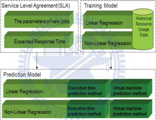
the minimum number of VM which can complete the new MapReduce job within the users’ expected time. The system architecture of this framework is shown in Fig. 3.1.

In service level agreement (SLA) module, users have to input the new input file, the execution parameters and the response time they expected. This information is sent to prediction model.

In training model, the system collects the historical resource usage data including the number of VM, execution parameters and execution time of old input files. In addition, regression-based model are adopted to train the historical usage data. The training model will output the model which has smallest RMSE to prediction model.

The historical resource usage data, the execution parameters of new jobs, the expected response time and the model which is output by training model are the input of prediction model. In prediction model, regression-based methods are adopted to predict the number of VM and execution time.

Chapter 4

RPF Algorithms

We propose two algorithms to predict the minimum number of VM of a MapReduce job. The details of two algorithms are shown in Section 4.1 and Section 4.2.

Algorithm 1 Training Algorithm

Input: S : {(s11, . . . , s1n, z1), . . . , (sk1, . . . , skn, zk)},a set of execution parameters and

execution time.

Output: A :{a1, . . . , am},coefficient set of regression equation. if LinearM odel then

Fill the set S in f (x1, . . . , xn, A) = a1x21+ . . . + anx2n+ an+1x1+ . . . + a2nxn+ am

Find out A to minimize∑k_i=1[zi − f(si1, . . . , sin, A)]2.

       f (s11, . . . , s1n, A) = a1s211+ . . . + ans21n+ an+1s11+ . . . + a2ns1n+ am f (s21, . . . , s2n, A) = a1s221+ . . . + ans22n+ an+1s21+ . . . + a2ns2n+ am · · · f (sk1, . . . , skn, A) = a1s2k1+ . . . + ans2kn+ an+1sk1+ . . . + a2nskn+ am else if N on− linearModel then

Fill the set S in f (x1, . . . , xn) = a1ea2x1 + . . . + a2n−1ea2nxn + am

Find out A to minimize ∑k_i=1[zi− f(si1, . . . , sin, A)]2.

       z1 = f (s11, . . . , s1n) = a1ea2s11 + . . . + a2n−1ea2ns1n+ am z2 = f (s21, . . . , s2n) = a1ea2s21 + . . . + a2n−1ea2ns2n+ am · · · zk = f (sk1, . . . , skn) = a1ea2sk1+ . . . + a2n−1ea2nskn+ am end if end if

4.1

Training Algorithm

Users have to execute the jobs whose input file is time-related or same with the new MapReduce job’s input file before executing RPF prediction process. The input of training algorithm are a set of execution parameters and execution time of these jobs,

S : {(s11, . . . , s1n, z1), . . . , (sk1, . . . , skn, zk)}. Because we use regression-based methods

to predict the minimum number of VM, the output of training algorithm is the coef-ficient set of regression equation, A : {a1, . . . , am}. There are linear and non-linear

regression model. In linear model, the set S is filled in f (x1, . . . , xn) = a1x21 + . . . +

anx2n+ an+1x1+ . . . + a2nxn+ am to find out the set A. Otherwise, the set S is filled in

f (x1, . . . , xn) = a1ea2x1+ . . . + a2n−1ea2nxn+ am to find out the set A in non-linear model.

4.2

Prediction Algorithm

Algorithm 2 Prediction Algorithm 1

1: Input: P : {p1, . . . , pn−1},a set of execution parameters, Regression Model, A :

{a1, . . . , am}, the set of coefficient of regression model, EP T :expected execution time 2: Output: N :number of execution VMs

3: for i := 1 to r do

4: if RegressionM odel = LinearM odel then 5: Fill the set A,set P and EP T in

6: f (x1, . . . , xn) = a1x21+ . . . + anx2n+ an+1x1+ . . . + a2nxn+ am

7: Use the following function to predict the number of execution VMs N .

8: N = f (p1, . . . , pn−1, EP T ) = a1s21+. . .+an−1sn2−1+anvi2+an+1p1+. . .+a2n−1pn+

a2nvi + am 9: else

10: if N on− linearModel then

11: Fill the set A ,set P and EP T in

12: f (x1, . . . , xn) = a1ea2x1 + . . . + a2n−1ea2nxn+ am

13: Use the following function to predict the number of execution VMs N .

14: N = f (p1, . . . , pn−1, EP T ) = a1ea2p1 + . . . + a2n−2ea2n−1pn−1 + a2nea2nvi + am

15: end if

16: end if 17: end for

After training procedure, the system predicts the minimum number of VM of the new job by prediction algorithm. The input are a set of execution parameters, P :

{p1, . . . , pn−1}, regression model, a set of coefficient of regression model which is the

The output is the minimum number of VM, N . The set of new execution parameters and the expected execution time are set to be the input of the regression model. After the regression process, the model outputs the minimum number of VM. The pseudo code of prediction algorithm is shown in Algorithm 2.

Algorithm 3 Prediction Algorithm 2

1: Input: P : {p1, . . . , pn−1},a set of execution parameters, Regression Model, A :

{a1, . . . , am}, the set of coefficient of regression model,V : {v1′, . . . , vr′},a set of testing

number of VM, EP T :expected execution time

2: Output: N :number of execution VMs

3: Let T :{t1, . . . , tr} be the set of predicted execution time responding to set V. 4: Let P RT : be the time in set T which is smaller than EPT and is the largest one in

T.

5: for i := 1 to r do

6: if RegressionM odel = LinearM odel then 7: Fill the set A,set P and set in

8: f (x1, . . . , xn) = a1x21+ . . . + anx2n+ an+1x1+ . . . + a2nxn+ am 9: Use the following function to predict the execution time ti.

10: ti = f (p1, . . . , pn−1, vi) = a1s21+ . . . + an−1s2n−1+ anvi2+ an+1p1+ . . . + a2n−1pn+

a2nvi + am 11: else

12: if N on− linearModel then

13: Fill the set A and set X in f (x1, . . . , xn) = a1ea2x1 + . . . + a2n−1ea2nxn + am 14: Use the following function to predict the execution time ti.

15: ti = f (p1, . . . , pn−1, vi) = a1ea2p1 + . . . + a2n−2ea2n−1pn−1 + a2nea2nvi+ am

16: end if

17: end if

18: Find the time PRT in set T which is smaller than EPT and is the largest one in T.

19: After finding PRT, we can know the index i and get the corresponding VM number.

20: end for

In some programs, the parallelization is not achieved very well. It causes that the number of VM is only related with the set of execution parameters or expected execution time. Therefore, we cannot predict the number of VM directly. We propose another methods to solve this problem. There are two steps in this proposed prediction algorithm. First of all, we use regression model to predict the execution time of the new job executed

N is the minimum number which can complete the new job with P :{p1, . . . , pn−1} within

the EP T . The pseudo code of prediction algorithm is shown in Algorithm 3.

The input are a set of execution parameters, P : {p1, . . . , pn−1}, regression model,

a set of coefficient of regression model which is the output of training algorithm,A :

{a1, . . . , am}, the expected execution time, EP T and a set of testing number of VMs,V :

{v′

1, . . . , vr′}. The output is the minimum number of VMs,N. There are two steps in

proposed prediction algorithm. First of all, we use regression model to predict the exe-cution time of the new job executed by different number of VMs and make up the set

T : {t1, . . . , tr}. The second step is comparing every execution time we predict with the

EP T and find out the time which is called P RT . P RT is smaller than EP T and is the

largest one in T . After finding P RT , we can output the VM number which is correspond-ing to P RT . The VM number, named N is the minimum number which can complete the new job with P :{p1, . . . , pn−1} within the EP T .

Chapter 5

Case Study

The data intensive jobs such as data mining jobs usually execute repeatedly by the same input files with different arguments. If users execute jobs in parallel, the execution time can be reduced intensively. While users rent the VMs to execute jobs in parallel, RPF enables users to use the least resource to execute parallel jobs. We demonstrate parallel frequent pattern growth (FP-growth) and parallel K-means on RPF to evaluate the per-formance of RPF. FP-growth is the most popular algorithm to analyze association rules from a lot of data. We modify FP-growth algorithm to parallel FP-growth algorithm which can execute on Hadoop platforms and collect the historical job usage data to esti-mate the fewest VM number of a new FP-growth jobs. The introduction of FP-growth is in Section 5.1.

5.1

FP-growth

A retailer such as Walmart may analyze the purchase relationship of products for product arrangement. They can execute FP-growth algorithm with different support which is the appearance frequency of products to find out the association rules of products. Therefore, the resource prediction of executing FP-growth with different support is really important. In addition, the input data of FP-growth such as the sales information of Walmart is huge. Executing FP-growth in parallel can reduce execution time massively. Therefore,

(a) The execution example of FP-growth

(b) The execution example of FP-growth on RPF

Case :

Support=1000 1200sec Support=1200 800 sec

Support=1500 600sec The number

of VMs

Expected execution time

Figure 5.1: The execution scenario of FP-growth.

min_support = 3

Customer ID Items bought Ordered

1 {a, c, d, f, g, i, m, p} {f, c, a, m, p} 2 {a, b, c, f, i, m, o} {f, c, a, m} 3 {b, f, h, j, o} {f, b} 4 {b, c, k, s, p} {c, b, p} 5 {a, c, e, f, l, m, n, p} {f, c, a, m, p} ID:1 {} f:1 c:1 a:1 m:1 p:1 ID:2 {} f:2 c:2 a:2 m:1 p:1 b:1 m:1 ID:3 {} f:3 c:2 a:2 m:1 p:1 b:1 m:1 b:1 ID:4 {} f:3 c:2 a:2 m:1 p:1 b:1 m:1 b:1 c:1 b:1 p:1 {} f:4 c:3 a:3 m:2 p:2 b:1 m:1 b:1 c:1 b:1 p:1 ID:5

Figure 5.2: Constructing FP-trees.

the execution time and execution status such as the number of VMs and support. This historical resource usage data can be used to predict the execution number of VMs.

5.1.1

Parallel FP-growth

FP-growth uses the divide and conquer strategy to find the frequent items. There are two phases in FP-Growth algorithm. First phase is constructing FP-tree. In this phase, we find frequent items whose appearance frequency is larger than minimum support and sort items in frequency descending order, Fig. 5.2. And then we construct a root node which is marked by null and add the branch of each traction. The second phase is FP-Growth. In this phase, we find out conditional pattern bases which are associated with every frequent

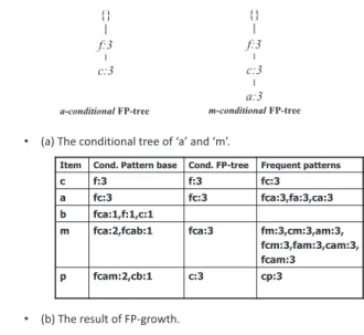
• (a) The conditional tree of ‘a’ and ‘m’.

• (b) The result of FP-growth.

Item Cond. Pattern base Cond. FP-tree Frequent patterns

c f:3 f:3 fc:3

a fc:3 fc:3 fca:3,fa:3,ca:3 b fca:1,f:1,c:1

m fca:2,fcab:1 fca:3 fm:3,cm:3,am:3, fcm:3,fam:3,cam:3, fcam:3 p fcam:2,cb:1 c:3 cp:3 {} f:3 c:3 a-conditional FP-tree {} f:3 c:3 a:3 m-conditional FP-tree

Figure 5.3: Conditional tree and result of FP-growth. ID Items 1 f a c d g I m p 2 a b c f l m o 3 b f h j o 4 b c k s p 5 a f c e l p m n Support=3 map reduce counting

ID Items 1 f c a m p 2 f c a b m 3 f b 4 c b p 5 f c a m p

Figure 5.4: MapReduce counting in Parallel FP-growth.

are put in conditional FP-trees. After constructing conditional FP-tree of every frequent item, we can output the frequent patterns, Fig. 5.3.

In parallel FP-growth, we execute MapReduce counting to find frequent items whose appearance frequency is larger than minimum support and sort items in frequency de-scending orderFig. 5.4. After MapReduce counting, frequent items are separated into many parts for every mapper to execute. Every mapper output the conditional patterns according to input files and send the result to the reducers. The reducers have two step to execute. First, the reducers collect the conditional patterns from every mapper and com-bine these patterns which are associated with same frequent item. Second, the reducers construct the conditional FP-tree of every frequent item and output the frequent patterns Fig. 5.5. The execution time of parallel FP-growth is much shorter than the execution

map reduce 1.{(c:3)} | p 2.{(f:3,c:3,a:3)}|m 3.{}|b 4.{(f:3,c:3)}|a 5.{(f:3)}|c f c a m p f c a b m f b c b p f c a m p map map map map p : f c a m m: f c a a : f c c : f m : f c a b m: f c a a : f c c : f b : f p : c b b: c p : f c a m m: f c a a : f c c : f

Figure 5.5: The execution process of parallel FP-growth.

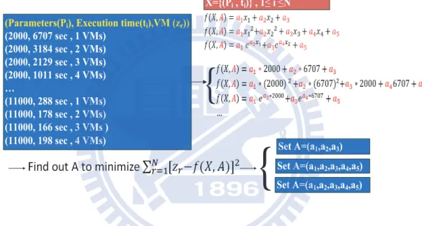
(Parameters(Pi), Execution time(ti),VM (zr))

(2000, 6707 sec , 1 VMs) (2000, 3184 sec , 2 VMs) (2000, 2129 sec , 3 VMs) (2000, 1011 sec , 4 VMs) … (11000, 288 sec , 1 VMs) (11000, 178 sec , 2 VMs) (11000, 166 sec , 3 VMs ) (11000, 198 sec , 4 VMs) Set A=(a1,a2,a3) Set A=(a1,a2,a3,a4,a5) Set A=(a1,a2,a3,a4,a5)

ż

ż

X={(Pi, ti)} , 1≤ i ≤N

Figure 5.6: The example of training algorithm by FP-growth.

5.1.2

Parallel FP-growth on RPF

We execute parallel FP-growth on map-reduce platform with different support. Therefore, we can collect different execution parameters, such as support and execution time to be the input of training algorithm. In Fig. 5.6, we input support 2000 to 11000 and the historical execution time in the training algorithm. After executing training algorithm, we can obtain an regression model whose root mean square error (RMSE) is the smallest. We use this regression model to predict the number of execution VMs for the new jobs. The new job’s support which is 5000 and expected response time 750 second which is set by users is the input of prediction algorithm. We put the support, the expected response time and the regression coefficient set A which is the output of training algorithm into the

X={(5000,750 sec)} 2.2455VM 3 VM Input:(5000,750 sec)+

Set A:{a1,a2,a3,a4,a5}={6.2883e-008, 2.7878e-007 , -0.0011 , -0.0026 , 8.1528}

Figure 5.7: The example of prediction algorithm 1 by FP-growth.

(support,#VM) X={(5000,1) Ƀ (5000,4)} (5000, 1VMs)->1389.9 sec (5000, 2VMs)->744.3 sec (5000, 3VMs)->409.2 sec (5000, 4VMs)->384.4 sec Expected 750 sec 2 VM

Input:(5000,750 sec)+

Set A:{a

1

,a

2

,a

3,

a

4,

a

5

}={0.000059843, 155.2 , -1 , -1111.2 , 5853.3}

Figure 5.8: The example of prediction algorithm 2 by FP-growth.

prediction equation. The equation outputs the fewest number of VMs. The example of prediction algorithm is shown in Fig. 5.7. If the prediction result is not accurate enough, we can try to use prediction algorithm 3 to estimate the number of execution VMs. We put the support, the number of VMs and the regression coefficient set A which is the output of training algorithm into the prediction equation. The equation outputs the execution time of every situation. We can use the expected execution time and the result of prediction algorithm to decide the fewest number of VMs of the new job. Fig. 5.8 shows the example of prediction execution time methods.

5.1.3

Parallel FP-growth on RPF Experiment Setup

We construct two physical machines as the platform. The CPU of physical machines is Intel(R) Core(TM) i7-2600 CPU 3.40GHz and 4G ram. There are four virtual machines in each physical machine. There are 1 core and 1G memory in each virtual machine. Hadoop is installed in virtual machines. We refer to [5] and Apache Mahout project [10] to modify the Fp-growth in parallel. The dataset is from [8]. We choose the dataset which

(a) The curve of linear regression.

(b) The curve of quadratic regression. (c) The curve of exponential regression.

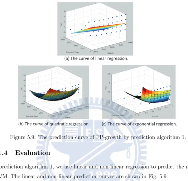
Figure 5.9: The prediction curve of FP-growth by prediction algorithm 1.

5.1.4

Evaluation

In prediction algorithm 1, we use linear and non-linear regression to predict the number of VM. The linear and non-linear prediction curves are shown in Fig. 5.9.

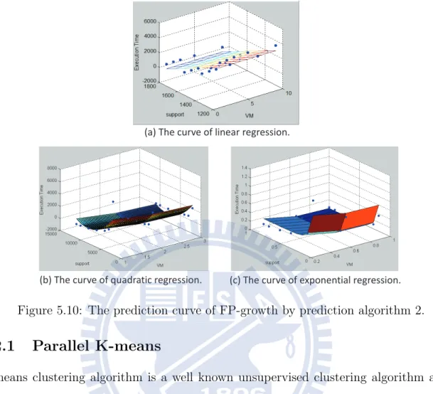
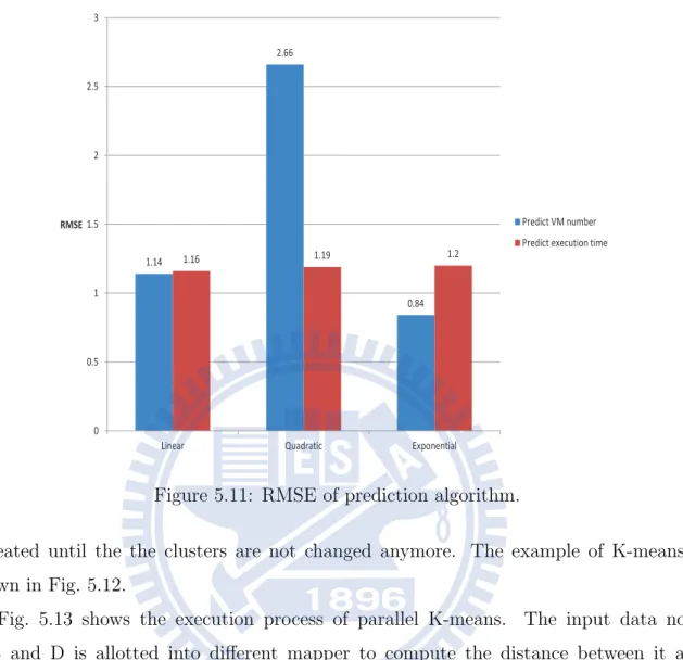
In prediction algorithm 2, we use linear and non-linear regression to predict the exe-cution time. The linear and non-linear prediction curves are shown in Fig. 5.10. Fig. 5.11 shows the RMSE of prediction algorithm 1 and prediction algorithm 2. We can see that the prediction result of exponential function is the most accurate and the result of quadratic function has the maximum error. Overall, the regression methods we propose can output the fewest number of execution VMs to users accurately.

5.2

K-means

K-means is the simplest cluster algorithm to find clusters from a lot of data. We modify K-means algorithm to parallel K-means, execute it on Hadoop platforms to collect the historical job usage data and estimate the fewest VM number of a new K-means jobs. The scenario and introduction of K-means is in Section 5.2.1.

(a) The curve of linear regression.

(b) The curve of quadratic regression. (c) The curve of exponential regression.

Figure 5.10: The prediction curve of FP-growth by prediction algorithm 2.

5.2.1

Parallel K-means

K-means clustering algorithm is a well known unsupervised clustering algorithm and it partitions objects into groups by analyzing the relationship or similarity of objects. Usu-ally, the input data of K-means called dataset is intensive. For example, the BigCross dataset [1] which is 11,620,300 points in 57-dimensional space and the Census1990 dataset [2] which is 2,458,285 points in 68 dimensions are used in [12]. Furthermore, analyzing the relationship between objects could be processed in parallel. The sequential K-means algorithm could be modified to a parallel K-means algorithm. Then, we use the parallel K-means to be a case study of RPF.

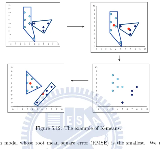
K-means is used to partition the data into K clusters. The input of K-means are the cluster number K and the data which is used to cluster. The output is K clusters. There are four steps of K-means. First step is choosing K data to be the central node of

1.14 2.66 0.84 1.16 1.19 1.2 0 0.5 1 1.5 2 2.5 3

Linear Quadratic Exponential

RMSE Predict VM number

Predict execution time

Figure 5.11: RMSE of prediction algorithm.

repeated until the the clusters are not changed anymore. The example of K-means is shown in Fig. 5.12.

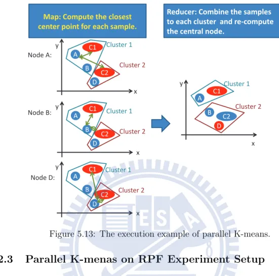
Fig. 5.13 shows the execution process of parallel K-means. The input data node A,B and D is allotted into different mapper to compute the distance between it and every central node C1, C2. After mappers output the distance result of A,B and D, the reducers have two step to execute. First, the reducers find the closest cluster for A,B and D according to the distance result. Therefore, B is changed to cluster 2. Second,the reducers recompute the central node of every cluster according to the average value of the data node in the clusters. The central node of cluster 2 is changed to D. The mapper and reducer process are iterative executed until the clusters are not changed anymore.

5.2.2

Parallel K-means on RPF

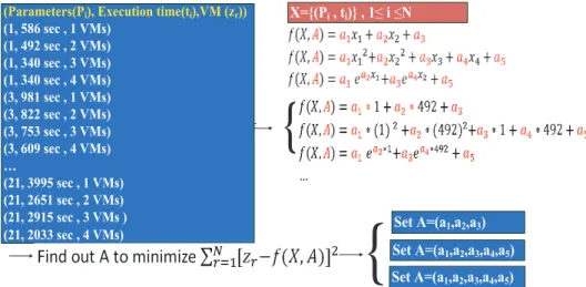
We execute parallel K-means on map-reduce platform with different K. Therefore, we can collect different execution parameters, such as K and execution time to be the input of training algorithm. In Fig. 5.14, we input k = 1, 3..., 21 and the historical execution

0 1 2 3 4 5 6 7 8 9 10 0 1 2 3 4 5 6 7 8 9 10 0 1 2 3 4 5 6 7 8 9 10 0 1 2 3 4 5 6 7 8 9 10 0 1 2 3 4 5 6 7 8 9 10 0 1 2 3 4 5 6 7 8 9 10 0 1 2 3 4 5 6 7 8 9 10 0 1 2 3 4 5 6 7 8 9 10

Figure 5.12: The example of K-means.

regression model whose root mean square error (RMSE) is the smallest. We use this regression model to predict the number of execution VMs for the new jobs. We input the new job’s K which is 10 and expected response time 2000 which is set by users in the prediction algorithm. We put the K, the expected response time and the regression coefficient set A which is the output of training algorithm into the prediction equation. The equation outputs the fewest number of VMs. The example of prediction algorithm is shown in Fig. 5.15. If the prediction result is not accurate enough, we can try to use prediction algorithm 3 to estimate the number of execution VMs. Fig. 5.16 shows the example of prediction execution time methods. We put the K, the number of VMs and the regression coefficient set A which is the output of training algorithm into the prediction equation. The equation outputs the execution time of every situation. Finally, we can use the expected execution time and the result of prediction algorithm to decide the fewest

x y A B D C1 C2 Node A: x y A B D C1 C2 Node B: x y A B D C1 C2 Node D: x y A B D C1 C2

Map: Compute the closest center point for each sample.

Reducer: Combine the samples to each cluster and re-compute the central node.

Cluster 1 Cluster 2 Cluster 1 Cluster 2 Cluster 1 Cluster 2 Cluster 1 Cluster 2

Figure 5.13: The execution example of parallel K-means.

5.2.3

Parallel K-menas on RPF Experiment Setup

The experiment environment is same with the FP-growth experiment. We refer to [15] and Apache Mahout project [10] to modify the K-means in parallel.The dataset is also same with FP-growth dataset which is rating data sets from the MovieLens web site [8]. We choose the dataset which consists of 10 million ratings and 100,000 tag applications applied to 10,000 movies by 72,000 users. We use K-means to cluster the users who have the same interest of movies.

5.2.4

Evaluation

In prediction algorithm 1, we use linear and non-linear regression to predict the number of VM. The linear and non-linear prediction curves are shown in Fig. 5.17.

In prediction algorithm 2, we use linear and non-linear regression to predict the exe-cution time. The linear and non-linear prediction curves are shown in Fig. 5.18. Fig. 5.19 shows the RMSE of prediction algorithm 1 and prediction algorithm 2. We can see that the prediction result of quadratic function is the most accurate and the result of linear

(Parameters(Pi), Execution time(ti),VM (zr)) (1, 586 sec , 1 VMs) (1, 492 sec , 2 VMs) (1, 340 sec , 3 VMs) (1, 340 sec , 4 VMs) (3, 981 sec , 1 VMs) (3, 822 sec , 2 VMs) (3, 753 sec , 3 VMs) (3, 609 sec , 4 VMs) … (21, 3995 sec , 1 VMs) (21, 2651 sec , 2 VMs) (21, 2915 sec , 3 VMs )

(21, 2033 sec , 4 VMs) Set A=(a1,a2,a3)

Set A=(a1,a2,a3,a4,a5)

Set A=(a1,a2,a3,a4,a5)

ż

ż

X={(Pi, ti)} , 1≤ i ≤N

Figure 5.14: The example of training algorithm by K-means.

X={(10,2000 sec)} 2.19VM 3 VM Input:(10,2000 sec)+

Set A:{a1,a2,a3,a4,a5}={-0.0061, 1.7929e-007 , 0.2494 , -0.0019 , 3.3953}

Figure 5.15: The example of prediction algorithm 1 by K-means.

function has the maximum error. We also can find that the RMSE of RPF is no more than 1.5. In brief, RPF can predict the fewest number of execution VMs to users accurately.

5.3

PSO

Particle Swarm Optimization (PSO), an optimization algorithm that was inspired by bird and fish foraging social behavior [4]. In the beginning, the birds have no idea about the food location. They guess and fly to better location by their experience and intuition. When a bird finds the food, it broadcasts the location to other birds. Other birds fly to the food location. Bird foraging behavior is the concept of mutual influence in society which can lead all individual bird toward the location of the optimal solution. PSO has become popular because it is simple, requires little tuning, and has been found to be

(K,#VM) X={(10,1) Ƀ (10,4)} (10, 1VMs)->2660 sec (10, 2VMs)->1909.6 sec (10, 3VMs)->1437.4 sec (10, 4VMs)->1243.5 sec Expected 2000 sec 2 VM

Input:(10,2000 sec)+

Set A:{a

1

,a

2

,a

3,

a

4,

a

5

}={-3.24, 139.1 , 162.3, -1167.7 , 2389.8}

Figure 5.16: The example of prediction algorithm 2 by K-means.

(a) The curve of linear regression.

(b) The curve of quadratic regression. (c) The curve of exponential regression.

Figure 5.17: The prediction curve of K-means by prediction algorithm 1.

5.3.1

Parallel PSO on RPF

The steps of resource prediction of parallel PSO is same with parallel FP-growth and parallel K-means. We execute parallel PSO with Rosenbrock s test function [9] which is defined following by different dimension d.

f (x) = d−1 ∑ i=1 [ (1− xi) 2 + 100(xi+1− xi2 )2] xi ∈ [−100, 100].

(a) The curve of linear regression.

(b) The curve of quadratic regression. (c) The curve of exponential regression.

Figure 5.18: The prediction curve of K-means by prediction algorithm 2.

algorithm. After the process of training, we predict the minimum number of VMs of a new job with different d by algorithm 2 or algorithm 3. The performance of parallel on RPF is shown below.

5.3.2

Parallel PSO on RPF Experiment Setup

The experiment environment is same with the FP-growth and K-means experiment. The input dataset is generated by latin hypercube sampling [6] with different domain. The optimization function of PSO is Rosenbrocks test function and xi ∈ [−100, 100]. We use

PSO to find optimal solution of Rosenbrocks function.

5.3.3

Evaluation

We use linear and non-linear to predict the number of VM in prediction algorithm 2. The curve of linear and non-linear prediction are shown in Fig. 5.20.

0.83 _0.8 0.92 1.155 1.08 0.96 0 0.2 0.4 0.6 0.8 1 1.2 1.4

Linear Quadratic Exponential

RMSE Random Predict VM number

Random Predict execution time

Figure 5.19: RMSE of prediction algorithm.

algorithm 2 is more accurate than algorithm 1. The reason is that parallel PSO program is not thorough parallel. That is, while users’ program is not fully parallel, algorithm 3 can provide better solution.

(a) The curve of linear regression.

(b) The curve of quadratic regression. (c) The curve of exponential regression.

Figure 5.20: The prediction curve of PSO by prediction algorithm 1.

1.07 1.22 1.09 0.92 0.99 0.99 0 0.2 0.4 0.6 0.8 1 1.2 1.4

Linear Quadratic Exponential

RMSE Predict VM number

Predict execution time

Chapter 6

CONCLUSION

In this paper, we proposed a resource prediction framework (RPF) to predict the mini-mum number of execution VMs which can execute the users’ jobs within a user specified response time. We not only proposed RPF but also demonstrated parallel FP-growth, parallel K-means and parallel PSO on RPF to evaluate the performance of RPF. The evaluation results showed that RPF can predict the number of VM accurately and can be adopted by data intensive algorithms. This is a big progress in resource provisioning field. In the future, we will propose a VM allocation model to combine with RPF which can make resource provisioning more accurately.

Bibliography

[1] The bigcross datasets. http://www.cs.uni-paderborn.de/en/fachgebiete/ag-bloemer/research/clustering/streamkmpp.

[2] A. Frank and A. Asuncion. Uci machine learning repository. http://archive. ics. uci.

edu/ml, 10, 2010.

[3] S. K. Garg, S. K. Gopalaiyengar, and R. Buyya. SLA-based Resource Provisioning for Heterogeneous Workloads in a Virtualized Cloud Datacenter. In IEEE International

Conference on Algorithms and Architectures for Parallel Processing, 2011.

[4] J. Kennedy and R. Eberhart. Particle swarm optimization. In Neural Networks,

1995. Proceedings., IEEE International Conference on, volume 4, pages 1942–1948.

IEEE, 1995.

[5] H. Li, Y. Wang, D. Zhang, M. Zhang, and E. Chang. PFP: Parallel FP-Growth for Query Recommendation. In Proceedings of the ACM conference on Recommender

systems, 2008.

[6] M. McKay, R. Beckman, and W. Conover. A comparison of three methods for selecting values of input variables in the analysis of output from a computer code.

Technometrics, pages 239–245, 1979.

[7] A. McNabb, C. Monson, and K. Seppi. Parallel pso using mapreduce. In Evolutionary

Computation, 2007. CEC 2007. IEEE Congress on, pages 7–14. IEEE, 2007.

[8] Movielens data sets. http://www.grouplens.org/node/7.

[9] J. Nelder and R. Mead. A simplex method for function minimization. The computer

[10] S. Owen, R. Anil, T. Dunning, and E. Friedman. Mahout in action. Manning Publications Co., 2011.

[11] G. Reig, J. Alonso, and J. Guitart. Deadline Constrained Prediction of Job Re-source Requirements to Manage High-Level SLAs for SaaS Cloud Providers. IEEE

International Symposium on Network Computing and Applications, 2010.

[12] M. Shindler, A. Wong, and A. Meyerson. Fast and accurate k-means for large datasets.

[13] F. Tian and K. Chen. Towards Optimal Resource Provisioning for Running MapRe-duce Programs in Public Clouds. In IEEE Conference on Cloud Computing, 2011. [14] P. Xiong, Y. Chi, S. Zhu, H. J. Moon, C. Pu, and H. Hacigumus. Intelligent

Man-agement of Virtualized Resources for Database Systems in Cloud Environment. In

IEEE International Conference on Data Engineering, 2011.

[15] W. Zhao, H. Ma, and Q. He. Parallel k-means clustering based on mapreduce. Cloud