Novel multiresolution metrics for content-based image retrieval

Novel Multiresolution Metrics

for

Content-Based Image Retrieval

Zheng-Yun Zhuang, Ming Ouhyoung

Wayne @ cmlab .csie.ntu.edu

.

tw,

ming

@ cmlab.csie.ntu. edu. tw Communications and Multimedia Laboratory, Department of

Computer Science and Information Engineering, National Taiwan University, Taipei, Taiwan

Abstract

This paper proposes three

new

ideas and

one

revision about

image

metrics and their applications.

Of

most

im-

portance

is

the multiresolution ‘shape metric ’, which measures distances according to images’ content shape information. Accompanied with it is

a

feature/non-feature image characterization philosophy. The second eflort is the modijication of an existing ‘color metric’, whose dis- tance computation is dominated by color distribution of images. The third idea is on analyzing image querying behavior of the general public,

so

as

to propose and de- sign

(a

versatile ‘power metric’, which holds the proper- ties of both the ‘shape metric’ and the ‘color metric’, for dealing with various kinds of hand-drawn queries. Fi-

nally, a f e r applying the ‘shape metric’ to

vdeo

shot boundary detection,

a

multiresolution scene change de- tection algorithm is proposed. For now, we have imple- mented these metrics on

a

personal computer for two

applications, one is for image database management with content-based indexing and the other is for video shot boundary detection. Experiments show that the speed and the accuracy of both image retrieval and

scene

change deteclion are quite well.

fiid that a better way to find a particular image on the Web is to provide content-based image retrieval(or in- dexing) and to maintain such a database periodically with a spider program. To date, however, there are only a few content-based image database systems that have already been developed, let alone applications on the Web. Our goal is to develop a system that can be extended for con- tent-based image search on the Web.

For our purpose, we design our image metrics with the feature extraction method in wavelet transform domain due to the fact that multiresolution analysis on images provides a good way to characterize images, to find the signature of images, and to catch the most significant information of them. Moreover, for properly designing these metrics, we had observed that in user hand-drawn image querying systems, a user may behave as an impres- sionist and emphasize on the color distribution in his query images while another one may like to give a sketch and draw the shape of her figure in monochrome. This makes us design our image metrics according to these two criteria. Therefore, the result includes three metrics. Shape metric computes the distance between images by their content shape information while color metric does by the color distribution information. Yet another one, the power metric, which is adjustable

and

is a mixture of the

above two, counts on both kinds of information.

I.

Introduction

1.2

Overview

1.1 NIotivation and Objective

As !he need of data mining on the Web grows, various kinds of search engines are developed. Search engines responsible for keyword indexing are now available and the telchnology is reliable. Of course, one may use the same itechnology to built a search engine that is responsi- ble for image searching by keywords. But if that were true, tl’le search engine would be very difficult to use, due to the fact that properties of images may not be suitably coded. There is no standard rule in the world for image naming. Besides, different image producers may give different names to the same image.

If we examine on this problem more closely, we will

In section 2, we will have theoretical discussions about the proposed metrics. Image metric concepts and some metrics that were proposed previously are discussed in section 2.1 and 2.2. Then we give in brief the definitions of our metrics and explain how they operate in section 2.3 without telling why. Section 2.4 reveals some observa- tions about the user behavior on producing a query image. Then section 2.5 explores the proposed metrics whereas 2.6 unveils the mechanism of the shape metric in more detail.

The system implementation of the proposed metrics is to be introduced in section 3 in short. Section 4 will show the experiments, benchmarks, and results about the met-

rics and the system. After that, we will move to the con- clusion, discussion, and future work in section 5.

1I.Proposed Adjustable Metric

2.1 Overview

To measure the distance between two images, we need a conceptual ruler or, a metric. For image search, the metric is used to compute the distance between the two characteristics of the query image and some target image in database. These distances are then sorted in order to form a queue that each queue member represents one image in database.

In our metric system, both the shape metric Ls and the color metric Lc are fixed. Only the power metric Lp, which is a mixture of the above two, behaves like a flexi- ble amoeba and can be changed on demand. However, it copes with all kinds of hand-drawn query images.

2.2 Existing Metrics

Some previous image metrics are intuitive and straight- forward. In the area of machine and robot vision, given two image planes A and B, probably the most obvious metrics used to measure the distance or error between the two images are the pixel difference metrics. These metrics in image processing usually cost a lot of time, especially the

L2

metric.

Recent researchers solve these problems by some fea- ture extraction techniques or some fast metria[ 1][3][4]

[ 5 ] . Some people find the similarity between images by histogram-based or DCT-intensity-based approaches. These might be suitable for those query images that were scanned but not so proper for hand-painted or drawn query. Others try to find a metric that counts primarily those types of differences that a human would use for discriminating images, but give less weight to the types of errors that a human might ignore for this task. Fortunately, such an image metric, associated with the multiresolution signal decomposition, has been proposed in [3] with their experiments in image querying. In the articles, that pro-

posed metric is called the Le metric. However, as we shall discuss, this metric deals with ‘painted query’ in major but may not cope with all the drawing behaviors of those who want to query.

2.3 Proposed

Metrics

2.3.1 Metric Definitions

Conceptually, our metric Lp is a dynamic mixture of Ls and Lc, where

Ls

is the ShapeMetric and Lc the Color-

Metric. Mathematically and globally, our Lp metric is defined

as:

where Ls is defined by:

(2.1) or equally,

while Lc is defined by:

(3) 13J

From the above definition, note that each one of A’ and B’ is some plane of the transform domain image (they are the transform domain images of source images A and

B).

We will use the word plane, or channel, to represent dif- ferent domains of an image rather than use the word do- main directly to avoid the ambiguity. In our system, after we have performed multiresolution 2-D

Haar

wavelet decomposition on an image, we can get the transform domain image of it. For each image plane, the transform domain representation of it contains one DC value in the upper-leftmost pixel(Plane[Ol[O]) and the other pixel values(Plane[i]lj] where i j # 0) are treated

as

coeflcients after transformation. These transform domain coefficients, together with the DC value, are more significant and may give more information to us than our source domain im- age pixels.

We adopted the standard Haar basis to be our decom- position basis for performing multiresolution wavelet transfomation. Although H a m Transform has poor com- pression ratio in signd coding[7], it is very fast and has been proved to be a good image feature extraction trans- form[2][3]. As we know, two-dimensional Haar trans- form(2-D

HT)

is an orthogonal transfoxm and is separa- bZe.[7] This means that we can perform a 2-D

Haar

trans- form on a 2-D image in two phases, with each phase be- ing composed of l-D Haar transforms.

The second point worth mentioning is that both

A“

and

A”‘

_{are the truncated and quantized version of}

_A‘,

which has been transformed, and so is it to

B”

and

B”.

What differs is the number of quantization levels. Coeffi- cient values in

A”

are of three quantization levels (-1, 0, 1) for the computation of Lc

as

was

suggested in [31, whereas those in

A”’

are of two levels (0, 1) for the computation of the Ls metric, as we shall discuss in the next sub-section. Besides, only metric Lc involves the DC value, which is proportional to the average density of the

source image plane, in the original transform domain plane. Ls considers nothing about DC values.

Third, the shape metric Ls is slightly different in con- text, but is very different in semantics from the color metric Lc, which is derived from the Le that we had re- ferred to. We will make this point clearer in section 2.6. The fourth and the last, our final L‘ is evidently a metric of mixture. Although there are no individual research outside our system made to prove the discriminating ca- pability of the metric Ls, which is responsible for finding shape-like images, we can see the ability of this metric in our query experiments by setting the parameter *i of L‘ mebk and in our scene change detection experiment where the Ls metric is applied.

2.3.2 Two-Level Feature/Non-feature Quantization

Here we list the quantization method mentioned in the previous discussion. The two-level quantization plane

A’”’

for the computation of Ls is obtained from quantiz- ing the transformed plane

A’

by the following formula.

A’”’

:

A’”

[

i]

[

j

] =

~ s s e ~ ~ ( ~ ; m k ~ ~ ~ ( ~ b s ( ~ ’ [ j ] [ j ] ) ) )

<MI)

(4)

Here Assert() is like the function that we use in pro- gramming languages. It evaluates the enclosed boolean expression then returns 1 if the expression is true or 0 otherwise. Rankof() is for selecting feature coefficients to be quantized as 1. This computation requires a sorting on coefficients in

A’

.

In the evaluation, transform domain coefficient with the largest magnitude has rank 1-st. A transform domain pixel whose rank is greater than k will become 0, which represents a non-feature coefficient, in the feature plane

A”

.

Note that the result feature plane is binary and it, in fact, can be obtained from

A”

by a non- standard “quantization” in integer domain as the follow- ing,

( 5 ) After the process, those transform domain coefficients with larger magnitudes, no matter they are positive or negative, are kept as 1. This speeds up the computation of distance measuring by our image metric L’, which in- volves a boolean non-equal test and will be discussed in the following paragraphs.

A”’

: A”’[i][j] =

( A ” [ i] [ j] l

2.4

User Behaviors on Image Querying

2.4.1 Classifications of Query Behavior

Consider if a subject without any training is asked for the first time to paint a query image, what the query im- age will be like? Correctly answering this question will

have great influence on the design of our metrics.

Now we start to analyze the behavior of those who want to query for a particular image. One may paint or draw the query by looking at the printed or thumbnail version of that image. One can also do this from his im- pression of that image. In the former case, which is called painted-querying in tradition, one may investigate a thumbnail list of database images and select one from them that he wants to query for, or he may look at the printed image on books, on newspapers, or the oil paint- ings on wall. In the latter case, often called memory- querying, one may have visited a fine art museum. Somewhat attracted by some painting, he may want to acquire a digital version after coming back home.

2.4.2 Paint or Draw: How a Query Image is Pro- duced?

Some researchers classified the querying behaviors into painted-querying and memory-querying, both kind of them were discussed in the previous section. They would often like to find different metrics for these two kinds of querying, ignoring the fact that the major difference lying behind the query behavior is his drawing

or

painting process instead of what he takes

as

his drawing reference. What we should argue here is that, in fact, no matter which kind of image one has used as his reference to paint his query, the key point is how he paint Uae query. That is, does he paint or draw the query? Or, does he draw with paint?

Do not be confused with the two words ‘paint’ and ‘draw’. Here we just use the two words to classify the drawing behaviors. Painting a query means to us6 some or more colors to compose a figure. That is just what the impressionists do. Blurring the focus and emphasis on color distribution and on light presentation make the pic- ture looks similar in different resolutions. On the contrary, drawing a query means to use a pen or pencil of one or a few colors(often the same color in various gray-scales) to sketch the borders or shapes of things in image. One may draw a query if he forgets the exact colors used in the picture to search for. Some people are color blinds or are just weak in distinguishing colors, which is exactly the case of the writer of this paper. Such kind of drawing query may help. Or sometimes there are images that are mainly composed of text. Drawing querying also plays a role for finding them.

Now the meaning of a ‘draw with paint’ query is thus well defined. This kind of query is the image that carries not only all or partial shape information but also all or partial color information that the user wants to express. Figure 1 demonstrates the two major kinds of queries classified by us.

adjustable and dynamic metric Lp, the two extremes are Ls and Lc. The L‘ can degenerate as Ls or Lc to meet the case that the query image is a pure drawn query or a pure painted one. It can also be a mixture of Ls and Lc by some percentage that can be used to deal with those ‘drawn with paint’ query images.

2.5 Exploring the Proposed Metrics

2.5.1 The Adjustable Metric Lp

In equation (l), ,? is just a floating value ranging from 0 to 1 that controls the percentage of the two solutes in our metric system, which are Ls and Lc. When it is reset to 0, the L‘ becomes Lc and discriminates images only by the color distribution information of them. Conversely, if it is set to 1, Lp becomes Ls and distinguishes images merely by the shape of the content objects.

Also, in our system, a user can adjust /z to a percent- age value whichever he wants between 0 and 1 if his query is ‘drawn with paint’. In this case, the user can tune a slider bar, which represents current ,? , to any percent- age value depending on how much shape information his query image carries against color information.

2.5.2 Color Metric Lc

Now let’s go further to the discussion of Ls and Lc. Our Lc is modified from Le, which also emphasizes on color distribution of query images. The major difference is on weight assignment.

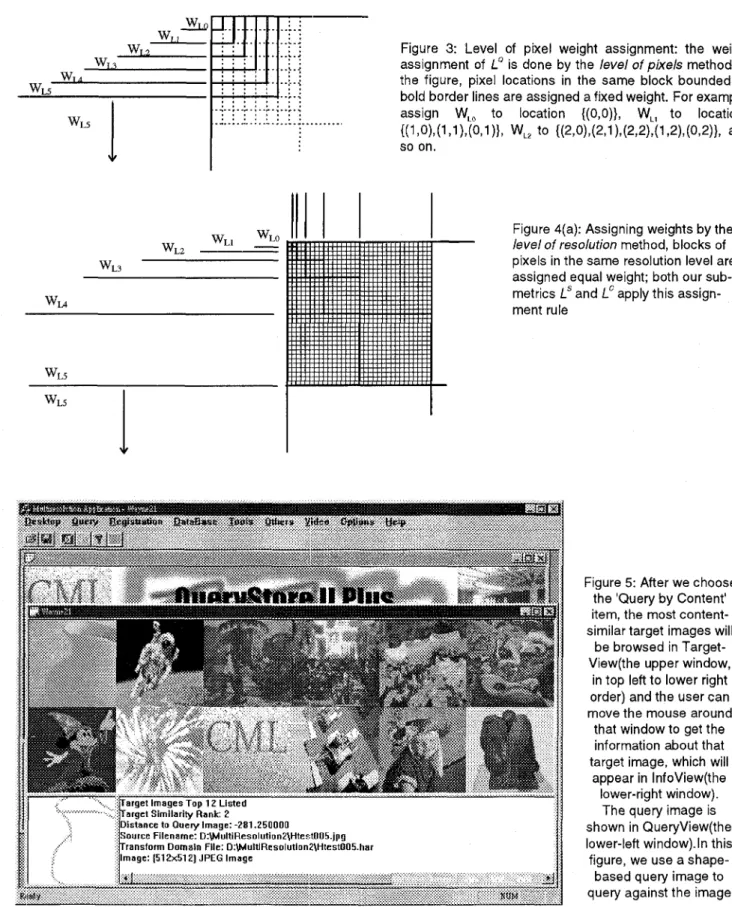
Both in Le and in our Lc, a specified weight is multi- plied to the DC difference and other weights are used as multipliers to those differences on truncated, quantized coefficients. Conceptually, these weights will form a weight table. The weight table derived from the formula of LQ, which is in level-of-pixel manner can be depicted in Figure 3 . But here we assign the weights according to level-ofresolution criteria rather than level-of-pixel. Ob- viously, our L“ uses the former but Le is according to the latter.

2.5.3 Level-of-Resolution Weight Assignment

As Figure 4(a) shows, we should refresh the weight ta- ble of Le with level of resolution shown in bold lines and re-assign values to the new table of Lc by averaging the original pixel weights in the same block. In this scheme, pixels are gathered into blocks and blocks of the same resolution level are assigned equal weights. This makes sense. The relation between the weight table entry

w Z j

with respect to transform domain pixel location (ij) and the weight that should be assigned to that table entry can be formulated in the following equation:

w .

. =

W, J,

where

n

=

Llw,

(max(

i,

j

))A

We would not like to re-experiment on obtaining the weights again because the weight table of Le has been experimented enough and proved to perform well. The result weight table of our Lc

is

as Figure 4(b) demon- strates. So far, we get our metric Lc from LQ by taking the same formula but assigning weights in different ways. What remains is the shape metric Ls whose weight as- signment is, surely, in level-of-resolution manner, too.

1.J

(6)

2.5.4 The Novel Shape Metric I?

Matching shapes of image contents has been a problem in robot and machine vision for a long time. Most re- searchers

try

to solve this problem by finding edge- detection algorithms, which may include sharpening edges, applying filters, enhancing contrast, convex-hull linking, and so on. This probably misleads a few people. Some people might believe that the shape-matching problem is equal to the edge-detection problem and think that the only way for finding shape-like images is to de- tect the edges efficiently first.

If we were designing our metric Ls by this way, it would not be so appropriate due to the extra computation time needed for edge detection and there is no time over- lap between performing multiresolution signal processing for L“ and performing edge detection for Ls. Thus we won’t try to find the solution in this way. Again, we use the abstraction ability of multiresolution signal decompo- sition. We just benefit from those truncated, quantized transform domain coefficients that has been computed during previous processes and at the same time has been used by Lc metric. This really utilizes the computation power and kills two birds with one stone.

2.6 Inside

Ls

The idea of Ls is simple from the equation. As we have mentioned, though the equation (2.2) for Ls is like the right-hand-side of the operand

‘+’

in Lc, the two metrics are by no means the same. To compare the Ls metric with Lc, consider the truncated and quantized coefficients A” in equation (3) and equation (2.2), which was written so

from the regular form (2.1) for comparison. Since there are only three levels in A”, only a few cases are possible for a given pixel. For clear realization of Lc, Ls and their difference, let’s consider a specified pixel location (ij) on two associated transformed plane A ” and B”. We can enumerate these cases and discuss how they will effect on the result distance computed by two metrics Lc and Ls:

B”[i][j]=-1 or A”[i][j]=O or B”[i][j]=O, this pixel means the same thing on both planes and contributes nothing to both met- ric.

(2) If A”[i][j]=l and B”[i][j]=O or A”[i][j]=O and

B”[i][j]=I or A”[i][j]=-I and B”[i][j]=O or A”[i][J]=O and

B”[i][j]=-l, then the pixel on one plane means there is a feature but that on another doesn’t. In both metric, these points contrib- utes to the distance exactly the weight value associated with its locartion on the weight table.

(3) We have discussed seven cases of the nine possible ones.

There are still two cases possible and these cases makes the two metrics greatly different. Consider A”[i][j]=I and B”[i][j]=-l

or A”[i][j]=-l and B”[i][j]=l. In Lc, the absolute value of

A ” [ i ] [ j ] - B ” [ i ] [ ~ ’ ]

will be 2. Such a pixel contributes

double of the weight to the metric distance. This implies that there are much dissimilarities on the two planes at this location, because the 1 in one plane means a large positive transform

domain value and the -1 in another means a very negative one.

This makes sense for the metric Lc from this point of view. But in L?,

IA”[j][j]l-IB”[j][i]l

will become 0, let alone the absolute value of it. This implies that, in Ls, this pixel means the same thing on both planes, instead of great dissimilarity. How this could happen??

If we inspect our signal decomposition process, which is the Haar transform, by a magnifying glass, we will find something surprising. This function, as we have men- tioned, performs 1-D Haar decomposition on a sequence of discrete signals.

Suppose we are going to decompose a 1-D signal sig- n a 1 [ 3 by Haar transform, we can see that, in fact, the transform can be divided into Zog,S passes, depending on the signal size S . The first pass deals with the whole sig- nal, repacks the signal, and then halves it into two parts. The second pass deals with the left-half that we are inter- ested in, while the third does with the left-half of the left- half, whose size is a quarter of the original Signal [

1

, andL so forth. During each step in a pass, the algorithm jus1 takes a pair of adjacent signal values, calculates their sum and difference, normalizes the results by a constant factor, and redistributes these values into two locations in two halves(or bands), to form a new signal.

The right half of the repacked signal stores the infor- maltion about differences of nearby signal values. These values, in 2-D, hold high frequency information repre- senting the edge appearances of the original image.

Turn back to our Ls right now. Consider there is a transformed plane pixel truncated and quantized as 1, and a pixel in the same location as -1 on another transformed plane. In our reasoning just discussed, at the specified location, there must be shape edges on both planes. Fur- thermore, there is exactly a negative gradient in the for- mer plane and there is exactly a positive gradient in the latter. This implies that here, in Ls, we treat both positive andl negative-gradient edges as the same. A pixel location

with great positive value in one transformed plane but with great negative value in another should contribute nothing to L‘ metric!

In the Ls metric, in fact, no matter the edge is of posi- tive or negative gradient, it is merely ‘an edge’ from our point of view. This reflects the fact that there are only two meaningful quantization levels in Ls but three in Lc.

Still two points worth noting are that we do not accu- mulate the DC difference to our shape distance measure- ment and that we only count on only Y-planes in Ls met- ric. The first point is obvious since our ShapeMetric Ls is a pure shape metric and it should not take any informa- tion about average intensities of each color channel. The second point is derived from the fact that human-sensible edges can be shown in gray-scaled Y-plane of an image and it, at the same time, saves a certain amount of com- putation time as well. Experimental results also shows that taking I, Q planes into account helps nothing. As we will see in the following chapters, our searching time is proportional to how much couples of Ls and Lc are com- puted, that is, how much database entries there are. While the growth of image database can not be avoided, this time saving on Ls becomes extremely critical.

We shall give an illustration to show the query by shape in Figure 2. Here we draw a query image by its content shape and want to search for that image in our database. If we purely use our Lc metric, which is a color- based one improved from traditional Le, we will get nothing but that image whose color distribution is alike. 2.7

Image Conversion Policy

In our model, there are at least two requirements on im- ages for 2-D multiresolution signal processing. First, the image should be square. Second, the width and height of the image should be power of 2. Since not all of the col- lected images are both square and power-of-2 sized, some conversion step must be taken before feeding image data into the Haar transform filter. To achieve this, different conversion strategies are adopted in our model for differ- ent components.

Area sampling has been a major technique used to pre- vent the aliasing effect[6][11]. In our query system, we would use the concept supported from area sampling. Suppose our source image size is WxH, the sampled im- age size is SxS. Then our S can be computed from:

(7) Taking the advantage of that our area-sampled image size is ‘the nearest 2 power size’ of the original one, we have devised a fast algorithm for computing it.1131

s

=

~ a w ( 2 , l l o g ,

(min(

w,~))])

The result is a system Querystore I1 Plus built on Win- dows 95, as was shown in Figure 5. There are currently two components in the system, PowerIQ(Power Image Querying) for image database management with content- based querying and SmartSCD(Smart Scene Change De- tection) for video shot boundary detection. The PowerIQ not only supports normal primitives of image database manipulation, such as image registration, deletion, on-line browsing, listing, and modification, but is capable of content-based image querying either by shape, by color, or, by both. Moreover, it provides the user a free-for- adjust metric and a comfortable query environment. An-

other component, SmartSCD, applies the shape metric and detects scene changes in video efficiently[l][2].

1V.Experiments and Results

4.1 Metric System Parametrization

There are several parameters controlling our metric system. The key parameter 2 of our metric Lp can be adjusted dynamically while the system is running and should not be fixed. Thus our purpose is to look for the weight table WS for shape metric

Ls

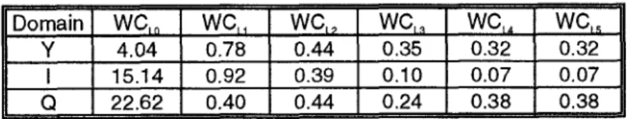
and the WC for color metric Lc. Besides, for both sub-metric, the number of topmost feature points to be considered(that is, how many transform domain coefficients with large magni- tudes should be selected after quantization) for both sub- metric is also a problem. Here we are going to give only 6 different weights for each channel according to level of resolution(Figure 4(a)).

As we have mentioned, our Lc is an improved version of Le, which takes 60 transform domain coefficients and its level-of-pixel weight assignment formula(by a func- tion called bin()) is modified to form our WC weight table(Figure 4(b)). Our Lc inherits its truncation(60 coef- ficients are considered) and quantization process (three levels) and uses our new level-of-resolution weight table. Thus our Lc performs well for ‘painted‘ queries that em- phasize on color distributions and at least as well as LQ does. What follows is finding the parameters for our shape metric Ls.

4.2 Derivation of the Weight Table

for

Metric L”

As we have discussed, the quantization process for Ls results in only two quantization levels. Then we must f i d out how many coefficients left after truncation, which is an integer t, are proper for our Ls metric and we should take an experiment for constructing the weight table WS for L’.

To make this experiment, 10 subjects were asked to

‘draw’ 30 shape-based query images and to Indicate which image he was searching for. Then we s m from t=60 to t=300(t must greater than 60 because the nature of shape-based images), taking 10 as a step unit. For each t, we train the weight table WS by the concept of prugres- sive refinement. For illustration, provided that we want to set up WS with its elements greater 0.0 and less than 20.0, and suppose we divide the range into four sub-ranges. We assign the weight of the multiresolution level 0 block@C) in WS(WSLo) as 0.0, level l(WSLl), 2(WSLz), 3(WSL3), 4(WSu) and 5(WSL5) as 2.5. Then we exhaustively iter- ate a 5-nested loop(which takes 45 times) by incrementing WSL1, WSLZ,

,..

, WSLs by 5.0 in each loop, and evaluate ‘the sum of rankings of the database images in relation to those queries’. Ideally, if

all

of the query images hit the topmost target(each time the first one in Targetview is exactly what the user searches for and the ranking of the image in that position is l), the sum of their rankings will be 30 and this is the lower bound. After the above loops, suppose we get a best weight table whose ‘the

sum

of rankings’ is the smallest with (WSLO,WSL~, WSLZ, WSW, WSU, WSLs)=(O.O, 7.5, 12.5, 7.5, 2.5, 2.5). Then we iterate the 5-nested loop again starting with (WSLo,WSL1, 0.625, 0.625). But this time the step amount is 1.25 to search for WSLl in [5.0,10.01, WSLZ in [10.0,15.01, W S L ~ in [5.0,10.0], and

so

on. Therefore we will find a better approximation of weight table WS by (WSu,WSLl, WSLz, WSL~, WSU, WSu) again.

For each t, we find the best total ranking and the asso- ciated weight table by iterating the 5-nested loop three times(3 training depth). The value on weight table is of precision 0.3125. As a result, we find that t=110 with the weight table shown in Figure 6 performs best.

WSu, WSL~, WSu, WSL5)=(0.0, 5.625, 10.625, 5.625,

4 3 System Benchmark

Our system was developed on Microsoft Windows 95 and can be executed from any PC. On such a platform, the amount of times needed for performing each of our processing steps individually were tested and summarized in Figure 7.

4.4 Experimental Results

For the validation of our metric syst

users were invited to paint 33 query images. He

or

she painted or drew their query images and

at

the same time answer our question “how much percentage of shape information does your query carry against color distribu- tion information”. We adjust our Lp according to his an- swer and search against the database. The result is as Figure 8 shows. In this table, the reader can see that the query behavior is going to be toward the two extremes.

That is, the query image either tends to emphasize on colior distribution, or does on shape expression.

V. Conclusion and Future Works

5.11

Conclusion and Discussion

13y making a survey on human behaviors of image que- rying, we have found that the major difference lying be- hind the query behavior is users'

drawing or painting

process.

We have argued that the key point is

how

he produces the query. Thus we classify the query images into three main classes, drawn query, painted query, or both.

To

cope with all these situations, we devise an ad- justable metric Lp which is a mixture of the two metrics Ls and Lc.

We have set up our color metric Lc for dealing with those painted queries. We assign the weight values on our weight table in a reasonable 'level-of-resolution' manner. Since there is another existing metric L ~ , also multireso- lution-based but in 'level-of-pixel' manner, that had been well tested for painted queries, we decide to obtain our Lc by reshuffling the weight table of Le into an improved 'level-of-resolution' one.

'ben we analyze those drawn query images and find that the key features of a drawn query are the shape edges. Unilike most previous approaches that is primarily by edge detection, we decide to match the shapes of two images in multiresolution transform domain. We also probe into the signal repacking process of wavelet de- coimposition and reveal that no matter the edge is of posi- tive or negative gradient, it is merely 'an edge' from our point of view. Therefore we propose a shape metric Ls with its two-level quantization feature extraction method- ology. In the meanwhile, experiments by simulation are maide to find out the proper weight table values for Ls, which are also organized in level-of-resolution, and to find proper numbers of coefficients to be kept as feature points.

Computation of each result metric takes just fractions of a second. Each

Ls

measurement cost only 0.00084 second while Lc is 0.00102. Thus each Lp takes 0.00187 in total to compute the distance between a pair of images. Therefore the metric computation time for searching against a 1000-images database is merely 0.84 second for

Ls,

1.02 for Lc, or 1.87 for Lp.

'Yet another point worth mentioning is that the. L' met- ric has been successfully applied to video scene change detection[ 1][2]. Unlike most previous detection operators, the L" metric not only detects scene change in multireso- lution transform domain, but also avoids regarding some shape-invariant video effects, such as fade-out or flash, as scene changes. We have now integrated this part into our

system.

5.2

Future

Work

Here we list some topics for our future research:

Automatic Metric Adjustment. In our current system, the adjustable parameter ,Iare free to adjust by the user. The user can adjust i t if one is not satisfied with current querying result and can adjust it toward any possible direction. We are going to let our system automatically find a 2 . To achieve this, several ideas may be considered. First, we could study the histo- gram of the query image. Therefore we would try to identify which class of query image does it belong to by the histogram. If the query image was a drawn one, often by two or a few high contrast colors, there would be only two or a few numbers of

peaks in its histogram. We could classify the query image ac-

cording to this clue. Alternatively, the systemmight also interact with the user each time before querying by bringing out the dialog for ,I adjustment. By this way, users could pre-set ,I

by his feeling of how much shape against color information did his query image carry. Yet another way is to provide candida- ture querying. Each time before the querying result is shown, the system computes the querying results by pure Ls and Lc. If either Ls or Lc is discriminate enough for current query image, the distances from the query image to the lS'-ranked target im- age and to the 2""dranked one should differ greatly. Thus we can select either Ls or Lc to be our default metric for this querying.

Further Metric Parameter Training. As we have indi- cated, the training depth of our current Ls metric is 3. That is, the precision of our current metric is 0.3125. There are two ways to improve our weight table further. The f is t way is to train more deeply and get a better precision of our weight table. The second way is to consider more than one weight table in each training. As we have mentioned, we use 'the sum of rank-

ings' to be our criteria for evaluating our weight table. We can set a threshold to filter these 'sum of rankings' and get more than only one weight table. A weight table that performs not so

good in depth n may perform well after training in depth (n+l).

That is, we give second chances to this kind of weight tables. Finding Hardware Solution for Ls. As we can see, since the featurelnon-feature characterization philosophy of Ls is

binary, the storage can be very small if we save the feature plane in our image database bit-wisely. Not only the feature plane extracted from the transformed plane are in binary form, but the computation of Ls involves boolean non-equal tests. This im- plies that, Ls distance measuring would be even faster and might be extremely fast if we have the dedicated hardware for compu- tation. The hardware can, of course, take two bit-wise stored feature planes A"' and B'", perform the non-equal tests simultaneously, and output the binary results to another feature plane, say C"

.

Then

c"

is used to mask another hard-wired plane, which represents the weight table. Taking an accu- mulation on the values of masked

D"

plane, we can obtain the distance easily. The entire process can surely be done in just a few clock cycles. Since the time overhead for transformation

and quantization is fixed and the growth of the image database can not be avoided, this acceleration becomes critical. Total distance measuring time for searching against a database with

10,000 images by Ls takes 8.4 second in current system but will be less than 1 second with hardware support.

Acknowledgement

We shall say special thanks to Chiou-Ting Xu, Kuang-Chih Lee, Hemg-Yow Chen, and Jia-Qiang He for the original idea about video application, for the paper re-organization, for the sugges- tion of video processing, and for the article support.

References

[I] Zheng-Yun Zhuang, Chiou-Ting Hsu, Hemg-Yow Chen, Ming Ouhyoung, Ja-Ling Wu, “Efficient Multiresolution Scene Change Detection by Wavelet Transformation”, Proceeding of E E E Intema- tional Conference on Consumer Electronics 97, pp.250-251 [2] Zheng-Yun Zhuang, Tzong-Jer Yang, Ming Ouhyoung,

“Multiresolution Scene Change Detection”, submitted to IEEE Transactions on Consumer Electronics

[3] Charles E. Jacobs, Adam Finkelstein, and David H. Salesin, “Fast Multiresolution Image Querying” ACM SIGGRAPH’95 Conference Proceeding, pp. 277-286, 1995

[4] Shiuh-Sheng Yu, Jinn-Rong Liou, and Wen-Chin Chen, “Computational Similarity Based on Chromatic Barycenter Algo- rithm” IEEE Transactions on Consumer Electronics, Vo1.42, No.2, [SI John S. Boreczky and Lawrence A. Rowe, “Comparison of Video Shot Boundary Detection Techniques”, Storage and Retrieval for Im- age and Video Database IV, SPIE 2670, pp. 170-199, 1996 [6] James D. Foley, Andries van Dam, Steven K. Feiner, and John F.

Hughes, “Computer Graphics: Principles and Practice” Addison Wesley, 1993

[7]Ali N. Akansu and Richard A. Haddad, “Multiresolution Signal Decomposition, Transforms, Subbands and Wavelets”, Academic Press, Inc, 1992

[XI Chiou-Ting Hsu and Ja-Ling Wu, “Multiresolution Mosaic,” IEEE Trans. Consumer Electronics, vol. 42, no. 3, November 1996, pp. 981-990

(91 Rafael C. Gonzalez, and Richard E. Woods, “Digital Image Proc- essing”, Addison Wesley

1101 Alan V. Oppenheim, Ronald W. Schafer, “Discrete Time Signal Processing”, Prentice Hall Inc, 1989

11 11 Alan Watt, Mark Watt, “Advanced Animation and Rendering Techniques” ACM Press, Addison Wesley, 1993

[I21 Adam Finkelstein, Charles E. Jacobs, and David H. Salesin, “Multiresolution Video” ACM SIGGRAPH’96 Conference Pro- ceeding, pp. 281-290, 1996

1131 Zheng-Yun Zhuang, “Efficient Multiresolution Image Characteri- zation Using Wavelet Transformation for Content-Based Image Re- trieval”, Master Thesis of National Taiwan University, 1997 1141 Alan L. Eliason, “System Development, Analysis, Design and

Implementation”, Harper Collins, 1990

[IS] Chiou-Ting Hsu and Ja-Ling Wu, “Hidden Digital Watermarks in Images,” under revised in IEEE Trans. Image Processing.

MAY 1996, pp. 216-220

--,

(b)

Figure 1: Two kinds of query images that a user tends to use. (a) a painted query image and its search target (b) a drawn query image and its target

(b)

Figure 2: Search(bottom4eft image) against our image database by a shape-based drawn query image (a) by color metric LC, which shows incorrect result, which is listed in the topleft corner (b) by shape metric LS, which shows correct result, top-left corner

Figure 3: Level of pixel weight assignment: the weight assignment of Lo is done by the level of pixels method; in the figure, pixel locations in the same block bounded by bold border lines are assigned a fixed weight. For example,

wL5

1

. . .

_.__

. . .

~ __.. .

.

._r..

. . .

.- ... . . ..-._ WLI

w,,

WLZ WL3

I

WL5

Figure 4(a): Assigning weights by the

level of resolution method, blocks of pixels in the same resolution level are assigned equal weight; both our sub- metrics LS and LC apply this assign- ment rule

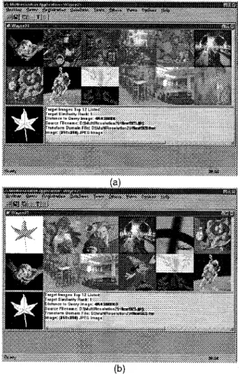
Figure 5: After we choose the 'Query by Content' item, the most content- similar target images will

be browsed in Target- View(the upper window,

in top left to lower right order) and the user can move the mouse around

that window to get the information about that target image, which will

appear in InfoView(the lower-right window).

The query image is shown in QueryView(the lower-left window).ln this figure, we use a shape-

based query image to query against the image

Figure 4(b): Values assigned to our WC weight table in level of resolution manner

Figure 6: The weight table of our shape metric LS: weight values are assigned in 'level of resolution' style, which was shown in Figure 5(a); we only assign five weights here because DC values(leve1 0 transform domain pixels) are not considered by our L', WS,, represents for the weight of level 1 coefficients, WS,, does for level 2, and so on

platform, an ordinary Pentium PC(133 Mhz). The unit of time is in second. This table also shows the properties of each step. For some step, if A property is 'yes', then the time is relative to the size of the query image. If B is 'yes', the time amount is effected by the size of current image database. If C is 'yes', that step is optional and may be omitted in some

Figure 8: Experimental Result: this table shows the hit rate of our testing query images drawn by 11 first-hand users; they are invited to paint or draw 3 query images and then asked 'how much shape information does each of your query image carry, or how much alike in color distribution is your query image with the target image?' The test database has 60 images and the result shows that our LP has a hit rate up to 88% if the top one choice is evaluated, and becomes 97% if we consider top 5% of candidate queue as reasonable search targets.