Robust real-time 3D trajectory tracking algorithms for visual tracking using weak perspective projection

Proceedings of the American Control Conference Arlington, VA June 25-27, 2001

Robust Real-time 3D Trajectory Tracking Algorithms for Visual

Tracking Using Weak Perspective Projection

Wei Guan Yau Li-Chen

Fu

and David Liu

'

Department of Electrical Engineering

Department of Computer Science and Information Engineering National Taiwan University, Taipei, Taiwan, R0.C.

2

Abstract

In

this

paper, motion estimation algorithms for the most general tracking situation are developed. The proposed motion estimation algoritbms are used to predict the location of target and then to generate a feasible control input so as to keep the target stationary in the center of image. The work differs from the previous algorithm of motion estimation in that it is capable to decouple the estimation of motion from the estimation of structure. The weak perspective projection is used to solve this problem. The modified optical flow is first calculated and then fed to motion estimation algorithms so as to generate an appropriate camera motion that achieve tracking. The important contribution of

this

work is that simple, numerically stable, none computation intensive, and correspondence-free 3D motion estimation algorithms are derived. A

visual

tracking system can be easily implemented

and

run

in real-time due to the simplicity of the proposed algorithms and thus increases their efficiency. The robustness and feasibility of the proposed algorithms has been validated by a number of experiments.

1. INTRODUCTION

Understanding the object motion is crucial to achieve the purpose of tracking. With

a

good knowledge of the object motion, one can improve the performance of tracking and thus increase its potential applications in machine vision systems. In

this

paper, we focus

on

the trajectory tracking

task

in general visual tracking system. Several experiments reported in [20], [13] revealed that their goal is only to pursue a moving target. However, the tracking problem to be solved in

this

research is not only to keep track of a moving target but also to locate the target at the image center of camera. Thus, the tracking problem to be investigated here is more challenging. In addition, the mathematical theory devised in

this

research is suitable to the most general tracking situation, i.e., three-dimensional (3D) target moving in three-dimensional space.

As we know, trajectory tracking or visual tracking is not a new research topic nowadays. Recently, several algorithms have emerged to handle

this

problem. In particular, the Interacting Multiple Model

(IMM)

algorithm for target tracking has received a lot of attention in [ll], [6], [9]. The IMM algorithm has been proved a very efficient and high performance algorithm for tracking the target [9]. However, several models are needed to account for the whole range target motion, which requires

considerable computational burden [ 1 81, [ 121. In addition, appropriately determine the number of models is crucial since increasing the number of models does not necessarily guarantee better performance [28].

For visual servoing in robotics, Hashimoto and Kimura have proposed an image-based or feature based method [29], [30], Espiau has developed the differential geometry approach [21], and Papanikolopoulos has introduced the adaptive control method [19]. Application of adaptive control in visual tracking is presented in [19], [14], [23], and [24]. As described in [19], the disadvantage of

this

approach is that the error will become si@icant when abrupt changes of the trajectories occur since the regulator cannot compensate for the abrupt changes fast enough.

Aloimonos and Tsakiris [3] have described a method which decomposes the tracking problem into two steps.

First, they estimate the motion parameters of the object. Second, they solve the minimization problem by using the estimation of the target motion parameter and then derive the desired rotational velocities of the camera that will achieve tracking. Their method however is based on the knowledge of the target shape and is subject to numerical instability problem.

The

methods described above

are in

complicated form or have their own drawbacks, which in turn increase the computational burden or deteriorate-s the tracking performance. Therefore,

this

paper proposes another close form solution for estimating the object motion during the tracking phase. This yields better performance

than

the previous methods. Recently, researches on the relationship between structure and motion have been widely conducted and have resulted in a variety of schemes for reconstructing motion for known structure [26], structure from motion [27], or both motion and structure [SI, [l]. Some researches

on

3D

space curves can be found in [22].

On

the other hand, research about the motion estimation is presented in [lo], [15]. Further, some motion understanding and trajectory planning which based on the Frenet-Serret formula are described in [4], [16], [17]. Using the knowledge of the motion and the structure, identification of the target dynamics may be accomplished. The organization of

this

paper is as follows: Section 2 outlines the procedure of designing the trajectory tracking algorithm. The implementation of these algorithms and the experimental results are presented in Section 3. Finally, conclusions are drawn in Section 4.

'

2. DESIGN OF TRAJECTORY TRACKING

ALGORITHM

We will make clear our main concept and notion for designing the trajectory tracking algorithm in this section.

Our goal here is to design a simple, none computation intensive, and numerically stable algorithm.

Our

main idea is that if the target motion is known, then the camera motion which will eliminate the relative motion of the target may be generated such that the tracking is achieved. In particular, if the motion of target is known well, then the “perfect tracking” may be achieved, i.e., image position of the target can always be kept at the center of image.

It is apparent that the estimation of the target motion is the first step in our proposed algorithm. In general, the motion of target is not known apriori. However, it can be estimated through the change of the image position which is called “optical flow” or image displacement. Using the observation of image displacement or optical flow which induced by target motion, one can estimate the motion of target if the camera is stationary. For the stationary camera and moving object, the optical flow induced by the target motion is:

where U, and v, are known as the optical flow or image

displacements and subscript

o

is denoted as object. If we assume a moving camera and a stationary object instead of a moving object and a stationary camera, then we can obtain the same result

as

(1) and (2) except for a sign reversal [19].

However it is not the case for the tracking phase since both the camera and target are moving during the tracking phase and therefore the optical flow is subject to both camera and target motion. In light of this observation, we must m o w the optical flow equation such that the optical flow is induced only by the target motion and irrelevant to the camera motion. Briefly, there are derived as follow. Suppose now that the optical flow at the time instant k during the tracking phase,is [U@), v(k)l’

,

then the optical flow is [ 191, [3]

44

= %(k) + u,(k) (3)

v(k) = v m + v“ (4)

where u(k) and v(k) are the total optical flow, u,(k)

and v,(k) are the optical flow induced by the target motion, whereas u,(k) and v,(k) are the optical flow induced by the tracking motion of the camera. Therefore, the optical flow induced by the target motion during the tracking phase can be obtained by modfymg (3) and (4) as follows:

U, (k) = u(k)

-

(k) ( 5 )

vo ( k ) = v(k)

-

vu (k) . (6)

Now, we would like to introduce our method of

finding this observable modified optical flow. Generally, the sum-of-differences

(SSD)

method is used to find the optical flow [19], [27]. Our method is different from

SSD

method since we have our own target detection algorithm as described in [7]. Using

this

target detection algorithm, the target image position can be obtained at any instant. Assume that the target image position is [x(k-i) y(ik-i)]’ at frame k

-

1 and our desired camera angular velocities are

q ( k - l ) = @ / A t and o y ( k - l ) = 6 J / A t , where At is the time interval between two consecutive frames,

4

is the pan angle and B is the tilt angle. Let the target move to the position [x(k) ,qk)]’ at the next m e , namely frame k,thenthe u ( ~ - i ) , ~ ( k - i ) , u,(k-i), ~ ~ ( k - 1 ) atfi-amek are derived as follows:

u(k - 1) = x(k) - x(k - 1)

(7)

v(k

-

1) = y ( k )

-

y ( k - 1) ( 8 )

.

x(k

-

l)y(k - 1) x2(k - 1) + f’ “ 9

u.(k

-

I) =(+I -x(k -1))

-[

0,(k -I)[

y )

- 0 J k - I)[

-)I

(1 1)

v#-l)=(u(k)-u(k-I))-

( ( A ’ L 1 1

o x ( k - l ) j(k-1)+p - 0 6 - 1 ) *(n-lly(k-D .(12) h o e e r practical way to obtain this modified optical flow is as follow:

u,(k -I) = x(k)

-

x(k -I) + (x+(k -I)

-

xo) ₍₁₃₎

v,(k

-

1) = Y ( k ) - r(k

-

1) + (YpndLt(k

-

1) - Y o ) (14) where x,,, y, are the image center and +(k-1) and ~ ~ ( k - 1 ) are the predicted target image position.

We can then estimate the target motion by using the modified optical flow. Two motion estimation algorithms are proposed here. The first motion estimation algorithm consists of estimation of translational velocity and rotational velocity, namely “full motion model” whereas the second algorithm composes only of estimation of translational velocity, namely “modest motion model”. Motion estimation task becomes peculiarly Micult in trajectory tracking since neither the structure (depth) nor the target motion is known. Accordingly, we propose a novel motion estimation algorithm which is independent of the estimation of structure. In other words, our algorithm is capable to decouple the estimation of motion fi-om the estimation of structure. Thus, the structure (depth) need not be

known

or estimated before solving the motion estimation task. To this end, the weak perspective projection [8], [2], [25] is used to alleviate this problem. The weak perspective projection model gives a good approximation when the size and the depth variation of the object are small compared with the distance between the object and the camera [25]. Details of theoretical error analysis of using this approximation model have been omitted for the sake of brevity and can be found in 173.

Suppose we are in frame

k

and we are now ready to estimate the target motion by using the modified version of optical flow.

First,

we abbreviate (l), (2) to the discrete time expression as

where

The matrix J ( x ( k - I ) , y ( k - l ) , Z ( k -1)) is called the image Jacobian and T=[T,

T

l-r and o = [y my U,]' E %' is the translational and rotational velocity.

Let

x,

=[,re U, 2 ~ 7be the reference point and this

point can be arbitrary chosen at either the center or the tip of area of the target. In order to keep the target's center coincident with the image center, the center of area of the target is thus chosen as reference point. The edge points which lie around

this

reference point are chosen as the feature points. Combining N feature points [XI

yly,

...

,

cXN

,,,,r

in (15) and using the weak perspective projection

model

[A,

yields,

1

IWl

Rewrite (1 7) as

C=GV

where e is the drsplacement or optical flow induced by target motion, G is composed of the feature's image coordinate and focal length and v consist of depth as well as translational and rotational velocities of the target with respect to the camera coordinate system. Specifically, matrix G and vector e depends only on observable quantities whereas vector v contains the quantities whch we want to estimate. In particular, for

N

= 3 , it will be proved in Theorem 1 shown below that the matrix G is nonsingular, and hence (18) can be easily solved as follow: v = G-'c

.

(19)

Theorem 1

: The matrix G is nonsingular if and only if three distinct, noncollinear feature points

p1

yI1r,

[x2 y21T, [x, y31T satisfy the following condition x,

;

j * o .

1:

Y2

$+Y? x,'+Y,'

q2+K1

Proof: Please see [7].

Remark

In particular, the above condition is easily satisfied by any three distinct points.

Let

then T(k-I) is obtained

as

follow:

For the modest motion model, we assume that the translational velocity dominates the rotational velocity given that the sampling time is short enough for two consecutive image frames. Therefore, we restrict ourselves to estimate the translational velocity due to the above assumption. In

this

way, (1

5)

can be simplified as:

Similar

to the full motion model presented previously, combining

N

feature points 14 yIlr,

...

,

pN yNy in (21) and using the weak perspective projection model, yieIds,

Then

This is not surprising for solving (23) by using the least- squares fonnulation:

Specifically, we show

that

the

matrix

is invertiile if and only if at least two of the N feature points are in distinctive image position. This will be revealed in Proposition 1.

Proposition

1: The matrix (PA) is invertible if and only if at least two of the N feature points are in distinctive image position.

b = H a . (24)

a = (HTH)-'HZb (25)

Proof: See

[q.

Using (25), T(k-1) is obtained as follows: T(k

-

1) = 8

The second step in our proposed algorithm is prediction. The prediction task is to predict where the target image location in W ek will 'move to' in the next frame k + l

.

It is easy to extract the image displacement at frame

k

by using the following equation if T(k) = T(k

-

1)

,

co(k) =co(k - I ) , and Z ( k ) = Z ( k

-

1) for the short sampling time.

where (x,,y,) is the target's centroid coordinate in image plane.

Thus, the prediction can be obtained as follow:

x,(k + I) = x,(k) + U#) (28)

Y,(k + 1) = Y , ( k ) + % ( k ) . (29)

This value is fed to the tracking module to generate the desired camera motion which will achieve the goal of tracking.

The last step is tracking. The tracking task is generate an accommodated pan and tilt angle so that the image center coordinate [x, y,]' will be coincident with the target coordinate y l ~ r after the pan and tilt movement.

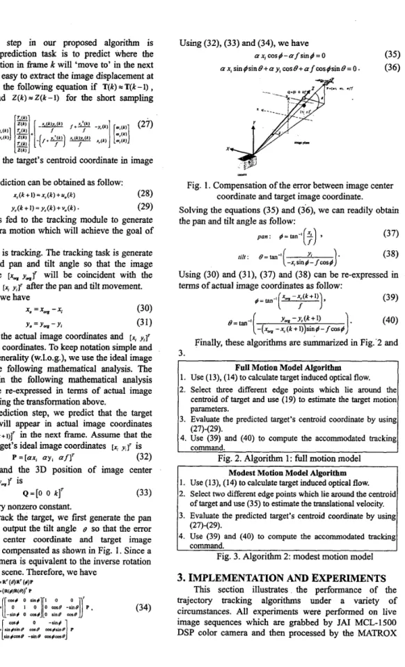
From Fig. 1, we have

x, =x- -x, (30)

(31)

Y . = Y , - Y ,

where [xo y , ~ r is the actual image coordinates and [x, y,lr

is the ideal image coordinates. To keep notation simple and without loss of generality (w.l.o.g.), we use the ideal image coordinate in the following mathematical analysis. The equations used in the following mathematical analysis obviously can be re-expressed in terms of actual image coordinates by using the transformation above.

From the prediction step, we predict that the target image position will appear in actual image coordinates [.. y , ] r = [ x , ( k + i ) y c ( k + l ) ] r in the next fiame. Assume that the

3D position of target's ideal image coordinates [x, ,,lr is where a = z , / f and the 3D position of image center coordinates [x, y,jr is

where k is arbitrary nonzero constant.

In order to track the target, we first generate the pan angle 4 and then output the tilt angle B so that the error

between image center coordinate and target image coordinate can be compensated as shown in Fig. 1. Since a rotation of the camera is equivalent to the inverse rotation of the point in the scene. Therefore, we have

-(R(+vwJ)' P P = [ a x , ay, af]' (32) Q = [ O 0 k]' (33) Q = R' ($)It' (+)P =[[ -w(

:'

;

o

s:6]p

-4 o :e rlne

-.,i).,

-e

.

(34) cm( 0 -nn(

Using (32), (33) and (34), we have

a x , cos4-afsin 4 = 0

(I xi sin (sin B+ a y , cos B+ af cosdsin B = 0 .

(35) (36)

Fig. 1. Compensation of the error between image center coordinate and target image coordinate. Solving the equations (35) and (36), we can readily obtain the pan and tilt angle as follow:

p a n : @=tan-'[:) 9 (37)

@ = m y x A k + l )

,

(39)

f

I

(38)

Using (30) and (31), (37) and (38) can be re-expressed in terms of actual image coordinates as follow:

-x, sin # yi - f cos#

1.

tilt : e= tan-'(

1.

(40) U, - U c ( k + l )

[

-( x, -x,(k + 1))sinl - f c o s b @=tan-'

Finally, these algorithms are su"arized in Fig..2 and

3.

Full Motion Model Algorithm 1. Use (13), (14) to calculate target induced optical flow. 2. Select three different edge points which lie around the

centroid of target and use (19) to estimate the target motion parameters.

3. Evaluate the predicted target's centroid coordinate by using 4. Use (39) and (40) to compute the accommodated tracking

Fig. 2. Algorithm 1: full motion model (27)-(29).

command.

Modest Motion Model Algorithm 1. Use (13), (14) to calculate target induced optical flow.

2. Select two different edge points which lie around the centroid of target and use (35) to estimate the translational velocity.

3. Evaluate the predicted target's centroid coordinate by using

4. Use (39) and (40) to compute the accommodated tracking (27)-(29).

command.

Fig. 3. Algorithm 2: modest motion model

3.

IMPLEMENTATION

AND

EXPERIMENTS

This section illustrates the performance of the trajectory tracking algorithms under a variety of circumstances. All experiments were performed on live image sequences which are grabbed by

JAI

MCL-1500 DSP color camera and then processed by the MATROX

f ID.

1

.am

.pD.-

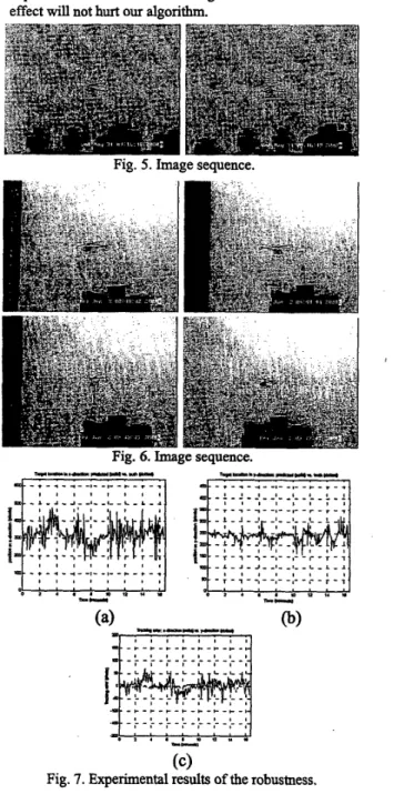
0 Robustness

Figure 6 shows the image sequence in which the rotation motion dominates the translational motion. For the rotation motion which dominates the translational motion, the target will change the pose, and this will yield the error in the computation of optical flow. However, the experimental results shown in Fig. 7 demonstrate that this effect

w

i

l

l

not hurt ow algorithm.

I I # I O , , I , , , , , , , I , , , , ! s - - - L - 4 - - 1 - - L - - L - J - - 1 -

-

n u - - - n - - - a - - l - - L

-

- 1 - -I-.. J

-

-

-

-:-

-

-;- -;

-

- f

-

-;-

-

-;-

-

+

-

-

a -, ,

, - - ~

I ,- _ , _ - , ,

- - , - -

,

fa---:--:--,

, , ,

,

. _ _ , _ - _ ( _ _ . _ _ _ _ , _ _

~ - - ~ - -

I , I I I I , - I - - - I - - + --.--,-- -4

--.--

, , , , I , ,

Fig. 5. Image sequence.

4. CONCLUSIONS

most general tracking situation are developed. The contribution of

this

work is that simple, none computation intensive, correspondence-free and numerical stable 3D motion estimation algorithms

are

developed. An important factor for the successful application of the extremely simple algorithms is based on the use of weak perspective projection model. The trajectory tracking algorithm based on these proposed motion estimation algorithms provides accuracy of the prediction of the trajectory of the maneuvering target.

The

proposed algorithms have been implemented in our visual tracking system [7]. Experimental results show that the proposed algorithms are accurate, robust, and feasible. In addition, all the experiments were done in the real-time. The potential of the proposed methods has been demonstrated by the presenting experimenbl results. We believe that the simplicity and the robustness of the proposed approaches can be applied to other general visual tracking system.

REFRENCES

[l] G. Adiv, “Determining Three-Dimensional Motion and Structure fiom Optical Flow Generated by Several Moving Objects,” ZEEE Trans. Pattern Analysis and Machine Zntelligence, vol.

PAMI-7,

no. 4, pp. 384-401, Jul 1985.

[2] J. Y. Aloimonos, “Perspective Approximations,” I m g e and Vision Cbmputing, vol. 8, no. 3, pp. 179-192, Aug 1990.

131 J.(Y.) Aloimonos and D. P. Tsakiris, “On the visual‘ mathematics of tracking,” Zmge and Vsion Computing, vol.

9, no. 4, pp. 235-251, Aug 1991.

[4] J. Angeles, A. Rojas, and C.

S.

Lopez-Cajun, “Trajectory Planning in Robotics Continuous-Path Applications,” IEEE

J. Robotics and Automation, vol. 4, no. 4, pp. 300-385, Aug

1988.

[5] A. Azarbayejani and A. P. Pentland, “Recursive Estimation of Motion, Structure, and Focal Length,” ZEEE Trans. Pattern Analysis and Machine Intelligence, vol. 17, no. 6,

pp. 562-575, June 1995.

[6] Y. Bar-Shalom, K. C. Chang and H. A. P. Blom, “Tracking a Maneuvering Target Using Input Estimation Versus the Interacting Multiple Model Algorithm”, IEEE Trans. on Aero. and Electro. Sys., vol. AES-25, no. 2, pp.

,

Mar 1989.

171 W. G. Yau, “Design and Implementation of Visual Servoing System for Realistic Air Target Tracking,” Master’s thesis, Dept. Elec. Eng., National Taiwan University, 2000.

[8] Andrew Blake and Michael Isard, Active Contours, London :

Springer-Verlag, cl 998.

[9] H. A. P. Blom and Y. Bar-Shalom, “The Interacting Multiple Model Algorithm for Systems with Markovian Switching Coefficients”, ZEEE Trans. Automatic Control, vol. 33, no. 8, [lo] S. Soatto, R. Frezza, and P. Perona, “Motion Estimation via Dynamic Vision,” ZEEE Pans. Automatic Control, vol. 41,

no. 3, pp. 393-413, Mar 1996.

[ll] K. J. Bradshaw, I.

D.

Reid, and

D.

W. Murray, “The Active Recovery of 3D Motion Trajectories and Their Use in Prediction,” ZEEE Trans. Pattern Analysis and Machine Intelligence, vol. 19, no. 3, pp. 219-233, Mar 1997.

[I21 W. S . chaer, R. H. Bishop, and J. Ghosh, “A Mixture-of- Experts Framework €or Adaptive “an Filtering,” ZEEE Trans. @stem, Man. and Cybernetics-Part B: Cybernetics,

pp. 780-783, Aug 1988.

vol. 27, no. 3, pp. 452-464, June 1997.

[13] N. Sawasaki, T. Morita, and T. Uchiyama, “Design and Implementation of High-speed Visual Tracking Systems for Real-Time Motion Analysis,” Z E E E Int. Con$ Pattern Recognition, vol. 3,478433,1996.

[14] L. Chen and S . Chang, “A Video tracking system with adaptive predictors,” Pattern Recognition, vol. 25, no. 10,

[15] Z. Duric, J. A. Fayman, and E. Rivlin, “Function From Motion,” IEEE Trans. Pattern Analysis and Machine Intelligence, vol. 18, no. 6, pp. 579-591, June 1996.

[16] Z. Duric, E. Rivlin, and A. Rosenfeld, “Understanding the Motions,” Image and Computing, vol. 16, pp. 785-797, 1998.

[17] Z. DuriC, A. Rosenfeld, and L. S . Davis, “Egomotion Analysis Based on the Frenet-Serret Motion Model,” Proc. ZEEE 4th Int. Con$ Computer Vision, pp.703-712, April [18] M. Efe and D. P. Atherton, “Maneuvering Target-Tracking With an Adaptive Kalman Filter,” Pmc. 37th ZEEE Con$ Decision & Control Tampa, Florida, pp. 737-742, Dec 1998.

[19] N. P. Papanikolopoulos and P. K. Khosla, “Adaptive Robotic Visual Tracking: Theory and Experiments,” IEEE Trans. Automatic Control, vol. 38, no. 3, pp. 429-445, Mar 1993.

[20] M. W. EMund, G. Ravichandran, M. M. Ttivedi, and S . B. Marapane, “Adaptive Visual Tracking Algorithm and Real- time Implementation,” Proc. IEEE Znt. Con$ Robotics and Automation, pp. 2657-2662, 1995.

[21] B. Espiau, E Chaumette, and P. Rives, “A New Approach to Visual Servoing in Robotics,” Z E E E Trans. Robotics and Automation, vol. 8, no.3, pp. 313-326, June 1992.

[22] 0. Faugeras and T. Papadopoulo, “A Theory of the Motion Fields of Curves,” Int. J. of Computer Vision, vol. 10, no. 2,

[23] J. T. Feddema, C. S. G. Lee, “Adaptive image feature prediction and control for visual tracking,” IEEE Trans. *stems, Man and Cybernetics, vol. 20, no. 5, pp. 1172-

[24] J. T. Feddema, C. S . G. Lee, “Adaptive image feature prediction and control for visual tracking with a moving camera,” Proc. IEEE Znt. G n J Systems, Man and Cybernetics, pp, 20-24, NOV 1990.

[25] T. Otsuka and J. Ohya, “Real-time Estimation of Head Using Weak Perspective Epipolar Geometry,” ZEEE FVorkshop on Application Computer Vision, pp. 220-225, 1998.

[26]

D.

B. Gennery, “Visual Tracking of Known Three- Dimensional Objects,” Int. J. Computer Vision, vol. 7, no.

[27] L. Matthies, T. Kanade, and R Szeliski, “Kalman Filter- based Algorithms for Estimating Depth from Image Sequences,” Znt. J. Computer Vuion, vol. 3, pp. 209-236, 1989.

[28] X. R. Li, and Y. Bar-Shalom, “Multiple-Mael Estimation with Variable Structure,” IEEE Trans. Automatic Control,

vol. 41, no. 4, pp. 478-493, April 1996.

[29] K. Hashimoto, T. Ebine, and H. Kimura, “Visual Semohg with Hand-Eye Manipulator

-

Optimal Control Approach,” IEEE Trans. Robotics and Automation, vol. 12, no. 5, pp. [30] K. Hashimoto, T. Kimoto, T. Ebine, and H. Kimura, “Manipulator Control with Image-Based Visual Servo,”

Proc. IEEE Znt. Con$ Robotics & Automation Sacramento, California, pp. 2267-2272, Apr 1991. pp. 1171-1180, Oct 1992. . 1993.. pp. 125-156,1993. 1183, Sept-Oct 1990. 3, pp. 243-270, 1992. 766-774, Oct 1996.