國 立 交 通 大 學
環 境 工 程 研 究 所
碩 士 論 文
三維非均質含水層污染源的推求
Identification of Contaminant Source in
Heterogeneous Aquifers
研 究 生:劉 易 璁
指導教授:葉 弘 德
三維非均質含水層污染源的推求
Identification of Contaminant Source in
Heterogeneous Aquifers
研 究 生:劉易璁
Student:Yi-Tsung Liu
指導教授:葉弘德
Advisor: Hund-Der Yeh
國立交通大學
環境工程研究所
碩士論文
A Thesis
Submitted to Institute of Environmental Engineering
College of Engineering
National Chiao-Tung University
in Partial Fulfillment of the Requirements
for the Degree of
Master of Science
in
Environmental Engineering
July, 2006
Hsinchu, Taiwan
中 華 民 國 九 十 五 年 七 月
三維非均質含水層污染源的推求
研究生:劉易璁 指導教授:葉弘德
國立交通大學環境工程研究所
中文摘要
本研究利用污染源鑑定模式 SATS-GWT,針對提升三維非均質含水層污染
源的鑑定案例與機率,分別利用蒙地卡羅模擬(MCS)與 Latin Hypercube Sampling (LHS)分層取樣法進行分析。在模擬污染擴散在非均質水力傳導場址時,首先以 模擬退火演算法進行場址條件模擬,產生一組具有固定平均值、標準偏差、和空 間 相 關 係 數 的 隨 機 非 均 質 水 力 傳 導 係 數 場 , 作 為 真 實 污 染 場 址 , 並 以 MODFLOW-GWT 模擬得到採樣觀測濃度值。為了分析監測井數目對提升污染源 鑑定機率的影響,第一個案例利用蒙地卡羅方法,在與先前相同的水文地質參數 條件下,進一步產生另外50 組不同的水力傳導場址,透過 SATS-GWT 模式來進 行污染源位置的推求。第二個案例則利用LHS 分層取樣法,LHS 方法是一種統 計取樣方式,透過LHS 方法對 1000 組非均質場址做取樣,並與第一個案例的結 果做比較。另外,第三個案例比較了五種不同監測井的採樣位置對於鑑定機率的 影響。因此,針對各案例的模擬結果,我們提出在所設計的三維非均質含水層場
Identification of Contaminant Source in
Heterogeneous Aquifers
Student : Yi-Tsung Liu Advisor : Hund-Der Yeh
Institute of Environmental Engineering
National Chiao Tung University
ABSTRACT
This study presents the analyses of contamination source identification probability in three-dimensional heterogeneous aquifers. A source identification model SATS-GWT is used to estimate the source information using Monte Carlo simulation (MCS) and Latin Hypercube Sampling (LHS) method. In the process of the source release simulation in the heterogeneous conductivity field, the computer program sasim, developed based on simulated annealing simulation and available in GSLIB, is first used to generate a random conditional hydraulic conductivity fields with a given mean, standard deviation, and correlation structure parameters. The measured concentrations at sampling points are simulated by MODFLOW-GWT with the assumed release concentration at known source location.
probability, the sasim program is used again to produce 50 realizations of random conductivity fields with known conductivities at some locations as conditioning data. The model SATS-GWT is applied to the contaminated site with one of the random conductivity fields to estimate the source information. Then the probability of obtaining the correct results can be estimated based on those 50 runs of Monte Carlo simulation (MCS). In addition, Latin Hypercube Sampling (LHS) method is also used for 50 conductivity fields drawn from a total of 1000 samples. Finally, a study is made to explore the effect of sampling location patterns on source identification probability. The simulated results regarding to the number of sampling points and the patterns of the sampling location for effectively determining source location in three-dimensional heterogeneous aquifers are concluded.
誌
謝
能夠完成這本碩士論文並且來到「寫致謝」這一扇門,是我在兩年前想都 不曾想過的一件事,感謝眾人群策群力的支持,僅以此文表達我心中的誠摯感謝。 首先感謝指導教授葉弘德老師,在我原本混亂的世界、沒有章法的大腦裡 開出一條大道,兩年的學習生涯從求學問到做事的態度、生涯規劃,不僅傳授了 許多寶貴經驗使我獲益良多,甚至到最後一刻還為了如何妥善的表達論文內容而 不厭其煩的悉心指導,才使論文能順利完成。另外,也感謝中國技術學院陳主惠 教授、台灣大學童慶斌教授、台灣大學劉振宇教授、美國中佛羅里達大學葉高次 教授四位口試委員的提點和寶貴意見,使論文更加完整。 感謝環工所最優秀的地下水研究室群,最有智慧但是事情老是多到做不完 的智澤學長、在家裡被兩個小孩子煩到學校還要被我煩的郁仲學長、永遠很有自 信每每扮演我的及時雨現在人在美國happy 的彥禎學長、環工所最漂亮聰明的雅 琪、彥如、嘉真學姊,以及兩年的夥伴淇汾同學、AOC 戰友定裕同學、兩位最 可愛講話很有趣然後時常穿高跟鞋ㄎ一ㄎ一ㄎㄡㄎㄡ的學妹敏筠和毓婷,為我的 碩士班生活留下許多豐富的回憶。 感謝與我從大學共戰至今的土木系同學,118、120、125 的所有室友,認識 你們真的很開心,以及創價學會所有一直鼓勵我陪伴我的大哥大姐和夥伴,六年 來在交大和你們一起努力所流下的汗水和淚水,是我人生最豐富的資產也是這輩 子最值得珍惜的情誼。最後,將此論文獻給我的家人,感謝父母在我低潮的時候
給予我包容,舅媽對我的親切照顧,佼盈的陪伴和充滿熱情的鼓勵,才能助我堅 持下去完成碩士班學業。當然還有所有幫助我、關心我的親戚朋友們,雖然你們 一定看不懂而且也不會想看我的論文,不過我真的很謝謝你們。 易璁 謹致於 交通大學環境工程研究所 2006 年 8 月
TABLE OF CONTENTS
ABSTRACT... III
TABLE OF CONTENTS...VII
LIST OF TABLES... VIII
LIST OF FIGURES ... IX
NOTATION ... X
CHAPTER 1 INTRODUCTION...1
1.1 BACKGROUND...1
1.2 LITERATURE REVIEW...2
1.2.1 Monitoring Well Design ...2
1.2.2 Latin Hypercube Sampling...4
1.3 OBJECTIVES...5
CHAPTER 2 METHODOLOGY ...6
2.1 GEOSTATISTICAL PROGRAMS:SASIM...6
2.2 GROUND-WATER FLOW AND TRANSPORT MODEL...7
2.3 SOURCE INFORMATION ESTIMATION MODEL :SATS-GWT ...7
2.4 MONTE CARLO SIMULATION...11
2.5 LATIN HYPERCUBE SAMPLING...11
CHAPTER 3 RESULTS AND DISCUSSION...14
3.1 HYPOTHETIC SITE DESCRIPTION...15
3.2 SCENARIO 1:EFFECT OF THE LEVEL OF AQUIFER HETEROGENEITY...16
3.3 SCENARIO 2:APPLICATION OF THE LHSMETHOD...20
3.4 SCENARIO 3:EFFECT OF SAMPLING POINT PATTERNS...23
CHAPTER 4 CONCLUSIONS ...26
LIST OF TABLES
Table 1 The measured concentrations and hydraulic conductivities in monitoring wells
for MCS method ...31
Table 2 Results of source identification for MCS method as σy = 0.5 (m/day) ...32
Table 3 Results of source identification for MCS method as σy = 1.0 (m/day) ...33
Table 4 Results of source identification for MCS method as σy = 1.5 (m/day) ...34
Table 5 The measured concentrations and hydraulic conductivities in monitoring wells for LHS method ...35
Table 6 Results of source identification for LHS method as σy = 0.5 (m/day)...36
Table 7 Results of source identification for LHS method as σy = 1.0 (m/day)...37
Table 8 Results of source identification for LHS method as σy = 1.5 (m/day)...38
Table 9 The measured concentrations and hydraulic conductivities in different sampling patterns as σy =0.5 (m/day)...39
Table 10 Results of source identification versus sampling location patterns as σy = 0.5 (m/day)...40
LIST OF FIGURES
Fig. 1. Flowchart of SATS-GWT. The OFVCALO represent the objective function
value of local optimal solution at candidate location...41 Fig. 2. The procedure for identifying source location along with the MCS method ...42 Fig. 3. The procedure for identifying source location along with the LHS method ....43 Fig. 4. The aquifer system with an area of 1000m by 1000m and the locations of real
source S1, eight suspicious sources near S1, and sampling points A to Q ....44 Fig. 5. The performance curves of the probability versus σ =0.5 (m/day) ...45 y Fig. 6. The performance curves of the probability versus σ =1.0 (m/day) ...46 y Fig. 7. The performance curves of the probability versus σ =1.5 (m/day) ...47 y Fig. 8. The cumulative frequency distribution of 1000 conductivity fields data of σy
= 0.5, 1.0, and 1.5 (m/day)...48 Fig. 9. The performance curves of the probability versus σ =0.5 (m/day) ...49 y Fig. 10. The performance curves of the probability versus σ =1.0 (m/day) ...50 y Fig. 11. The performance curves of the probability versus σ =1.5 (m/day) ...51 y Fig. 12. The performance curves of the probability versus sampling location patterns
NOTATION
lnK : Logarithm hydraulic conductivity y
σ : Standard deviation of the natural logarithm of hydraulic conductivity
y : The mean of the natural logarithm of hydraulic conductivity
λ : Correlation length
n : Number of sampling points
N : Number of simulation runs
M : Total number of conductivity fields
I : Total number of the interval of random values
i : The number of intervals
j : 1/I
NS :
Number of the ial solutions of release period and concentration generated at a candidate location
NT : Number of candidate location generated at one temperature
x : Trial solution
x’ : The neighborhood trial solution
f(x) : Objective function value of x f(x’) : Objective function value of x’
PSA : Acceptance probability of the trial solution x’
Te : Current temperature
est i
C, : Simulated concentration estimated at ith sampling point
obs i
CHAPTER 1 Introduction
1.1 Background
Most of significant threats to groundwater of various contamination sources include industrial landfills, regulated hazardous waste sites, underground storage tanks, and abandoned waste sites. More recent reports indicate that the soil and groundwater once contaminated, the tillage and health of inhabitant nearby the site may be influenced. Thus, when the contaminated site is announced, the remediation is imperative to act; yet, remediation is a complex and lengthy process. The difficulties arise from the uncertainty of aquifer characteristics and the contaminant source location in the landfill. The uncertainty of aquifer characteristics affects the results of predicting the groundwater flow and contaminant transport. The uncertainty of the source location makes the contaminant zone difficult to delineate or assess; moreover, the liability of the contaminant site is not easy to determine if the responsible parties of the contaminant site are several. In addition, large degree of variation in the hydraulic conductivity field may make the shape of the plume irregular, and consequently the source location becomes more difficult to detect. Thus, how to effectively increase the chance of source location identification is deserved further studies if the source location is unknown and the aquifer formation is
heterogeneous.
1.2 Literature Review
1.2.1 Monitoring Well Design
Among the methods of monitoring well network design in the literature, Meyer and Brill (1988) presented a method along with Monte Carlo simulation (MCS) for locating wells in a monitoring network to provide detection of contaminant plumes. Their method utilized two linked models, a simulation and an optimization model. The simulation model utilized an analytical solution to estimate the solute transport information. The optimization model offered the optimal placement of wells location. The Monte Carlo technique was used with the simulation model to reduce uncertainty effect of the contaminant concentration distribution. The result showed that the selected well network could detect the plume distribution effectively. Bagtzoglou et al. (1992) proposed an approach using particle methods and MCS to estimate the source location and time history in a heterogeneous aquifer. They analyzed two heterogeneous aquifers with perfectly known conductivity fields and conditioned conductivity fields. Twenty MCS runs were used in each case with different observation numbers. The results indicate that when 60 wells are used for the designed case, source identification with conditional conductivity field performs
as well as the simulation with perfectly known conductivity field. Meyer et al. (1994) proposed a further study about monitoring network design to detect the groundwater contamination distribution. They considered the resolution of multiple conflicting objectives: minimizing the number of wells in the network, maximizing the probability of detection, and minimizing the expected area of contamination at the time of detection. The design method, an extension of Meyer and Brill (1988), can be used to predict the appropriate number and location of monitoring network.
Storck et al. (1997) presented an uncertainty analysis incorporating the Monte Carlo method and the particle-tracking model for the monitoring well network to detect the leak of the groundwater contamination. The monitoring network optimization method extended the approach of Meyer et al. (1994) and applied in three-dimensional heterogeneous aquifers. They considered three conflicting objectives and applied their method to analyze an existing landfill site. The result revealed that their method worked for detecting the groundwater contaminant leak.
Mahar and Datta (1997) applied the nonlinear optimization model in identifying unknown pollution sources and used finite differences method to simulate the physical processes of transient flow and transport in the groundwater systems. They formulated the source estimation problem as a constrained optimization form and solved the objective function by nonlinear programming. In their study, the source
information for flow in steady or transient state was successfully identified. Recently, Chang and Yeh (2005) proposed a monitoring well design optimization method and developed a new model called SATS-GWT to identify the contaminant information. The model combines the simulated annealing, tabu search and three-dimensional groundwater flow and solute transport model MODFLOW-GWT, which was developed by the USGS. The proposed approach was employed to investigate the optimal number of sampling points and conditions for effectively estimating contaminant source information in three-dimensional homogeneous aquifers. They also suggested a guideline to allocate the sampling point location.
1.2.2 Latin Hypercube Sampling
Numerical simulation for the real world problems is often faced with a large number of simulation runs. Latin Hypercube Sampling (LHS) method can be applied to reduce the number of MCS method required. Mckay et al. (1979) first proposed LHS as an alternative method to random sampling. They compared three sampling methods, including LHS, simple random sampling, and stratified sampling, and associated estimators of the mean, variance, and the population distribution function of the model output. The results obtained from LHS appeared to be more precise than the other two types of sampling methods.
technique to analysis the sensitivity of subsurface stormflow parameters. In their study, the LHS could largely reduce the computational requirements in typical Monte Carlo uncertainty analysis and risk assessment. Zhang et al. (2003) applied the LHS method to compare with three random field generation algorithms: sequential Gaussian simulation available in GSLIB, the turning-bands method, and LU decomposition. The result showed that the LHS method gives a minimum deviation of the variance and it preserves the marginal distributions of the simulated variables. By using LHS in their study, the computational effort needed in solving groundwater flow and transport models was greatly reduced.
1.3 Objectives
This study has three objectives. The first objective is to investigate the relationship between the number of sampling points and the chance of the source identification using MCS in different characteristics of groundwater sites. The second objective is to use LHS instead of MCS in source identification and compare the results with those of MCS. The third objective is to study effect of patterns of sampling location on the source identification results.
CHAPTER 2 Methodology
2.1 Geostatistical Programs: Sasim
Random field generators were usually employed to produce realizations for representing field hydraulic conductivity or other physical properties with preserving some statistical parameters such as the mean, standard deviation, and correlation length. Among the process of simulating a field, which honoring the specific locations and preserving the variability is called conditioning simulation. Statistically, conditioning simulation with the actual field data can eliminates the deviation. Generating conductivity field with assigned field values at certain specific locations may lead to more accurate simulations. The geostatistical software library GSLIB (Deutsch and Journel, 1998) provided several random field generators which are capable of modeling spatially-correlated and conditional fields.
In this thesis, the program sasim is employed for generating a conditional conductivity field which has the total number of finite difference grid points of 25 x 25 in x and y coordinates. The conductivity fields are treated as heterogeneous and
isotropic in the horizontal plane. The basic idea of this program is to perturb continuously an original initial field and generates a required field. For generating heterogeneous and isotropic conductivity fields, four steps are taken: (1) generate the initial random field by the routine RNLNL of IMSL (2003) with specific field mean
and variance in which the variance is a histogram objection function, (2) choose the exponential model for the variogram and given the correlation range for the conductivity field, (3) set the weights of component objective function are one, (4) define the mechanism of perturbation and annealing schedule temperature to produce the required fields.
2.2 Ground-Water Flow and Transport Model
The groundwater model MODFLOW-GWT is developed by the United State Geology Survey. This model is based on a three-dimensional method-of-characteristics solute-transport model (MOC3D) (Konikow et al. 1996) and the modular three-dimensional finite-difference ground-water flow model, MODFLOW-2000, (Harbaugh et al. 2000), to simulate three-dimensional spatial and temporal plume distribution and ground flow field, respectively. The MODFLOW-GWT can simulate the groundwater flow and contaminant transport simultaneously. It also can handle steady and unsteady flows in an irregularly shaped flow system in which the layers can be the confined, unconfined, or combination of confined and unconfined aquifer.
2.3 Source Information Estimation Model : SATS-GWT
SATS-GWT. It combines the simulated annealing (SA), tabu search (TS) and three-dimensional groundwater flow and solute transport model MODFLOW-GWT.
The algorithm of SA is a useful and effective tool in determining optimal parameters of the objective function. In SA, an initial guess x is used to evaluate the
objective function value f(x). For any point x, a neighborhood trial solution x’ is
randomly generated and the objective function value of x’ is denoted as f(x’). These
values are using to solve the minimization problem, if f(x’) is smaller than f(x), then x’
is accepted and the current optimal solution x is replaced by x’. If f(x’) is not smaller
than f(x), then the Metropolis criterion is used to test the acceptability of the trial
solution. The Metropolis criterion provides a mechanism to accept inferior solutions and the acceptance of inferior solutions avoids the trial solution becoming trapped in a local. For solving minimization problem, the Metropolis’ criterion is given as (Pham and Karaboga 2000) > − ≤ = ) ( ) ' ( , ) ) ' ( ) ( exp( ) ( ) ' ( , 1 x f x f if Te x f x f x f x f if PSA (1)
where PSA is the acceptance probability of the trial solution x’ and Te is current
temperature.
In addition, the advantages of TS are learning and memory. The purpose of the tabu list is to memorize some lately evaluated trial solutions and to avoid trapping solutions in a local optimum. At the iterative process of TS, an initial guess for the
unknown variables is first assumed as the current solution (CUS) and be used to calculate the global optimal objective value (GOOV). Several adjacent candidate solutions (CASs) are generated and evaluated their objective values in the neighborhood of the current solution. For estimating the minimization problem, when the best objective value (BOV) is less than GOOV, the best CAS from the tabu list (TL) will be removed if it is in the list. Besides, the CUS is moved to the TL, and the best CAS becomes the new CUS and the BOV becomes the new GOOV. When BOV is larger than GOOV, the next best CAS will be selected if the best CAS is in the TL; otherwise, the best CAS becomes the new CUS. The procedures are repeated continually by generating other adjacent CASs from the neighborhood of the new CUS and stop until the stopping criterion is satisfied.
Based on the advantages of the SA and TS, both two methods are combined to estimate the source information which includes the source location, release period, and concentration. Besides, the model MODFLOW-GWT is used to simulate the groundwater flow and contaminant transport. Figure 1 shows the flowchart of SATS-GWT. This approach is employed to find the source information such as the source location, source release concentration, and release period. The objective function defined in their approach is to minimize
∑
= − = n k obs i est i C C n f 1 2 , , ] [ 1 (2)where Ci,est is the simulated concentration at the ith sampling point, Ci,obs is the
measured concentration at the kth sampling point, and n is the number of sampling
points. Eq. (2) is used to calculate the objective function value of the trial solution generated by the approach.
In SATS-GWT, the initial objective function value is calculated based on the initial guesses which include the source location and a constant value of release period and release concentration. The guess location for the source is considered as current location and TS is active to generate the source locations, called candidate locations. At each candidate location, SA generates NS trial solutions for the release period and concentration magnitude. For each set of trial solutions, the MODFLOW-GWT is employed to calculate the simulated concentrations at monitoring wells. The least value of the objective function among NS trial solution is considered as the objective function value at the candidate location (OFVCALO) and
the solution is considered as the local optimal solution. Then the TS method is used to estimate the global optimal objective function value. The number of candidate location generated in TS process at a temperature is defined as NT. After NT candidate locations are generated, the temperature is reduced with the specified reduction factor. The algorithm is terminated when the differences of the objective function value are less than 10-6 four times successively. The estimated source
information like source location, release concentration, and release period to the latest upgraded object function value is considered as the final solution.
2.4 Monte Carlo Simulation
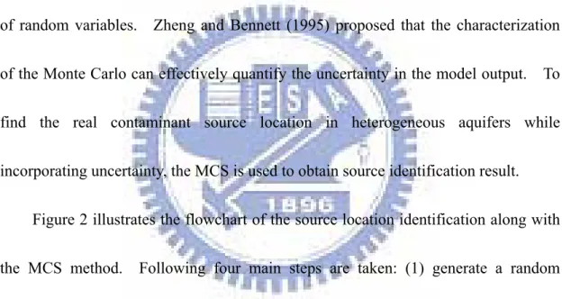
The MCS is a straightforward approach to generate a large number of equally likely random realizations, and it is widely used to analyze uncertainty associated with complex numerical models. It bases on the stochastic approach and knowledge of random variables. Zheng and Bennett (1995) proposed that the characterization of the Monte Carlo can effectively quantify the uncertainty in the model output. To find the real contaminant source location in heterogeneous aquifers while incorporating uncertainty, the MCS is used to obtain source identification result.
Figure 2 illustrates the flowchart of the source location identification along with the MCS method. Following four main steps are taken: (1) generate a random conductivity field conditioning on the known conductivity data, (2) simulate the contaminant plume distribution in a heterogeneous aquifer, (3) generate N conductivity fields using sasim, and (4) identify the source information.
2.5 Latin Hypercube Sampling
The LHS method was first introduced by MacKay and Beckman (1979) in an effort to reduce the required computational cost of purely random sampling
methodologies. It can be viewed as a compromise sampling method that incorporates the desirable features of random and stratified sampling methods and can obtain more stable outcomes than random sampling method. The advantage of the LHS approach is to ensure that the selected samples can be properly cover entire sample space. It is generally recognized as one of the most efficient size reduction technique.
To obtain N LHS conductivity fields, following six steps are taken: (1) generate M random conditioning conductivity fields based on the known conductivity data, (2)
calculate the standard deviation of the natural logarithm of the generated hydraulic conductivities (lnK) at all the grid points for each conductivity field, (3) sort the lnK
fields according to ascending order of the standard deviation and divide into N strata,
(4) divide each strata into M/N= I intervals and thus each interval covers a range from
(i-1)j to ij where i is the number of intervals and j = 1/I, i.e., the first interval has a
range from 0 to j and the second interval has a range from j to 2j, (5) generate a
random number by a random uniform distribution (0,1) generator RNUNF of IMSL (2003), (6) draw a corresponding conductivity field from each stratum according to the generated random number and its appropriate range of [(i-1)j, ij]. Therefore,
totally N conditioning conductivity fields are selected by LHS for the identification of
CHAPTER 3 Results and Discussion
To analysis the chance of source location identification in heterogeneous aquifers, three scenarios are designed. The first scenario uses MCS to study the effect of aquifer heterogeneity and the number of sampling points on the probability of obtaining correct identification results. The heterogeneous nature of aquifers may be characterized by three statistical parameters: the mean hydraulic conductivity, the variance in hydraulic conductivity, and the correlation length. Therefore, the hypothetic heterogeneous aquifers are considered to have random hydraulic conductivity fields which are spatially-correlated and log-normally distributed.
Field aquifer tests such as slug test or pumping test can be used as conditioning information for the random field generation. Based on the sampling information, the standard deviation of the natural logarithm of the hydraulic conductivity (lnK) is
separately chosen to be 0.5, 1.0, and 1.5 m/day and the mean of lnK is 2.7 m/day.
The standard deviation and mean of lnK are respectively denoted as σy and y
where y = lnK. The correlation lengths (
λ
) in both x and y coordinates are chosenas 100 m.
The second scenario applies LHS method to select the hydraulic conductivity fields and compare the source identification results with those of MCS obtained in the first scenario. The third scenario compares the effect of sampling point patterns on
the source identification estimation. Five sampling location patterns considered are: (1) four concentration zones, (2) along the downgradient of the source, (3) along a line perpendicular to the flow direction at the downgradient of the source, (4) a triangle pattern at the downgradient of the source, and (5) a hexagon pattern at the downgradient of the source.
3.1 Hypothetic Site Description
An unconfined aquifer flow system with related boundary conditions, monitoring wells, and suspicious source area is shown in Fig. 4. The aquifer length and width are both 1000 m, and the aquifer thickness is 24 m. The grid width and length are both 40 m and the grid height is 6 m; thus, the number of finite difference mesh used in the simulation is 25 x 25 x 4. The porosity, specific storage, and the hydraulic gradient are, respectively, given as 0.2, 10-4, and 0.005. The origin of the vertical
coordinate is taken at the land surface and S1 is located at (220 m, 540 m, -9 m). The real source S1, eight suspicious sources near S1, and sampling points with various depths in 17 monitoring wells, i.e., wells A to Q, are also shown in Fig. 4. S1 is located at the depth of 9 m below the land surface and releases a constant concentration of 100 ppm over three-year with a release rate (W) of 1 m3/day. At the beginning of the source information estimation, totally 36 candidate sources, including the real source S1 and the suspicious source near S1 at different depths are
considered. The NS, NT, initial temperature and temperature reduction factor of SA are given as 20, 10, 5 and 0.8 respectively.
3.2 Scenario 1: Effect of the Level of Aquifer Heterogeneity
The level of heterogeneity of the hydraulic conductivity is an important factor which influences the contaminant transport and results of contaminant identification. Standard deviation of the hydraulic conductivity is one of the key parameters that quantify the degree of heterogeneity. In order to detect contamination distribution and estimate the source location in heterogeneous aquifer, the number of sampling points is crucial. However, what is an appropriate number of monitoring wells to find the source location in a heterogeneous aquifer needs to be explored. In this scenario, three cases are designed to study the effect of variation in heterogeneous hydraulic conductivity aquifer and the number of sampling points on the probability of obtaining correct source identification.
Chang and Yeh (2005) proposed a guideline indicating that the use of six sampling points with four concentration zones can give good results when employing the SATS-GWT in source information estimation. It means that the six sampling points should be installed such that the sampled concentrations at those sampling points can be divided into four zones with a dimensionless concentration difference of 0.001. The measured concentrations at these sampling points are simulated by
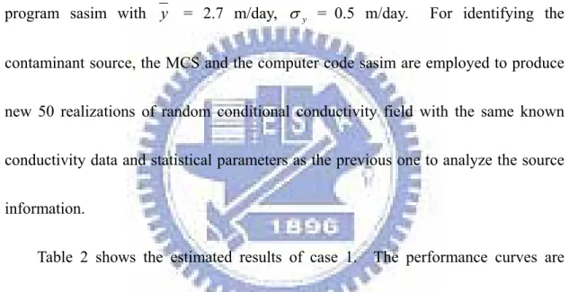
MODFLOW-GWT with the assumed release concentration at known source. Thus, six sampling points H2, J1, M2, N4, P1, and Q3 are taken to identify the source information in the first case study. The hydraulic conductivities and measured concentrations at these sampling points are listed in Table 1. The name of the sampling points given in Table 1 consists of the well name and layer number. Based on the information of the six sampling points, a hypothetical site is generated by the program sasim with y = 2.7 m/day, σy = 0.5 m/day. For identifying the contaminant source, the MCS and the computer code sasim are employed to produce new 50 realizations of random conditional conductivity field with the same known conductivity data and statistical parameters as the previous one to analyze the source information.
Table 2 shows the estimated results of case 1. The performance curves are shown in Fig. 5 in which the horizontal and vertical axes present the MCS runs and the probability of obtaining correct solution, respectively. In Table 2, the results indicate that in identifying the source location from 36 candidate sources, the use of six sampling points gives a 50 % chance to obtain the correct result. It implies that among those 50 MCS runs, a total of 25 runs obtain the correct source location (220 m, 540 m, -9 m). Such a result is very promising if compared with the chance of 2.8 % that is to randomly select one out of 36 candidate sources from a heterogeneous
aquifer formation. Besides, base the guideline of well design, when three sampling points C1, D2, and E2 are added to identify the source location, the average identification probability of the real source increases to 54 %. Moreover, when the sampling points I1, K2, and O2 are added to identify the source location, the chance can be increased to 56 % and more likely to estimate the source location. Thus, if the aquifer is heterogeneous with σy = 0.5, the use of SATS-GWT with6, 9, and 12 sampling points can determine the real source location when employing with the MCS.
The second case assumes that the mean of hydraulic conductivities at the sampling points are also 2.7 m/day, but field conductivity σy = 1.0. Table 3 shows the estimated results when the sampling numbers are 6, 9 and 12, and the performance curves is demonstrated in Fig. 6. The sampling points used to identify the suspicious source location are the same as case 1. When the sampling numbers are six, Table 3 shows that the estimated average probability of correct source location is 18 %, but 40 % chance in getting the wrong location (260m, 540m, -9m). It implies that six sampling points are not enough to obtain the correct result in this case.
As sampling numbers increase to nine, the chance of getting the correct source location increases to 32 %. In contrast, the highest average probability of getting the wrong location (220m, 540m, -15m) is only 20 %. It implies that the use of nine
sampling points can improve the poor estimation of using only six sampling points. Moreover, when sampling numbers increase to 12, the chance of getting the correct source location is increased to 40 %. Contrarily, the highest average probability of obtaining the wrong location (260m, 540m, -9m) is 22 %. The chance of getting the correct source location is higher than those of other suspicious locations. Thus, if the aquifer is heterogeneous with σy = 1.0, the use of 9 or 12 sampling points can both give good source location estimation from statistical viewpoint.
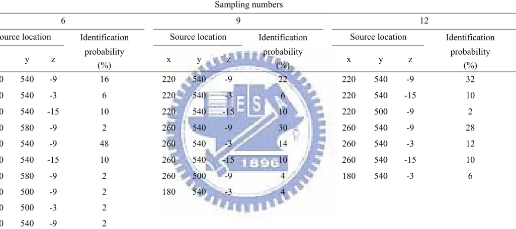
The third case considers σy = 1.5; the aquifer has more variety in hydraulic conductivity. Fig. 7 shows that the chance of obtaining the correct source location is 16 % for six sampling points after 50 MCS runs, and the chance is 22 % after 50 MCS runs for nine sampling points. However, the highest chance of getting the wrong location (260m, 540m, -9m) is 48 % for six sampling points, and the highest chance of getting the wrong location (260m, 540m, -9m) is 30 % for nine sampling points. Thus, the estimated results of using six and nine sampling points are both poor as indicated in Table 4. When sampling numbers increase to 12, the chance of getting the correct source location is increased to 32 %. The highest average probability of finding the wrong location (260m, 540m, -9m) decreases to 28 %. Obviously, the increase of sampling points improves the estimated result. It also implies that the contaminant source in a highly heterogeneous aquifer is difficult to identify and more
sampling points can have higher chance to get the correct source location estimation. In sum, the performance of source identification becomes poorer as the standard deviation of the field hydraulic conductivity increases. However, the influence of the degree of uncertainty in hydraulic conductivity on the estimated result can be improved by increasing the number of sampling points as demonstrated in the analysis of cases 2 and 3.
3.3 Scenario 2: Application of the LHS Method
In order to evaluate whether 50 MCS runs is sufficient or not to represent the source identification results in heterogeneous aquifers, 1000 simulations runs are considered for a chosen σy. However, 1000 simulation runs may require a large number of simulation times. Note that SATS-GWT takes about 7 hours to obtain the solution for each case when performed on a personal computer with 2.4 G Pentium IV
CPU and 256 MB RAM. Thus, the LHS method is applied to save simulation times and ensure that all portions of conductivity field are sampled. To calculate the results of LHS method, the effect of standard deviation of the hydraulic conductivity and the number of sampling points on source identification probability are investigated again in the following case studies.
First, the program sasim is employed to produce M = 1000 random conductivity
previous cases in scenario 1. Figures 8 shows three cumulative probability distributions of the generated 1000 conductivity fields for the cases of σy = 0.5, 1.0, and 1.5 m/day. For σy = 0.5 case, the standard deviation of each lnK field varies
from 0.4791 to 0.5218 and has an average of 0.4997. For σy = 1.0 case, the standard deviation of each lnK field varies from 0. 9496 to 1.0367 and has an average
of 0.9901. However, for the case of σy = 1.5, the σy appears to vary from 1.4089 to 1.6037 with an average of 1.4878. The results indicate that the range of
y
σ for 1000 conductivity fields is increased with larger σy.
To obtain the LHS samples in this study, M is chosen as 1000 and N is chosen
as 50. In other words, totally 50 conductivity fields are selected from 1000 conditioning conductivity fields by LHS for the identification of the source location using the model SATS-GWT.
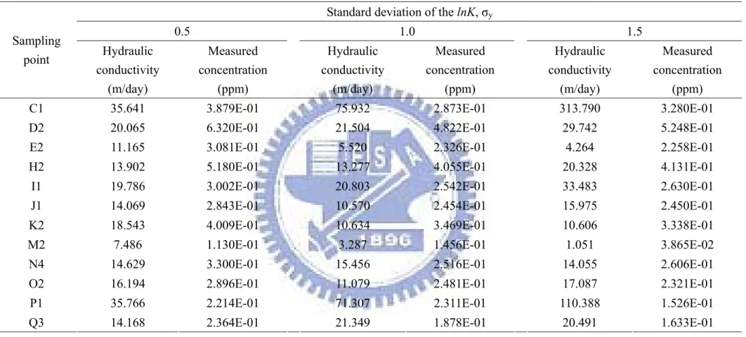
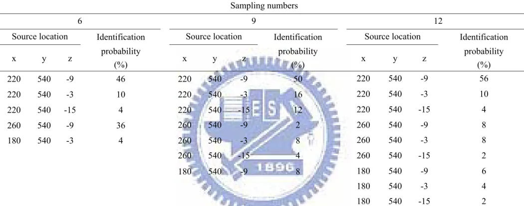
Table 5 shows the hydraulic conductivities and measured concentrations at the sampling points in this scenario. Tables 6, 7, and 8 show the estimated results for cases 4, 5, and 6, respectively. In case 4, the estimate results are listed in Table 6 and the performance curves are shown in Fig. 9. The chance of getting the correct source location (220m, 540m, -9m) with six sampling points is 46 % after 50 LHS runs. It is higher than those of other locations. Besides, when the sampling points are increased to 9 and 12, the chance of getting the correct source location are also
increased to 50 % and 52 %, respectively. These estimated results are similar to those of case 1.
The estimated results for case 5 is given in Table 7 and the performance curves can be seen in Fig. 10. When sampling numbers are six, the chance of getting the correct source location is only 20 %, but the highest chance of getting the wrong location (260m, 540m, -9m) is also 20 %. This result implies that the chance for obtaining the correct source location is not high. However, when sampling numbers increases to nine, the chance of getting the correct source location is increased to 26 % and the highest chance of getting the wrong location (260m, 540m, -9m) is 24 %. It implies that the poor result with only six sampling points can be improved as the sampling points are increased to nine. Moreover, the chance of getting correct source location increases to 28 % when sampling numbers are 12 and the highest chance of getting the wrong location (220m, 540m, -3m) decreases to 18 %. Thus, the result shows that at least nine sampling points are needed to ensure better source location estimation in this case in a statistical sense.
The case 6 considers σy being equal to 1.5. In Table 8, when sampling numbers are six and nine, the chances of getting the correct source location are 16 % and 20 %, respectively. The highest chance of getting the wrong location (260m, 540m, -9m) is 30 % for six sampling points, and the highest chance of getting the
wrong location (260m, 540m, -9m) is 20 % for nine sampling points. Both results in estimating the chance of correct source location are lower than the highest chance of getting a wrong location. However, when sampling numbers increase to 12, the results indicate that the identification probability increases to 24 % and the highest chance of getting the wrong location (260m, 540m, -9m) is 18 %. It implies that the chance of obtaining correct source location with 12 sampling numbers can improve poor estimated results with the six or nine sampling points. Figure 11 shows that the performance curves for sampling points 6, 9, and 12 and indicate that the result of 12 sampling points is generally higher than the results of sampling numbers 6 and 9 after 50 LHS runs.
Thus, both MCS and LHS method obtain similar estimated results in getting correct source information when employing the SATS-GWT with 6, 9, and 12 sampling points for aquifer with conditioning random conductivity field with σy = 0.5, 1.0 and 1.5 m/day.
3.4 Scenario 3: Effect of Sampling Point Patterns
In scenario 1, six sampling points with four concentration zones are used to identify the real source location. This scenario compares the effect of the pattern of sampling location on source identification probability in four cases for heterogeneous
aquifers with σy = 0.5 m/day. The hydraulic conductivities and measured concentrations at the sampling points are shown in Table 9.
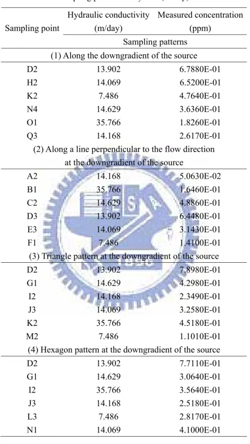
In case 1, the sampling points D2, H2, K2, N4, O1, and Q3 are assumed to install from x = 300 m to x = 500 m with a uniform interval of 40 m along the x-axis. The
identification results are shown in Table 10. When the sampling points are taken along the downgradient of the source, the average identification probability of the correct source is 20 %. The highest chance of getting the wrong location (220m, 540m, -3m) is 30 %. Thus, this sampling location pattern is not suitable for estimating the correct source location. In case 2, the sampling points A2, B1, C2, D3, E3, and F1 are assumed to install from y = 420 m to y = 620 m with a uniform interval of 40 m along the y-axis. The results indicate that the average identification probability of the real source location is only 8 %, but the highest chance of getting the wrong location (180m, 540m, -3m) is 46 %. It implies that when the sampling points are taken along a line perpendicular to the flow direction at the downgradient of the source. The result of estimating the real source location is also poor.
In case 3, when the sampling points D2, G1, I2, J3, K2, and M2 are arranged in a triangle pattern at the downgradient of the source. The average identification probability of the real source location is increased to 22 %, but the highest chance of the wrong location (220m, 540m, -3m) is 28 %. It still can not get better source
location estimation result. In case 4, the sampling points D2, G1, I2, J3, L3, and N1 are installed in a hexagon pattern at the downgradient of the source. The chance of getting the correct source location is increased to 50 %. The highest chance of getting the wrong location (180m, 540m, -9m) is decreased to 12 %. It implies such an arrangement of the sampling points can effectively identify the correct source.
The performance curves for each case are shown in Fig. 12. When the sampling points are in a hexagon pattern at the downgradient of the source, the average identification probabilities curve are generally higher than other patterns in cases 1 to case 3. The chance is also similar with the sampling location pattern taken from four concentration zones. Thus, for getting good identification result in the heterogeneous aquifer with σy = 0.5, we suggest allocating the sampling points in a hexagon pattern at the downgradient of the source if the information of four concentration zones is not available.
CHAPTER 4 Conclusions
This study investigates the problem of promoting the probability for finding a groundwater contamination source in three-dimensional heterogeneous aquifers. Different heterogeneous aquifers are considered when employing the computer model SATS-GWT to estimate source location. The random hydraulic conductivity fields, generated by the program sasim with known conductivity as conditioning data, are log-normally distributed with a given mean, standard deviation of lnK, and spatial
correlation structure. Three scenarios are designed to study the effects of various numbers and patterns of sampling points on the probability of obtaining correct source location.
In the first scenario, as the standard deviation of the hydraulic conductivity increases, the results of source identification get poorer. The results of MCS show that the use of six sampling points can give up to 50 % chance to get the correct source location for σy = 0.5. However, as the σy is increased to 1.0, nine sampling points is needed to get more chance of finding correct source location. Moreover, when the σy is increased to 1.5, 12 sampling points is needed.
In the second scenario, LHS is applied as an alternative to the MCS along with a source identification model for estimating the source location in three-dimensional
heterogeneous aquifers. A total of 1000 heterogeneous aquifers which have the same conditioning data and statistical parameters as scenario 1 are generated by the program sasim again. Those conductivity fields are sampled by LHS method and used to identify the source location by the model SATS-GWT again. The result demonstrates that when the σy = 0.5, 1.0 and 1.5, the chance to obtain correct source location are all similar to MCS result from the statistical viewpoint.
The third scenario is to compare the effect of the five sampling point patterns on source identification estimation. The result demonstrates that when σy = 0.5, the sampling points are arranged in a hexagon pattern at the downgradient of the source will also have good chance to get correct source location.
In sum, this study investigates different degrees of aquifer heterogeneity and different sampling techniques on the probability of identifying a contaminant source. It can be concluded that the probability of identifying a contaminant source location and the effect of the uncertainty in heterogeneous groundwater sites can be reduced as the sampling numbers are increased. In addition, we suggest the sampling points allocated in a hexagon pattern at the downgradient of the source can obtain better identification results if the sampling points with four concentration zones are not available.
References
Bagtzoglou, A. C., D. E. Dougherty, and A. F. B. Tompson (1992), Applications of particle methods to reliable identification of groundwater pollution sources,
Water Resour Mgmt. 6:15-23.
Chang, T. H., and H. D. Yeh (2005), Combining tabu search and simulated annealing for identifying three-dimensional groundwater contaminant source, M. S. thesis,
NCTU.
Deutsch, C. V., and A. G. Journel (1998), GSLIB: Geostatistical Software Library and User’s Guide, 2nd ed, 369 pp., Oxford Univ. Press, New York.
Gwo, J. P., L. E. Toran, M. D. Morris, and G. V. Wilson (1996), Subsurface stormflow modeling with sensitivity using a latin-hypercube sampling technique, Ground Water, 34(5), 811-818.
Harbaugh, A. W., E. R. Banta, M. C. Hill, and M. G. McDonald (2000), MODFLOW-2000, The U.S. Geological survey modular ground-water model-user guide to modularization concepts and the ground-water process,
Open File, 00-92, 121 pp., U.S. Geological Survey, Reston, VA.
IMSL (2003), Fortran Library User’s Guide Stat/Library, Volume 2 of 2, Visual
Konikow, L. F., D. J. Goode, and G. Z. Hornberger (1996), A three-dimensional method of characteristics solute-transport model (MOC3D), U.S. Geological Survey Water-Resources Investigations Report 96-4267.
Mahar P. S., and B. Datta (1997), Optimal monitoring network and ground-water pollution source identification, J. Water Res. Plng. and Mgmt. ASCE, 123 (4),
199-207.
Meyer, P. D, and E. D. B, Jr (1988), A method for locating wells in a groundwater monitoring network under conditions of uncertainty, Water Resour. Res., 24(8),
1277-1282.
Meyer, P. D, A. J. Valocchi, and J. W. Eheart (1994), Monitoring network design to provide initial detection of groundwater contamination, Water Resour. Res.,
30(9), 2647-2659.
Mckay, M.D., W.J. Conover, and R.J. Beckman (1979), A comparison of three methods for electing values of input variables in the analysis of output from a computer code, Technometrics, 21, 239-245.
Storck, P., J. W. Eheart, and A. J. Valocchi (1997), A method for the optimal location of monitoring wells for detection of groundwater contamination in three-dimensional heterogeneous aquifers, Water Resour. Res. 33(9), 2081-2088.
correlated random hydraulic conductivity fields, Water Resour. Res., 39 (8),
1226.
Zheng, C., and G.D. Bennett (1995), Applied contaminant transport modeling: Theory and practice. Van Nostrand Reinhold, New York, 440 pp.
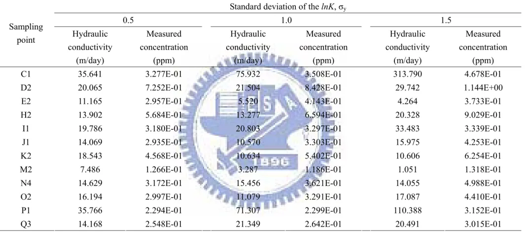
Table 1 The measured concentrations and hydraulic conductivities in monitoring wells for MCS method Standard deviation of the lnK, σy
0.5 1.0 1.5 Sampling point Hydraulic conductivity (m/day) Measured concentration (ppm) Hydraulic conductivity (m/day) Measured concentration (ppm) Hydraulic conductivity (m/day) Measured concentration (ppm)
C1 35.641 3.277E-01 75.932 3.508E-01 313.790 4.678E-01 D2 20.065 7.252E-01 21.504 8.428E-01 29.742 1.144E+00 E2 11.165 2.957E-01 5.520 4.143E-01 4.264 3.733E-01 H2 13.902 5.684E-01 13.277 6.594E-01 20.328 9.029E-01
I1 19.786 3.180E-01 20.803 3.297E-01 33.483 3.339E-01 J1 14.069 2.935E-01 10.570 3.303E-01 15.975 4.253E-01 K2 18.543 4.568E-01 10.634 5.402E-01 10.606 6.254E-01 M2 7.486 1.266E-01 3.287 1.186E-01 1.051 1.318E-01
N4 14.629 3.172E-01 15.456 3.621E-01 14.055 4.988E-01 O2 16.194 2.997E-01 11.079 3.291E-01 17.087 4.410E-01 P1 35.766 2.294E-01 71.307 2.299E-01 110.388 3.152E-01 Q3 14.168 2.548E-01 21.349 2.642E-01 20.491 3.015E-01
Table 2 Results of source identification for MCS method as σy = 0.5 (m/day)
Sampling numbers
6 9 12 Source location Source location Source location
x y z Identification probability (%) x y z Identification probability (%) x y z Identification probability (%) 220 540 -9 50 220 540 -9 54 220 540 -9 56 220 540 -3 20 220 540 -3 10 220 540 -3 18 260 540 -9 22 260 540 -9 12 220 540 -15 4 260 540 -3 4 260 540 -3 22 260 540 -9 6 180 540 -9 4 180 540 -3 2 260 540 -3 12 180 540 -3 4
Table 3 Results of source identification for MCS method as σy = 1.0 (m/day)
Sampling numbers
6 9 12 Source location Source location Source location
x y z Identification probability (%) x y z Identification probability (%) x y z Identification probability (%) 220 540 -9 18 220 540 -9 32 220 540 -9 40 220 540 -3 10 220 540 -3 6 220 540 -3 6 220 540 -15 6 220 540 -15 20 220 540 -15 8 220 500 -9 2 260 540 -9 16 260 540 -9 22 260 540 -9 40 260 540 -3 8 260 540 -3 4 260 540 -3 4 260 540 -15 6 260 540 -15 12 260 540 -15 10 260 580 -9 2 180 540 -9 4 260 500 -9 2 180 540 -9 4 180 540 -3 2 260 500 -3 2 180 540 -3 6 180 500 -15 2 180 540 -9 4 180 540 -3 2
Table 4Results of source identification for MCS method as σy = 1.5 (m/day)
Sampling numbers
6 9 12 Source location Source location Source location
x y z Identification probability (%) x y z Identification probability (%) x y z Identification probability (%) 220 540 -9 16 220 540 -9 22 220 540 -9 32 220 540 -3 6 220 540 -3 6 220 540 -15 10 220 540 -15 10 220 540 -15 10 220 500 -9 2 220 580 -9 2 260 540 -9 30 260 540 -9 28 260 540 -9 48 260 540 -3 14 260 540 -3 12 260 540 -15 10 260 540 -15 10 260 540 -15 10 260 580 -9 2 260 500 -9 4 180 540 -3 6 260 500 -9 2 180 540 -3 4 260 500 -3 2 180 540 -9 2
Table 5 The measured concentrations and hydraulic conductivities in monitoring wells for LHS method Standard deviation of the lnK, σy
0.5 1.0 1.5 Sampling point Hydraulic conductivity (m/day) Measured concentration (ppm) Hydraulic conductivity (m/day) Measured concentration (ppm) Hydraulic conductivity (m/day) Measured concentration (ppm)
C1 35.641 3.879E-01 75.932 2.873E-01 313.790 3.280E-01 D2 20.065 6.320E-01 21.504 4.822E-01 29.742 5.248E-01 E2 11.165 3.081E-01 5.520 2.326E-01 4.264 2.258E-01 H2 13.902 5.180E-01 13.277 4.055E-01 20.328 4.131E-01
I1 19.786 3.002E-01 20.803 2.542E-01 33.483 2.630E-01 J1 14.069 2.843E-01 10.570 2.454E-01 15.975 2.450E-01 K2 18.543 4.009E-01 10.634 3.469E-01 10.606 3.338E-01 M2 7.486 1.130E-01 3.287 1.456E-01 1.051 3.865E-02
N4 14.629 3.300E-01 15.456 2.516E-01 14.055 2.606E-01 O2 16.194 2.896E-01 11.079 2.481E-01 17.087 2.321E-01 P1 35.766 2.214E-01 71.307 2.311E-01 110.388 1.526E-01 Q3 14.168 2.364E-01 21.349 1.878E-01 20.491 1.633E-01
Table 6 Results of source identification for LHS method as σy = 0.5 (m/day)
Sampling numbers
6 9 12 Source location Source location Source location
x y z Identification probability (%) x y z Identification probability (%) x y z Identification probability (%) 220 540 -9 46 220 540 -9 50 220 540 -9 56 220 540 -3 10 220 540 -3 16 220 540 -3 10 220 540 -15 4 220 540 -15 12 220 540 -15 4 260 540 -9 36 260 540 -9 2 260 540 -9 8 180 540 -3 4 260 540 -3 8 260 540 -3 8 260 540 -15 4 260 540 -15 2 180 540 -9 8 180 540 -9 6 180 540 -3 4 180 540 -15 2 Note that the real source is located at (220m, 540m, -9m), real release concentration is 100 ppm, real release period is 3 years.
Table 7 Results of source identification for LHS method as σy = 1.0 (m/day)
Sampling numbers
6 9 12 Source location Source location Source location
x y z Identification probability (%) x y z Identification probability (%) x y z Identification probability (%) 220 540 -9 20 220 540 -9 26 220 540 -9 28 220 540 -15 10 220 540 -3 12 220 540 -3 18 220 580 -3 2 220 540 -15 2 220 540 -15 2 220 580 -15 2 220 540 -21 2 260 540 -9 6 220 500 -3 2 260 540 -9 24 260 540 -3 12 260 540 -9 20 260 540 -3 18 260 540 -15 2 260 540 -3 6 260 540 -15 6 180 540 -9 10 260 540 -15 8 180 540 -9 8 180 540 -3 12 180 540 -9 14 180 540 -15 2 180 540 -15 6 180 540 -3 6 180 580 -9 2 180 540 -15 6 180 500 -21 2 180 580 -15 4
Table 8 Results of source identification for LHS method as σy = 1.5 (m/day)
Sampling numbers
6 9 12 Source location Source location Source location
x y z Identification Probability (%) x y z Identification Probability (%) x y z Identification Probability (%) 220 540 -9 16 220 540 -9 20 220 540 -9 24 220 540 -3 20 220 540 -3 16 220 540 -3 14 260 540 -9 30 260 540 -9 20 220 540 -15 8 260 540 -3 16 260 540 -3 12 220 500 -15 4 260 580 -9 4 260 580 -3 2 260 540 -9 18 260 500 -9 2 260 500 -15 2 260 540 -3 6 180 540 -9 8 180 540 -9 16 260 540 -15 4 180 540 -3 2 180 540 -3 4 180 540 -9 2 180 580 -9 2 180 540 -15 6 180 540 -3 4 180 580 -9 2 180 540 -15 12 180 500 -15 2 180 500 -21 2
Table 9 The measured concentrations and hydraulic conductivities in different sampling patterns as σy =0.5 (m/day)
Hydraulic conductivity (m/day) Measured concentration (ppm) Sampling point Sampling patterns (1) Along the downgradient of the source
D2 13.902 6.7880E-01 H2 14.069 6.5200E-01 K2 7.486 4.7640E-01 N4 14.629 3.6360E-01 O1 35.766 1.8260E-01 Q3 14.168 2.6170E-01
(2) Along a line perpendicular to the flow direction at the downgradient of the source
A2 14.168 5.0630E-02 B1 35.766 1.6460E-01 C2 14.629 4.8860E-01 D3 13.902 6.4480E-01 E3 14.069 3.1430E-01 F1 7.486 1.4100E-01
(3) Triangle pattern at the downgradient of the source
D2 13.902 7.8980E-01 G1 14.629 4.2980E-01 I2 14.168 2.3490E-01 J3 14.069 3.2580E-01 K2 35.766 4.5180E-01 M2 7.486 1.1010E-01
(4) Hexagon pattern at the downgradient of the source
D2 13.902 7.7110E-01 G1 14.629 3.0640E-01 I2 35.766 3.5640E-01 J3 14.168 2.5180E-01 L3 7.486 2.8170E-01 N1 14.069 4.1000E-01
Table 10 Results of source identification versus sampling location patterns as σy = 0.5 (m/day)
Sampling patterns Along the downgradient of
the source
Along a line perpendicular to the flow direction at the downgradient
of the source
Triangle pattern at the downgradient of the source
Hexagon pattern at the downgradient of the source
Source location
Source location Source location Source location
x y z Identification probability (%) x y z Identification probability (%) x y z Identification probability (%) x y z Identification probability (%) 220 540 -9 20 220 540 -9 8 220 540 -9 22 220 540 -9 50 220 540 -3 30 220 540 -3 28 220 540 -3 28 220 540 -3 8 260 540 -3 8 260 540 -9 2 260 540 -9 6 220 500 -15 2 260 580 -9 2 260 540 -3 2 260 540 -3 8 260 540 -9 10 180 540 -9 16 180 540 -9 14 180 540 -9 12 260 540 -3 8 180 540 -3 22 180 540 -3 46 180 540 -3 20 260 540 -15 6 180 500 -9 2 180 500 -3 2 180 540 -9 12 180 500 -15 2 180 540 -3 4 Note that the real source is located at (220m, 540m, -9m), real release concentration is 100 ppm, real release period is 3 years.
Fig. 1. Flowchart of SATS-GWT. The OFVCALO represent the objective
C onstant head and groundw ater table is located at -5 m
N o flow boundary (0,0,0)
Suspicious zone 24m
C onstant head and groundw ater table is located at 0 m N o flow boundary 40m 1000 m 1000 m X Y Z 220 m A J B Q C G D H E I F M O L N K P 540m 9m S1 40m 6 m
Fig. 4. The aquifer system with an area of 1000m by 1000m and the locations of real source S1, eight suspicious sources near S1, and sampling points A to Q
0 10 20 30 40 50
Number of Monte Carlo Runs
0 0.1 0.2 0.3 0.4 0.5 0.6 0.7 0.8 0.9 1 Probability MCS Method sampling points = 6 sampling points = 9 sampling points = 12
0 10 20 30 40 50
Number of Monte Carlo Runs
0 0.1 0.2 0.3 0.4 0.5 0.6 0.7 0.8 0.9 1 Proba bi li ty MCS Method sampling points = 6 sampling points = 9 sampling points = 12
0 10 20 30 40 50
Number of Monte Carlo Runs
0 0.1 0.2 0.3 0.4 0.5 0.6 0.7 0.8 0.9 1 Proba bi li ty MCS Method sampling points = 6 sampling points = 9 sampling points = 12
0.4 0.5 0.6 0.7 0.8 0.9 1 1.1 1.2 1.3 1.4 1.5 1.6 Standard deviation of lnk 0 0.2 0.4 0.6 0.8 1 P rob abi lity
assign standard deviation of lnk
0.5 1.0 1.5
Fig. 8. The cumulative frequency distribution of 1000 conductivity fields data of σy = 0.5, 1.0, and 1.5 (m/day)
0 10 20 30 40 50
Number of Monte Carlo runs
0 0.1 0.2 0.3 0.4 0.5 0.6 0.7 0.8 0.9 1 P ro bab ilit y LHS Method sampling points = 6 sampling points = 9 sampling points = 12
0 10 20 30 40 50
Number of Monte Carlo runs
0 0.1 0.2 0.3 0.4 0.5 0.6 0.7 0.8 0.9 1 Pr ob ab ility LHS Method sampling points = 6 sampling points = 9 sampling points = 12
0 10 20 30 40 50
Number of Monte Carlo runs
0 0.1 0.2 0.3 0.4 0.5 0.6 0.7 0.8 0.9 1 Pro bability LHS Method sampling points = 6 sampling points = 9 sampling points = 12
0 10 20 30 40 50
Number of Monte Carlo runs
0 0.1 0.2 0.3 0.4 0.5 0.6 0.7 0.8 0.9 1 Probab il ity Sampling patterns
Along the downgradient of the source
Along a line perpendicular to the flow direction at the downgradient of the source
Triangle pattern at the downgradient of the source Hexagon pattern at the downgradient of the source
Fig. 12. The performance curves of the probability versus sampling location patterns as σ =0.5 (m/day) y