STEP-DRAWDOWN DATA-ANALYSIS

S T E P - D R A W D O W N D A T A ANALYSIS By Hund-Der Yeh1

INTRODUCTION

The total drawdown sw in a pumping well consists of the formation loss and the well loss. The equation of the total drawdown sw may be written as (Todd 1980)

sw = BQ + CQP (1)

where Q = the pumping rate; B = the formation constant; p = a constant and greater than one; and C = the well-loss constant. The formation loss

BQ is due to head loss in the aquifer through which the groundwater flows

towards the pumping well. The well loss CQP is caused by the frictional

loss of flow through the well screen and the flow of the water inside the well bore.

For a steady flow to a well in a confined aquifer, the formation constant can be expressed as

„(*

B = (2) 2TTT

where R = the radius of influence; rw = the radius of the pumping well;

and T = the aquifer transmissivity. The value of C depends on the well radius, well construction, and the condition of the well. Based on field ex-perience, Walton (1962) suggested a relationship between the loss constant, C, and the well condition. Since the flow through the well screen and inside the well will usually be turbulent, the well loss is proportional to apth power of the pumping rate, as shown in Eq. 1. Jacob (1946) used a value that p

= 2, while Rorabaugh (1953) concluded that values of p are consistently in

the range near 2.5. In a number of field cases, Lennox (1966) pointed out that the value of p may range as high as 3.5.

EARLIER WORKS FOR ESTIMATING LOSS CONSTANTS

For p = 2, the specific drawdown equation can be obtained from Eq. 1 as

sw

— = B + CQ • (3)

'Assoc. Prof., Dept. of Civ. Engrg., Nat. Chiao Tung Univ., Hsinchu, Taiwan, Republic of China.

Note. Discussion open until March 1, 1990. To extend the closing date one month, a written request must be filed with the ASCE Manager of Journals. The manuscript for this paper was submitted for review and possible publication on May 16, 1988. This paper is part of the Journal of Hydraulic Engineering, Vol. 115, No. 10, October, 1989. ©ASCE, ISSN 0733-9429/89/0010-1426/$1.00 + $.15 per page. Paper No. 23938.

1426

The values of B and C may be determined by plotting sw/Q versus Q and fitting a straight line through the data points (Todd 1980). A linear regression approach was suggested by Nahm (1980) to estimate B and C using Eq. 3.

Rorabaugh (1953) rewrote Eq. 1 as

log (~ - BJ = log C + (p ~ 1) log Q (4) Then a straight line with slope (p — 1) and intercept C will be shown in a

logarithmic plot of {sw/Q — B) versus Q. By assuming different values of

B, a plot of sw/Q — B versus Q on logarithmic paper will be repeated until

a straight line is reached. Then values of p and C can be obtained from the slope and the intercept of the fitted straight line, respectively. This is es-sentially a graphic trial-and-error procedure. Sheahan (1971) developed a method for direct analysis of step-drawdown data using type curves. Both Rorabaugh's method and Sheahan's method are graphic approaches. Rora-baugh's method is more accurate but more time consuming, whereas Shea-han's method is quicker but slightly less accurate (Labadie and Helweg 1975).

A computer code was developed for the step-drawdown test analysis by Labadie and Helweg (1975) using optimization techniques. The best value of p is found by a standard Fibonacci search approach, then the values of

B and C are obtained by solving two simultaneous linear equations.

PRESENT METHOD

The purpose of this paper is to present a method which does not require graphic procedures to analyze the step-drawdown data. The method is based on a nonlinear least-squares approach and the finite-difference Newton's method to determine the loss constants of the aquifer formation and the pumping well. This method has been successfully used by Yeh (1987) to determine the values of aquifer transmissivity and storage coefficient.

Nonlinear Least-Squares

The nonlinear least-squares approach is commonly used for the curve-fit-ting problems, where one is attempcurve-fit-ting to fit the data (x,-,y,), i = 1, 2, . . . ,

n with a relationship y = f(x) that is nonlinear in x. That approach is used

to find the values of loss constants such that the sum of the squares of dif-ferences between the predicted drawdowns and observed drawdowns at the pumping well is minimized. The sum of the square errors is defined as

n n

2e>=2 (*°t - spf <5)

i = i 1=1

where e, = the prediction error; so, = the observed drawdown at the pumping well; and sp, = BQ, + CQ1 = the predicted drawdown at the pumping well. If 2JLi ef is to be a minimum, the first partial derivatives of 2JL, ef with respect to each loss constant must be zero. Thus

— 2

< = -

2 (*»/ - S

PM> = °

<

>

3

Tp, 2 «? = -2 X (*>< - ^P')fif = ° •* <7)

„ n n

T 2 e? = -2 2 (*>< - *Pi)Cfif In 2, = 0 (8)

Finite-Difference Newton's Method

Eqs. 6-8 are nonlinear in terms of the unknown constants B, C, and p. Suppose that variables xu x2, and x3 represent B, C, and p, respectively;

Eqs. 6-8 may be written as one vector equation:

F(X) = 0 (9) where X = the vector with component (xux2,x3y, and F = the vector with

component (/i,/2,/3).

The Jacobian matrix J of partial derivatives of/ with respect to xh where

i, j = 1, 2, 3, is defined as Oft

J(X) = — (10)

dxj

Suppose that X is the exact solution of Eq. 9, in the neighborhood of X; F can be expanded in Taylor series as

F(X + 8X) = F(X) + J(X)8X + 0(8X2) (11)

With the terms of order 8X2 and higher neglected, a set of linear equations

is obtained as follows

8X = r'(X)F(X + 8X) (12) where J is supposed to be nonsingular (Conte and de Boor 1980). Eq. 12

is a linear system and can be solved for the unknown vector 8X as long as the Jacobian matrix has been evaluated. Then an iterative formula can be formed to solve the system of nonlinear equations of Eqs. 6-8 as

x») = X<*-D _ §x ( 1 3 )

where k = the number of iteration.

Some specified tolerances commonly applied to terminate the iteration are

|8X| < XTOL (14) or

|F[XW]| < FTOL (15)

where the values of XTOL and FTOL are predefined depending on the re-quired accuracy of the solutions.

Those partial derivative terms in Eqs. 10 and 12 can be approximated by a finite-difference formula such as

5/2 f2(Xl + AXUX2,X3) - f2(XuXi,X3)

— = (16) where A*i = a small increment to the variable xx.

1428

TABLE 1. Step-Drawdown Test Data (Todd 1980) Pumping rate (m3/d) (D 500 1,000 2,000 2,500 2,750 Drawdown (m) (2) 1.0 2.6 8.9 14.0 18.6

EXAMPLES AND ANALYSIS

Since there are many approaches to estimate the values of B, C, and p, error criteria such as the standard error of estimate (SEE), the mean error (ME), and the mean absolute error (MAE) are chosen to assess the perfor-mance for different methods. The use of those error criteria has been de-scribed in detail by Yeh (1987).

A pumping drawdown data shown in Table 1 was taken from Todd (1980) for a step-drawdown pumping test. Based on Jacob's suggestion p = 2, the estimated drawdown equation is

sw = 8.0 X 10"4g + 2.0 X 10"622 (17)

determined by fitting a straight line from a plot of sw/Q versus Q. A reasonably good initial guess may be made for the loss constants based on knowledge of the in situ aquifer formation and well condition. The initial guess values for analyzing Todd's step-drawdown data are made as follows: 1.0 X 10~4 and 1.0 for B, 1.0 X 10~4 and 10 for C, and 2.0 and 3.0 for p. By choosing 1.0 X 10~4 for XTOL and FTOL, the proposed method using

the iterative formula, Eqs. 12, 13, and 16 for the system of nonlinear equa-tions (Eqs. 6-8) converges to a result of

sw = 2.158 X 10"3e + 4.811 x 10_11G3"318 (18)

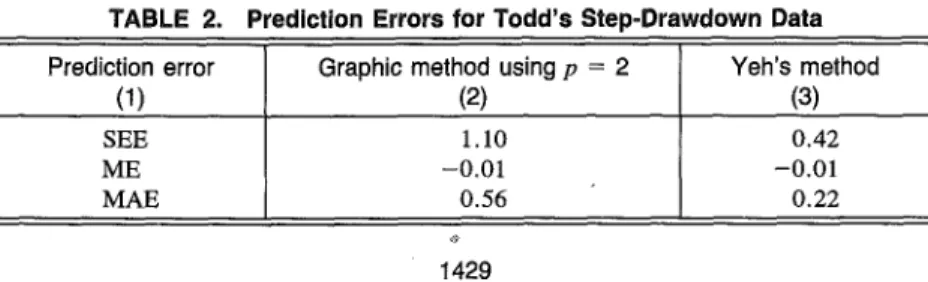
It takes no more than 10 iterations and less than 0.13 central-processing-unit (CPU) sec on a CDC-Cyber 170-720 computer at National Chiao Tung University to obtain this result by the proposed method. Prediction errors by the graphic method using p = 2 and the proposed method are given in Table 2. Obviously, the proposed method yields less prediction errors and better fits Todd's step-drawdown data than the graphic method using p = 2. The estimated formation losses and well losses by the graphic method using Eq. 17 and the proposed method using Eq. 18 are given in Table 3. For for-mation losses the predicted values by Eq. 17 are less than half of the values

TABLE 2. Prediction Errors for Todd's Step-Drawdown Data

Prediction error (1) SEE ME MAE

Graphic method using p = 2 (2) 1.10 -0.01 0.56 Yeh's method (3) 0.42 -0.01 0.22

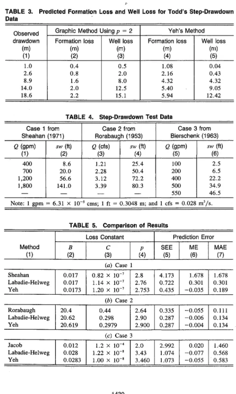
TABLE 3. Predicted Formation Loss and Well Loss for Todd's Step-Drawdown Data Observed drawdown (m) (D 1.0 2.6 8.9 14.0 18.6

Graphic Method Using p = 2 Formation loss (m) (2) 0.4 0.8 1.6 2.0 2.2 Well loss (m) (3) 0.5 2.0 8.0 12.5 15.1 Yeh's Method Formation loss (m) (4) 1.08 2.16 4.32 5.40 5.94 Well loss (m) (5) 0.04 0.43 4.32 9.05 12.42

TABLE 4. Step-Drawdown Test Data Case 1 from Sheahan (1971) Q (gpm) (1) 400 700 1,200 1,800 — sw (ft) (2) 8.6 20.0 56.6 141.0 — Case 2 from Borabaugh (1953) Q (cfs) (3) 1.21 2.28 3.12 3.39 — sw (ft) (4) 25.4 50.4 72.2 80.3 — Case 3 from Bierschenk (1963) Q (9Pm) (5) 100 200 400 500 550 sw (ft) (6) 2.5 6.5 22.2 34.9 46.5 Note: 1 gpm = 6.31 x 10"5 cms; 1 ft = 0.3048 m; and 1 cfs = 0.028 m3/s.

TABLE 5. Comparison of Results

Method (1) Loss Constant B (2) C (3) P (4) Prediction Error SEE (5) ME (6) MAE (7) (a) Case 1 Sheahan Labadie-Helweg Yeh 0.017 0.017 0.0173 0.82 x 10"7 1.14 x 10~7 1.20 x 10"7 2.8 2.76 2.753 4.173 0.722 0.435 1.678 0.301 - 0 . 0 3 5 1.678 0.301 0.189 (b) Case 2 Rorabaugh Labadie-Helweg Yeh 20.4 20.62 20.619 0.44 0.298 0.2979 2.64 2.90 2.900 0.335 0.287 0.287 - 0 . 0 5 5 - 0 . 0 0 6 - 0 . 0 0 4 0.111 0.134 0.134 (c) Case 3 Jacob Labadie-Helweg Yeh 0.012 0.028 0.0283 1.2 x 10~4 1.22 x 10"8 1.00 x 10"8 2.0 3.43 3.460 2.992 1.074 1.073 0.020 - 0 . 0 7 7 - 0 . 0 5 5 1.460 0.568 0.583 1430

by Eq. 18. On the other hand, the well losses would be overestimated by Eq. 17 for the graphic method using p = 2.

Three sets of step-drawdown data listed in Table 4 were selected from the literature by Labadie and Helweg (1975). A comparison of the results by various solution techniques for analyzing these data is made in Table 5. Although these methods proposed by Labadie and Helweg and the writer give about the same results for the second and the third cases, it is found that prediction error MA = 0.301 is exactly the same as MAE by Labadie and Helweg's method in the first case. It means that the predicted draw-downs at the pumping well are all underestimated by Labadie and Helweg's method in the first case.

CONCLUSIONS AND RECOMMENDATIONS

When the Todd's step-drawdown data are analyzed, the predicted for-mation loss values by the graphic method using p = 2 are less than half of the values by the proposed method as shown in Table 3. The ratio for the value of formation constant B in Eqs. 18 and 17 is 2.7. Consequently, based on Eq. 2, the aquifer transmissivity T estimated from the graphic method using p = 2 will be 2.7 times the value of T estimated from the proposed method. For better fit of the observed step-drawdown data and good esti-mation of loss constants, Eq. 1 should be used.

In Eq. 1 a large value of p will give a significantly large value for the well loss. Labadie and Helweg concluded the importance for accurate value of p if the step-drawdown test is to be used to predict drawdown beyond pumping test discharge. Judging from the prediction errors shown in Table 5, it is fair to conclude that the value of p needs be carried out to three decimal places for better accuracy.

A method using nonlinear least-squares and finite-difference Newton's method is proposed to analyze the step-drawdown data. The values of SEE and ME in Tables 2 and 5 examined, the proposed method produces the least statistical errors for the predicted drawdowns at the pumping well. The proposed method has the advantages of quick convergence and high accuracy with the initial guesses of formation constant and well loss constants over a reasonable range.

APPENDIX. REFERENCES

Bierschenk, W. H. (1963). "Determining well efficiency by multiple step-drawdown tests." Publication No. 64, Int. Assoc, of Sci. Hydrol., Berkeley, Calif., 493-507.

Conte, S. D., and de Boor, C. (1980). Elementary numerical analysis, 3rd ed., McGraw-Hill Book Co., New York, N.Y.

Jacob, C. E. (1946). "Drawdown test to determine effect radius of artesian well."

Proc, ASCE, 72(5).

Labadie, J. W., and Helweg, O. J. (1975). "Step-drawdown test analysis by com-puter." Groundwater, 13(5), 438-444.

Lennox, D. H. (1966). "Analysis and application of step-drawdown test." /. Hydr.

Div., ASCE, 92(6), 24-48.

Nahm, G. Y. (1980). "Estimating transmissivity and well loss constant using mul-titate test data from a pumped well." Ground Water, 18(3), 281-285.

Rorabaugh, M. I. (1953). "Graphical and theoretical analysis of step-drawdown test of artesian well." Proc, ASCE, Hydraulic Division, 79, Dec, 362-1-362-23.

Sheahan, N. T. (1971). "Type-curve solution of step-drawdown test. "Ground Water, 9(1), 25-29.

Todd, D. K. (1980). Groundwater hydrology. 2nd ed., John Wiley and Sons, New York, N.Y.

Walton, W. C. (1962). "Selected analytical methods for well and aquifer evalua-tion." Bulletin No. 49, Illinois State Water Survey, Urbana, 111.

Yeh, H. D. (1987). "Theis' solution by nonlinear least-squares and finite-difference Newton's method." Ground Water, 25(6), 710-715.

1432