SHIFTED-JACOBI SERIES ANALYSIS OF LINEAR OPTIMAL-CONTROL SYSTEMS INCORPORATING OBSERVERS

(1)

Shifted-Jacobi

Series Analysis of Linear

Optimal Control Systems Incorporating

0 bseruers

by TSU-TIAN LEE, SHUH-CHUAN TSAY

Institute of Control Engineering, National Chiao Tung University, Hsinchu, 300 Taiwan, Republic of China

and ING-RONG HORNG

Institute of Mechanical Engineering, National Sun Yat-Sen University, Kaohsiung, Taiwan, Republic of China

ABSTRACT : This paper uses the Jacobi series to analyze linear optimal control systems incorporating observers. The method simplijies the system of equations into the successive solution of a set of linear algebraic equations. An illustrative example is included to demonstrate that only a small number (m = 6) of shifted-Jacobi series are needed to obtain an accurate solution.

1. Zntroduction

Orthogonal functions, often used to represent an arbitrary time function, have recently been used to solve control problems. Typical examples are the Walsh functions (l), block-pulse functions (2), Laguerre polynomials (3), Legendre polynomials (4) and Chebyshev series (5).

Stavroulakis and Tzafestas (6) first used the Walsh function to analyze an optimal control system incorporating an observer, but the results were derived based on very unrealistic assumptions. These assumptions were corrected by Kawaji and Tada (7), where the Walsh series was adopted to solve the optimal control law of linear systems incorporating observers. More recently, Chou and Horng (5) applied the shifted-Chebyshev series to approach the same problem.

In the present paper, the shifted-Jacobi series (8) is taken to facilitate research on the analysis of linear optimal control systems incorporating an observer.

ZZ. Problem Statement

Consider a linear time-invariant controllable system s(t) = AX(t) + BU(t) Y(t) = CX(t)

(14

(lb)

(2)

with the performance index

J=

s

m

[Xr(t)QX(t)+Ur(t)RU(t)] dt; Q > 0, R > 0 ₍₂₎

0

where

X(t)

is the

n x

1 state vector, U(t) is the q x 1 control vector,

Y(t)

is the p x 1 output vector, and A, B, C are

n x n, n x q, p x n

constant matrices, respectively.

The problem considered in this paper is to find the optimal control law U*(t) for the system of Eq. (l), and at the same time minimize the performance index (2) subject to the following constraints (9):

(1) an (n-p)-dimensional Luenberger observer is constructed to incorporate the system, and

(2) the optimal control U*(t) is achieved by using digital computation. It is well known that the optimal control law is given by (10)

U*(t) = -R - ‘BrPX(t) = KX(t) where the superscript

T

denotes transpose, and P is the solution of the Riccatti equation :

ArP+PA+Q-PBR-lB=P = 0.

(3)

unique positive-definite

But, in general application, only the output vector

Y(t)

is available for measurement. In this case, the control signal may be realized with (n-p)-dimensional state observers (11)

k(t) = DZ(t) +

GY(t)

+HV(t) (4a)

X(t) = MY(t)+NZ(t) U*(t) = Kg(t) where

Z(t)

is a

(n-p) x

1 vector and D, G, H, M, N dimensions. For the dynamic system of (4) to be relationship must be hold (12):

Z(t) = UX(t) +

e(t)

k(t) =

De(t) where

(4b)

(5)

are matrices of appropriate an observer, the following

(6) (7)

UA-DU = GC _(ga)

H-UB=O _(gb)

MC+NU=I, (8~)

where I, stands for an

n x n

identity matrix. Substituting Eqs (4b), (6) and (8~) into (5), we can obtain

U*(t) = KX(t) + KNe(t). (9)

Inserting Eq. (9) into (1) yields

%(t) = (A + BK)X(t) + BKNe(t) A

&X(t) + Be(t).

(10)

It follows from Eq. (9) that the solution of (7) and (10) is necessary for the

(3)

Shifted-Jacobi Series Analysis

determination of the control law. In the next section, we adopt the shifted-Jacobi

series to carry out the solution of these equations. This approach will result in an

algebraic matrix equation which is conveniently available for digital computation.

ZZZ. Shifted-Jacobi Series Approach

The Jacobi polynomial can be represented in terms of a hypergeometric function

in the interval - 1 < 2 < 1

(11)

In the form, the subscripts 2 and 1 become clear. The leading subscript 2 indicates

that two Pochhammer symbols in the numerator and the final subscript 1 indicates

one Pochhammer symbol in the denominator. We try to transform the independent

variable into values between 0 and tf, and let

t l+Z -_=_

t /

2

.

Then, the shifted-Jacobi polynomials become

where

t,

is the final time and a and

b

are parameters with

a > -

1,

b 3 -

1 and

(a+l)n=(a+l)(a+2)...(a+n)

(a+l), =

1. Letc=a+b+l,then

The recursive formulas for shifted-Jacobi polynomials are

Jo(t) =

1

Jl(t) = -(b+

l)+(c+ 1) ;

0

Jz(t) =+ (b+l),-2(b+2)(c+2) J(t)

J-V’(b+l)

n n. I 1+ t (_l)k(c+n)k t

K

k=l

(b+l),iy

_()I

(13)

291

Vol. 321, No. 5, pp. 289-298, May 1986

(4)

with

2n(n + a + b) (2n + a + b - 2)J,(t)

=(2n+a+b-1) (2n+a+b)(2n+a+b-2) ( 2t,-1 t ) +a -b 2 ‘1

Jn-10)

-2(n+a-1)(n+b-1)(2n+a+b)J,_2(t). (14)

The orthogonality condition is

s

t’

tb(tf -

tyJ,,(t)J,,,(t) dt =

0

nZm (15) n=m

where r(s) stands for the gamma function. Note that an arbitrary time function f(t) can be approximated by the Jacobi polynomials as

f(t) = f.

f,J,(t).

(16)

For practical application, we use only the finite-term of the series to approximate f(t). That is m-l

_I-@)

=

“z.

.LJ&)

=

f'J(t) (17) where

fT =

cfo,

fl~.*.,fm-lI

and

JT =

[Jo@), J1(t), . . . , J,- l(t)l.

The Jacobi coefficient fj is obtained by minimizing the integral square error

Using the necessary condition of minimizing E aE %=O j=O, 1,2 ,..., m-l J we obtain

(18)

(19) (2n + c) (n!)T(n + c) s ff

f” = T(n+a+ l)T(n+b+ l)t(fa+b+l O tb(tJ- t)Y(t)J”(t) dt

n=O, 1,2 ,..., m-l. (20)

292

Journal of the Franklin Institute Pergamon Journals Ltd.

(5)

Shifted-Jacobi Series Analysis The integration for the shifted-Jacobi series can be represented by (8)

s

f

J&7

dt’ = tf

(n+c)

0 (2n+c+ 1)(2n+c) Jn+l@)

(a-4

+ (*n+c+l)(2n+c-1) Jn(t) (n+a)(n+b) -(2n+c)(2n+c-1)(2n+c+ 1) Jn-1(t) (-l)“r(n+b+l) + (n+c- l)(n+ l)!T(b) Jo(t)

1 ’

n = 0, l,...,m-1 (21) or in vector form s f J(t’) dt’ = FJ(t) ₍₂₂₎ 0

where Fis the operational matrix of integration, given by (23) on the next page. Now, we wish to represent the state vector X(t) and error vector e(t) by shifted- Jacobi polynomials :

m-l

e(t) = c &J,(t) = E’J(t)

n=O (24)

m-l

X(t) = c X,J,(t) = XTJ(t)

n=O (25)

where E, and X, are the coefficients of the Jacobi series for e(t) and X(t), respectively. If E, and X, can be determined, the desired control law can be expanded in terms of shifted Jacobi series as:

U*(t) = (KXT + KNET)J(t). ₍₂₆₎

Using these identities

s f k(t’) dt’ = X(t) - x(0) ₍₂₇₎ 0 s f k(t’) dt’ = e(t)-e(0) ₍₂₈₎ 0 we can obtain ET = [e(O), 0,. . . , 0] + DETF ₍₂₉₎ and

XT = [x(o), 0,. . . , 01 + AXTF + BETF. ₍₃₀₎

Vol. 321, No. 5, pp. 289-298, May 1986

(6)

F

=

@A

. . . . . .

r

b+l

I

c+l -(b+l)(a+l)

r(b+2)

-___

c(c+ l)(c+2)

2!cI-(b)

T(b

+

3) (w;~~;) (c +

2)4!r(b)

(-1)m-2f(b+m-l) _(c+ m - 3) (m - l)!T(b) (-l)“-‘=(b+m) _(c+ m - 2) (m)!T(b)

tb+m-2i(a+m-2)

(~+2m-4)(~+2m-5)(i+rn-3) 0 1 c+l

a-b

(c+l)(c+3)

_-(b+2)@+2)

(c+l)(c+3)(c+4) 0 0 0

(a-b)

(c+2m-3)(c+2m-5)

(b+m-l)(a+m-1)

(c+2m-2)(c+2m-3)(c+m-2)

0 c+l (c +,2”;+ 3) (c+3)(c+5)

_-(b+3)@+3)

(c+2)(c+5)@+6) 0 0

(c+m-2)

(c+m-(3)ICb;2m-4)

_{(c+2m-al)o+2m-3)}

(7)

Shifted-Jacobi Series Analysis Equations (29) and (30) can be rewitten as

E = (D @ FT)E + E(0)

X = (A @ FT)X + (fi @ F=)E + (h @I I)X(O) where

E(0) = [e(O), 0,. . . , 01'

(31) (32)

X(0) = [X(O), 0,. . . ) O] = and the operation h @I FT is a Kronecker product (13)

i(t) = -1.52(t)- 1.25Y(t)- U(t), Z(0) = 0.5

m =

(y)

zw+(

1:5)

Y(t)

where U = [ - 1.5, 11. One can identify that

A=A+BK=(_;.5, _;), &BKN=(_;).

The numerical solutions of X and E are shown as follows: (i) whena=0,b=1,m=6andtf=5sec ET = [ -0.0266730, 0.06468 11, - 0.0686554 0.0468477, - 0.0233069, -0.01006241 XT = [ 0.188055, 0.08 1498, -0.179148, +0.051450 0.026011, -0.211355, 0.096915, 0.025337 0.007720, - 0.009478 -0.032898, 0.014465

1 .

Hence the optimal control is

U*(t) = 0.2814205,(t)-0.0244275,(t)-0.2404625,(t) +0.1493765,(t)-0.044626J,(t)+O.O1031J,(t). (ii) When a = 0, b = 1, m = 8 and tf = 5 set

ET = C-0.026548, 0.064379, -0.068371, 0.046578 -0.023388, 0.009301, - 0.003051, 0.000898] XT = 0.1869905, 0.0824952, -0.1792262, 0.0514082

0.0265524, -0.2115233, 0.0967997, 0.0252193

0.0077628, -0.0329158, -0.0087817, 0.0140254, -0.0041601, 0.0030914, -0.0008142 0.0011105

1 -

Vol. 321. No. 5, pp. 28%29X, May 1986

(8)

The optimal control is

U* = 0.280490-0.0234165,(t)-0.240401J,(t) +O.l48910J,(t)-0.0446605&)+0.010154J,(t) -0.0025745&)+0.000787.l,@).

(iii) When a = 0, b = 0, m = 6 and tr = 5 set (i.e. shifted-Legendre series)

ET = [ -0.0999381, 0.2202352, - 0.2060435 +0.1292673, -0.0606371, 0.02526551 XT = [ 0.0767032, 0.3308101, -0.3451541 0.1486299, -0.3061541, 0.8152940 0.0648212, 0.0318698, - 0.0240565 0.1120718, - 0.0866035, + 0.0358856

1 ’

The optimal control is

U* = 0.1637466+0.35029615,(t)-0.64224535,(t)

+0.33857105,(t) - 0.09943585,(t) +0.02506635,(t). The exact solution is

e(t) = 0.75 exp (- 1.5t) and

U*(t) = -0.75 exp (- 1.5t)-0.55 exp (-0.5t) cos (0.5t) + 1.9 exp (-0.5t) sin (0.5t).

As can be seen from Tables I and II, the approximate solutions obtained by the

TABLE I

Numerical solution of e(t)

a = 0, b = 1 a=O,b=l a=b=O t Exact approx. (m = 6) m=8 m=6 0.0 -0.750000 -0.726300 0.1 -0.645531 - 0.633493 0.2 -0.555614 -0.551735 0.3 -0.478221 -0.479311 0.4 -0.411609 -0.415364 0.5 -0.354275 - 0.359094 0.6 -0.304927 -0.309751 0.7 -0.262453 - 0.266637 0.8 -0.225896 - 0.229 106 0.9 -0.194430 -0.196555 1.0 -0.167348 -0.168429 - 0.747995 -0.741487 - 0.644946 -0.643566 -0.555728 -0.557281 -0.478995 -0.481435 -0.411996 -0.415001 -0.354563 -0.357025 -0.305083 -0.306620 -0.262488 -0.262963 -0.225845 -0.225295 -0.194336 -0.192918 - 0.167246 -0.165188 296

Journal of the Franklin Institute Pergamon Journals Ltd.

(9)

Shifted-Jacobi Series Analysis

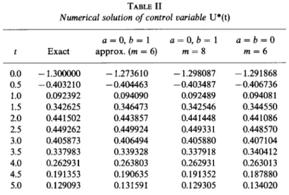
TABLE II

Numerical solution of control variable U*(t)

a=O,b=l a=O,b= 1 a=b=O

t Exact approx. (m = 6) m=8 m=6 0.0 - 1.300000 - 1.273610 - 1.298087 - 1.291868 0.5 -0.403210 - 0.404463 - 0.403487 - 0.406736 1.0 0.092392 0.094090 0.092489 0.09408 1 1.5 0.342625 0.346473 0.342546 0.344550 2.0 0.441502 0.443857 0.441448 0.441086 2.5 0.449262 0.449924 0.449331 0.448570 3.0 0.405873 0.406494 0.405880 0.407104 3.5 0.337983 0.339328 0.337918 0.340412 4.0 0.26293 1 0.263803 0.262931 0.263013 4.5 0.191353 0.190635 0.191352 0.187880 5.0 0.129093 0.131591 0.129305 0.134020

shifted-Jacobi series are very close to the exact solution, even when a small number (m = 6) of shifted-Jacobi polynomials is used.

IV. Conclusions

In this paper, shifted-Jacobi polynomials are adopted to solve optimal control systems incorporating observers. The proposed technique simplifies the system of equations into the successive solution of a set of linear algebraic equations. Thus, the computation is effective and straightforward. Moreover, only a small number of the shifted-Jacobi series (m = 6) are needed to obtain a satisfactory solution, hence it is seen that the method does not, in general, need an excessive capacity of memory and computing time.

References

(1) C. F. Chen and C. H. Hsiao, “A state space approach to Walsh series solution of linear

systems”, Int. J. System Sci., Vol. 6, pp. 833-858, 1975.

(2) N. S. Hsu and B. Cheng, “Analysis and optimal control of time-varying linear systems via block pulse function”, Int. J. Control, Vol. 33, No. 6, pp. 1107-1122, 1981.

(3) C. Hwang and Y. P. Shih, “Laguerre operational matrices for fractional calculus and applications”, Int. J. Control, Vol. 34, pp. 577-584, 1981.

(4) R. Y. Chang and M. L. Wang, “Analysis of stiff system via method of shifted Legendre functions”, Znt. J. System Sci., Vol. 15, No. 6, pp. 627-637, 1984.

(5) J. H. Chou and I.-R. Horng, “Shifted Chebyshev series analysis of linear optimal control systems incorporating observers”, Znt. J. Control, Vol. 41, pp. 129-134,

1985.

(6) P. Stavroulakis and S. Tzafestas, “Walsh series approach to observer with filter design in optimal control system”, Znt. J. Control, Vol. 26, pp. 721-736, 1977.

(7) S. Kawaji and R. Tada, “Walsh series analysis in optimal control systems incorporating observers”, Znt. J. Control, Vol. 37, pp. 455462, 1983.

Vol. 321, No. 5, pp. 289-298, May 1986

(10)

(8) Y. L. Luke, “The Special Functions and Their Approximations”, Academic Press, New York, 1969.

(9) J. J. Bongiorno and D. C. Youla, “On observers in multi-variable control systems”, Int. J.

Control, Vol. 8, pp. 221-243, 1968.

(10) B. D. 0. Anderson and J. B. Moore, “Linear Optimal Control”, Prentice-Hall, Englewood Cliffs, 1971.

(11) D. G. Luenberger, “An introduction to observers”, IEEE Trans. Aut. Control, Vol. AC-

16, No. 6, pp. 596602, 1971.

(12) S. Kawaji, “Block-pulse series analysis of linear systems incorporating observers”, Int. .I.

Control, Vol. 37, pp. 1113-1120, 1983.

(13) P. Lancaster, “Theory of Matrices”, Academic Press, New York, 1969.