利用導場向量空間投影進行腦部獨立活動訊號源之時空造影

(1)

國

立

交

通

大

學

資訊科學與工程研究所

碩

士

論

文

利

用

導

場

向

量

空

間

投

影

進行腦部獨立活動訊號源之時空造影

Lead Field Vector Space Projection for Spatiotemporal

Imaging of Independent Brain Activities

研究生：陳姿樺

指導教授：陳永昇博士

中

中華

華

_{華民}

華

民

_{民國}

民

國

_{國九}

九

_{九十}

_{十七}

十

七

_{七年}

年

_{年八}

年

八

_{八月}

月

_月

(2)

(3)

利用導場向量空間投影進行腦部獨立活動訊號源之時空造影

Lead Field Vector Space Projection for Spatiotemporal Imaging

of Independent Brain Activities

研究生：陳姿樺 Student：Tzu-Hua Chen

指導教授：陳永昇 Advisor：Yong-Sheng Chen

國立交通大學

資訊科學與工程研究所

碩士論文

A Thesis

Submitted to Institute of Computer Science and Engineering College of Computer Science

National Chiao Tung University in partial Fulfillment of the Requirements

for the Degree of Master

in

Computer Science August 2008

Hsinchu, Taiwan, Republic of China

(4)

(5)

(6)

(7)

(8)

(9)

(10)

(11)

(12)

(13)

Abstract

Magnetoencephalography (MEG) and Electroencephalography (EEG) are the non-invasive instruments that record the induced magnetic field and scalp electrical potential. To study the functionality of human brain, inverse algorithms, involves forward model in lead field vector space, are commonly used for estimating cortical source distribution. For more precisely estimation, interferes, such as artifacts and environmental noises, must be re-moved. Independent Component Analysis (ICA) can be used to remove interferes which are assumed to be independent to brain acitivities. Moreover, ICA also provides the scalp topography, or said the mixing matrix, of components. The proposed method aim to find the cortical source distribution of given independent components by find a set of basis that best represents the mixing matrix using Singular Value Decomposition (SVD). It provides the spatiotemporal imaging of independent brain activities that cannot obtain from ICA. It is demonstrated that the proposed method can provide accurate cortical source distribution from experiment results of simulations.

(14)

摘要

腦磁圖儀(Magnetoencephalography)及腦電圖儀(Electroencephalography) 利用非侵入式感測器量測因腦部神經元活化所產生的磁場及電位差。為了解腦部協調及控制行為的機制一般均以逆估算演算法(inverse algorithm) 分析感測器所量測的訊號以得知大腦皮質層的活動動態。逆估算演算法可建立於導場向量空間(lead field vector space)模型的假設上且利用條件限制以求得大腦皮質層活動動態分佈。為更精準求得大腦皮質層活動動態分佈，必須去除人體內在或外在雜訊對腦部活動訊號的干擾。若假設腦部活動訊號與雜訊互相獨立，則獨立成分分析(Independent Component Analysis)可運用於分離腦部活動訊號及其干擾源。此外，獨立成分分析亦可求得獨立訊號對應之感測器空間(sensor space) 活動動態。此論文利用奇異值分解(Singular Value Decomposition)導場矩陣 (lead field matrix)得到一組最足以代表在感測器空間中獨立時序訊號之動態分佈(mixing matrix)的基底(basis)並運用獨立成分分析產生在感測器空間中獨立時序訊號之動態分佈以求得大腦皮質層活動動態。此研究突破獨立成分分析演算法不具有時空造影之限制，且模擬實驗驗證此方法可精確得到獨立活動訊號在大腦皮質層活動動態分佈。

(15)

List of Figures

2.1 MEG/EEG Forward Model . . . 8

2.2 Independent Component Analysis . . . 12

2.3 EMSICA . . . 14

2.4 Infomax ICA in sensor space vs. EMSICA on cortical surface . . . 15

3.1 Work flow - lead field vector space projection for spatiotemporal imaging of Independent Brain Activities . . . 20

4.1 Surface of Brain . . . 23

4.2 Reconstructed Pia Mater . . . 24

4.3 Simulation 1 - The Output Measurement and Topography on 250 ms . . . . 27

4.4 Simulation 1 - Ground Truth . . . 27

4.5 Simulation 1 - ICA Decomposition . . . 29

4.6 Simulation 1 - the reconstructed measurement and topography . . . 29

4.7 Simulation 1 - Cortical Source Distribution Using Unmixing Matrix Ap-proach . . . 30

4.8 Simulation 1 - Cortical Source Distribution Using Mixing Matrix Approach 31 4.9 Simulation 2 - The Output Measurement and Topography . . . 32

4.12 Simulation 2 - Cortical Distribution . . . 35

4.14 Simulation 3 - The Output Measurement and Topography . . . 38

4.16 Simulation 3 - the reconstructed measurement and topography . . . 39

4.18 Simulation 3 - Leakage of the 2nd Component . . . 40

4.22 Experiment Paradigm of Gender Discrimination . . . 46 v

(18)

4.23 ICA Result of Real Data . . . 47

4.24 Preprocessed Measurements and Cortical Source Distribution Calculated by MCB of Real Data . . . 49

4.25 Cortical Source Distribution of Real Data - Group 1 . . . 50

4.32 Cortical Source Distribution of Real Data - Group 8-1 . . . 55

5.1 Lead Fields of Given Source and Peak of Cortical Source Distribution of Simulation 1 . . . 61

5.2 Two Lead Fields Vectors Calculated by MCB Using Real Data . . . 62

(19)

List of Tables

4.1 Simulation 1 - Location Error and Similarity . . . 28

4.3 Simulation 2 - Location Error and Similarity . . . 34

4.5 Simulation 3 - Location Error of Cortical Source Distribution . . . 41

(20)

(21)

Chapter 1 Introduction

(22)

2 Introduction

1.1 Backgrounds

For the past thousands of years, people had dedicated themselves to study the func-tionality of human brain since it plays an important role in coordinating all parts of the body. The researches were limited in technical skill and morality that it was not allowed to do invasive anatomical experiments on living bodies. Recently, more and more non-invasive instruments have been invented, such as Magnetoencephalography (MEG), Elec-troencephalography (EEG), functional Magnetic Resonance Imaging (fMRI) and Near In-frared Reflectance Spectroscopy (NIRS), because of the thriving development of technol-ogy. Thus, it provides solutions for studying brain activities without physical harm. Ac-cording to the neurophysiological knowledge, activation of neurons in brain causes changes in bloo flow and oxygen levels and thus can be regarded as neural activity. fMRI and NIRS are the instruments for detecting hemodynamic and hemoglobin changes with high spatial resolution up-to 1 mm and 800 nm but with low temporal resolution resulted from the slow hemodynamic changes in seconds. In contrast, MEG and EEG are two instruments that measure induced magnetic field and scalp electric potential produced by iron flow and thus have the higher temporal resolution in milliseconds than fMRI has.

Because the brain activities may dynamically change up-to-80 Hz and in accordance with Nyquist sampling theorem [27], temporal resolution with at least 160 Hz sampling frequency is required to reconstruct the original signals. Therefore, MEG and EEG are more suitable for studying neural dynamics. In studying of brain functionality by record-ing of MEG and EEG, the two major difficulties are the ill-posed inverse problem and low Signal-Noise-Ratio (SNR). First, the forward model, including the lead field vector repre-senting distribution of brain activities to sensor array, is involved in the inverse problem in order to reconstruct brain activity and is going to be introduced in Section 2.2.

For low SNR, it results from the much smaller scale of electrophysiological signal than of environmental noises. For instance, the magnitude of omnipresent static field of earth is around 10−1 Tesla and is much larger than of the induced magnetic field which is around 10−10 to 10−15 Tesla. In addition, MEG and EEG signals are often corrupted with the background brain activities and artifacts, such as the heartbeat, eye-blink, and environmen-tal noises. Thus, data preprocessing, including bandpass filter and baseline correction, and

(23)

1.2 Thesis Scope 3

Independent Component Analysis (ICA) are some commonly adopted techniques for in-creasing the SNR or rejecting artifacts. ICA was originally proposed for the purpose of blind source separation to find components that are mutually statistical independent [21]. It performs best when raw or unaveraged signals are applied as inputs. Recently, it has been proved a useful tool in neurological brain research and is widely-used for analyzing MEG/EEG signals [18, 19], especially for removing artifacts based on its independence as-sumption [4, 8, 17, 22]. Moreover, it may be probable to see the event-related fields (ERFs) after removing noises. However, ICA has limitations that the number of independent com-ponents is less than or equal to the number of sensors and it provides the sensor space distribution of components but no cortical distribution. It is insufficient for studying brain activites. The more details of ICA will be described in Section 2.3.

Electromagnetic Spatiotemporal Independent Component Analysis (EMSICA) was pro-posed by Arthur C. Tsai et al. in 2006 [33] for estimating spatiotemporal independent EEG components and the corresponding cortical source distribution simultaneously. It is im-plemented using Bayesian statistical framework for imaging independent brain activities under physiological source constraints. Hence, the max number of the output components becomes tens of thousands since cortical source location and orientation are used for esti-mation. On the other hand, the number of unknown parameters of EMSICA is much more than of standard ICA and then it becomes harder to be solved.

We propose a new method to directly map independent components extracted by stan-dard ICA to cortical surface by projection of lead field vector space. It provides an both intuitive and efficient solution for studying interested components or the discovered fea-tures further.

1.2 Thesis Scope

In this thesis, we focus on the imaging method for solving cortical source distribution of independent components extracted using the standard ICA algorithms. It is neither for solving the inverse problem nor for more precisely decomposing independent component, but it can be helpful and provides a both intuitive and efficient solution for mapping the

(24)

4 Introduction

discovered features or interested components of MEG/EEG signals to cortical surface. Ac-cording to the experiments result demonstrated in Chapter 4, it shows the high accuracy and capability of our imaging method.

In this work, cortical surface were reconstructed by FreeSurfer , a set of software tools for study of cortical and subcortical anatomy and VTK, a visualization toolkit and open source software for 3D computer graphics. We implemented the proposed method using C++ and matlab. The program for visualization of 3D cortical surface and source distribu-tion were implemented using Java. All these program were executed on Win32 platform except that FreeSurfer was executed on Linux x86 64 platform.

1.3 Thesis Organization

In the later Chapter, the proposed method will be described in detail. First, background knowledge such as forward model with corresponding imaging methods and ICA will be introduced in Section 2.2 and 2.3. Then, we will briefly describe EMSICA, the related work, in Section 2.4 and compare with the proposed method in Chapter 5. Detail of the proposed method will be illustrated in Chapter 3 and experiments result will be displayed in Chapter 4 and discussed in Chapter 5. Finally, the last two section will be conclusions and future works.

(25)

Chapter 2

(26)

6 Related Works

MEG and EEG detect the induced magnetic field and scalp electrical potential out side of head. In studying of brain functionality by recording of MEG and EEG, the two major difficulties are the ill-posed inverse problem and low Signal-Noise-Ratio (SNR).

First, the forward model, including the lead field vector representing distribution of brain activities to sensor array, is involved in the inverse problem in order to reconstruct brain activities. Therefore, based on the forward model, several groups of methods were proposed to solve the inverse problem or to map sources to cortical surface. An inverse algorithm aims for estimation of real source location and orientation, such as dipole fitting. An imaging method tries to estimate the statistical map of MEG/EEG signals that indicates the cortical source distribution in probability. The higher probability it is, the more possible stronger activation it has. Otherwise, according to the approach of imaging method or inverse algorithm, it can be separated into two categories such as scanning approach and imaging approach.

For low SNR, it results from the much smaller scale of electrophysiological signal than of environmental noises. In addition, MEG and EEG signals are often corrupted with the background brain activities and artifacts, such as the heartbeat, eye-blink, and environmen-tal noises. Thus, data preprocessing, including bandpass filter and baseline correction, and Independent Component Analysis (ICA) are some widely used techniques for increasing the SNR or rejecting artifacts.

ICA was originally proposed for the purpose of blind source separation to find com-ponents that are mutually statistical independent [21]. Recently, it has been proved a use-ful tool in neurological brain research and is widely-used for analyzing MEG/EEG sig-nals [18, 19], especially for removing artifacts or finding features based on its indepen-dence assumption [4, 8, 17, 22]. Moreover, it may be probable to see the event-related fields (ERFs) after removing noises. However, ICA has limitations that the number of indepen-dent components is less than or equal to the number of sensors and it provides the sensor space distribution of components but no cortical distribution. It is insufficient for studying brain activites.

Electromagnetic Spatiotemporal Independent Component Analysis (EMSICA) was pro-posed by Arthur C. Tsai et al. in 2006 [33] for estimating spatiotemporal independent EEG components and the corresponding cortical source distribution simultaneously. Thus, it

(27)

2.1 MEG/EEG Forward Model with Spherical Head Model 7

has the same ability of mapping sources to cortical surface as imaging methods for solving inverse problem. It also has the same ability of separating independent components as ICA. However, it may be harder to have a best solution for EMSICA than for standard ICA since EMSICA has much more unknown parameters that results from the cortical surface constraints.

We propose an imaging method for mapping independent components to cortical sur-face with less unknown parameters by standard ICA. But it can achieve the same work like EMSICA.

2.1 MEG/EEG Forward Model with Spherical Head Model

Inverse algorithms have to involve forward solution for estimating the properties of brain sources when given a set of MEG/EEG signals measured by an array of external sensors. Therefore, the forward model, describes the distribution of magnetic field outside of head when given a theoretical brain source, should be constructed at first.

The most commonly adopted head model, the spherical model, assumes that it is com-prised by a set of nested concentric sphere shells representing brain, skull and scalp [2, 25]. Each sphere has homogeneous and isotropic conductivity. Under this assumption, consider the simple case of a unit current dipole with the parameter θ = {r, q}, located at r ∈ R3

with orientation q ∈ R3. The lead field vector lθ ∈ RN, a column vector, indicates how

this current dipole distributes to the MEG sensor array and can be illustrated as a single topography like Figure 2.1.

lθ = Gr∗ q (2.1)

The gain matrix G ∈ RN ∗3describes the sensibility of N MEG/EEG sensors to the current dipole in the three dimensional Cartesian coordinate system.

Furthermore, concentrate on the general case in volume domain, the MEG/EEG mea-surement m(t) ∈ RN recorded at time t is composed of many time-varying current

(28)

densi-8 Related Works

(www.neurevolution.net)

(ibru.vghtpe.gov.tw/chinese/meg.htm)

Brain activities

MEG measurment

Figure 2.1: MEG Forward Model.

(The picture of MEG is excerpted from http://ibru.vghtpe.gov.tw/chinese/meg.htm.) (The picture of sensor is excerpted from http://www.neurevolution.net.)

While an oriented current dipole generated by an activated neuron, the MEG instrument ac-quires induced magnetic field by sensor array and output the time course, or measurement. Each lead field vector with respect to a current dipole can be regarded as a topography or source distribution to MEG sensors.

(29)

2.2 Inverse Solution 9

ties with their respective lead field vector illustrated by the following equation

m(t) =X ∀i lθi∗ si(t) + n(t) = [lθ1 lθ2. . .]     s1(t) s2(t) .. .     + n(t) (2.2)

where n(t) is the additive noise. Let L = [lθ1 lθ2. . .] denotes the lead field matrix and

s(t) = [s1(t) s2(t) . . .]T denotes the time-varying current densities. Then, the equation can

rewritten as

m(t) = Ls(t) + n(t). (2.3)

Figure 2.1 can be used for explaining the forward model. While a neuron is activated, the induced magnetic field or scalp electric potential is detected by sensors of MEG or EEG. The topography represents the distribution of the magnetic field or electric potential produced by a unit dipole and is so called a lead field vector. Unit dipole with different location and orientation will result in different lead field vector. Thus, linear combined sources with the respective lead field vectors and amplitude plus the additive noises are included in measurement.

2.2 Inverse Solution

The inverse problem is an ill-posed problem of determining the neuronal sources from MEG/EEG measurement and has no unique solution. Thus, it is impossible to specify distribution of neuronal sources without any further assumptions or anatomical constraints. According to the revealed MEG/EEG researchs, parametric and imaging methods are the two general approaches for estimating neuronal sources [2, 26].

Parametric or Scanning Methods

The parametric or scanning methods solving the inverse problem under the assump-tion that sources can be represented by a few equivalent current dipoles (ECDs) of un-known locations, orientations and amplitude to be estimated with nonlinear numerical method [2, 13, 16, 26]. Thus, a current dipole is assigned to each tessellation elements,

(30)

10 Related Works

numbering in tens of thousands, on the cortical surface orientated to the radial line, or said the local surface normal, during a period and trying to find the best fit of the MEG/EEG measurements.

The most common model used for inverse solution is the least-squares source estimation (Equation 2.4) [2, 7, 11]. It is a brute force approach, but with expensive resource and time cost, of nonlinear search by scanning through all possible set of locations, orientations and amplitude. It attempts to determine the set {θi, si(t)} = {{ri, qi}, si(t)} for i = 1 . . . P

that minimizes the square error between recording and the field computed from estimated sources ˜s(t) using forward model ˜L (Equation 2.3).

arg min km(t) − ˜L˜s(t)k (2.4)

Recently, beamforming approaches, performing spatial filter W on data m(t) (Eq. 2.5), are applied in estimating cortical distribution of neuronal sources over least-squares with extra constraints [31,32], such as minimum norm (MNE) [12,15,20,23], minimum variance (LCMV and SAM) [28–30, 34] and maximum contrast (MCB) [5] constraints. [7].

s(t) = WTm(t) (2.5)

However, these methods may result in spatial over-smothing that does not explicitly express anatomical or physiological constraints in the source reconstruction process. It may comprehensively yield unrealistic solution. Moreover, one of the limitations of beam-forming is that coherent sources with the true signal from the scanning location can cause cancellation of the interested signal. Not allowing source estimation throughout the entire event period is another one, thus leaving parts of the event unexplained.

Imaging Approaches

The imaging approaches estimate amplitudes of a set of dipoles with fixed locations within the brain volume. Similar to scanning method mentioned in last section, computing on the volumetric grid is the basic technique for imaging methods. Moreover, since the brain activities are believed to be restricted to the cortex and MEG is most sensitive to cor-tical sources, the imaging method can be constrained to the corcor-tical surface that extracted

(31)

2.2 Inverse Solution 11

from an anatomical MR image of the subject. As aforementioned, sources can be placed on each point that forms the triangle mesh with orientation that perpendicular to the surface. Hence, the inverse problem is simplified to estimate linear parameters only. [6].

Bayesian statistic framework is a widely-used approximation of imaging method [1, 2] such as FOCUSS [10, 24].

p(S|M) = p(M|S)p(S)

p(M) (2.6)

p(S|M) denotes the conditional probability of an event S assuming M has occurred. That is, applying to the inverse problem, the conditional probability of sources S activated as-suming MEG/EEG measurement M has been recored. In contrast, p(M|S) describes the forward problem that the conditional probability of the measurement M been recorded assuming S has activated and p(S) is the prior. Therefore, the sources are estimated by maximization of the posterior probability.

˜

S = arg max p(M|S)p(S) (2.7)

However, it has been revealed by Hillebrand et al. [14] that small errors in anatomical constraints can incur the large errors in source estimation. Moreover, the higher spatial res-olution it is, the worse effects of errors it has. This may remove or decrease the advantage of estimating sources using imaging approaches and anatomical constraints.

(32)

2.3 Independent Component Analysis (ICA)

Brain activities

Artifacts Measurement m(t)

Topography A Component x(t)

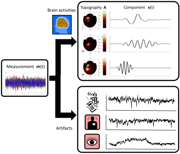
Figure 2.2: Independent Component Analysis. MEG/EEG signals are often corrupted by additive noises including background brain activities, heartbeat, eye-blinking, other elec-trical muscle activities and the environment noises. In general, these interferes occurs inde-pendently to the stimuli or ERFs. Recently, ICA has been proved a useful tool in analyzing MEG/EEG signals, especially for artifacts removal. It attempts to find the unmixing matrix W that makes the output components as independent as possible.

MEG/EEG signals are often corrupted by additive noises including background brain activities, heartbeat, eye-blinking, other electrical muscle activities and the environment noises (Figure 2.2). In general, these interferes occurs independently to the stimuli or event-related fields (ERFs).

(33)

2.4 Electromagnetic Spatiotemporal Independent Component Analysis

(EMSICA) 13

blind source separation to find components that are mutually statistical independent [21]. It performs best when raw or unaveraged signals are applied as inputs. Recently, it has been proved a useful tool in neurological brain research and is widely-used for analyzing MEG/EEG signals [18, 19], especially for removing the interferences mentioned above as a preprocessing step based on its independence assumption [4, 8, 17, 22]. Moreover, it may be probable to see the ERFs after removing noises and be helpful for the following source estimation process.

The ICA task is casted as follows:

m(t) = Ax(t) (2.8)

, A ∈ RN ∗K is so called a mixing matrix that compounds the K independent components x(t) ∈ RK_{into MEG measurement m(t). Each single column vector a}

iof mixing matrix A

is respected to the ithcomponent xi = [xi(t1) . . . xi(tT)], for i = 1 . . . K, which specifies

its distribution to MEG sensors. In contrast, the equation 2.8 can also be written as

WTm(t) = x(t) (2.9)

where W ∈ RN ∗K is the unmixing matrix. Each single column vector wi of unmixing

matrix W is a filter extracting the corresponding component xi from MEG measurement.

However, the amount of output independent components is limited to the number of input channels. That is, at most N components will be outputted if we send a N -channel MEG measurement to ICA.

2.4 Electromagnetic Spatiotemporal Independent

Compo-nent Analysis (EMSICA)

Electromagnetic Spatiotemporal Independent Component Analysis (EMSICA) was pro-posed by Arthur C. Tsai et al. in 2006 [33] for estimating spatiotemporal independent EEG components and the corresponding cortical source distribution. It is implemented using Bayesian statistical framework for imaging independent brain activities under physiologi-cal source constraints.

(34)

First, it assumes that P brain activities are consisted of the K spatiotemporal indepen-dent components and the matrix B ∈ P ∗ K describes the linear combination.

s(t) = Bx(t) (2.10)

Each column vector bi ,where B = [b1. . . bK] , represents the cortical distribution of

component xi(t) for i = 1 . . . P . Thus, the forward solution (Eq. 2.3) becomes

m(t) = Ls(t) = LBx(t). (2.11)

Topography

Cortical distribution Component

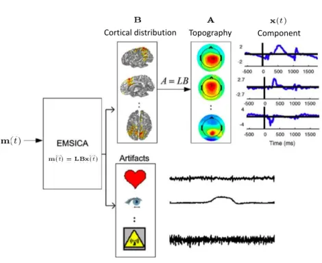
Figure 2.3: EMSICA.

(This picture is excerpted from [33])

EMSICA attempts to estimate the cortical distribution B that makes the corresponding output components as independent as possible. Moreover, compare equation 2.8 for ICA and 2.11, distribution of independent components to sensors are obtained by Equation 2.12. Thus, there are distributions to both cortical surface and sensor space.

(35)

2.5 Comparison between ICA and EMSICA 15

the corresponding output components as independent as possible and K, the amount of components, must be less than or equal to P or said the number of brain activities.

2.5 Comparison between ICA and EMSICA

EMSICA and ICA both attempt to extract independent components from input signals and to find the respected distribution. According to the Equation 2.8 from ICA and 2.11 from EMSICA, the relation between distribution to sensor space from ICA and to cortical surface from EMSICA can be illustrated by

A = LB. (2.12)

(a) (b)

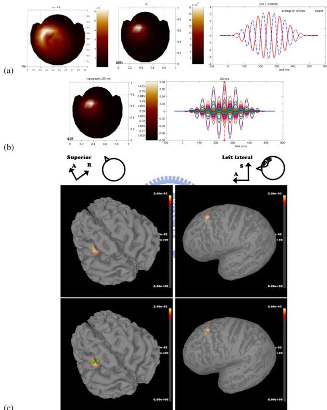
Figure 2.4: Infomax ICA in sensor space vs. EMSICA on cortical surface. (These two pictures are excerpted from [33])

(a) Topography with respect to 12 components, accounting for sensorimotor mu, frontal midline theta, central and lateral posterior alpha rhythms, separated using infomax ICA. (b) Cortical distribution of the 12 components extracted by EMSICA and the corresponding topography by applying lead field matrix to cortical distribution map. Results of EMSICA similar to the ones of ICA demonstrates that EMSICA has the convinced ability to separate components well like what the widely-used ICA has.

(36)

Figure 2.4 displays the results of a two-back visual memory working memory task an-alyzing by standard ICA and EMSICA. The topographies, outputted by ICA, displayed in left-panel and the ones, transformed from cortical distribution by lead field matrix, dis-played in right-panel are similar. This demonstrates that EMSICA has the convinced ability to separate components well like what the widely-used ICA has.

Moreover, EMSICA, within a single procedure, solves not only independent compo-nents but also the imaging of cortical source distribution by involving the forward solution and implemented using Bayesian framework. This makes the difference between ICA who is not an imaging method and just separates components in the same space as input signals. On the other hand, ICA can split components in cortical space as the second procedure but an imaging or inverse method to measurement required at first [35].

Comparing these two algorithms, EMSICA has the ability to estimate cortical source distribution but also has too many variables, at least 110,000 triangular points consisted of the cortical surface in our case, locations of dipolar sources need to be solved. In contrast, standard ICA cannot estimate cortical source distribution directly when applied measure-ment but not cortical sources. Furthermore, ICA has same accuracy in sensor space but handles the smaller data and fewer variables than EMSICA does.

(37)

Chapter 3 Spatiotemporal Imaging of Independent

Brain Activities

(38)

18 Spatiotemporal Imaging of Independent Brain Activities

Under the assumption, described in Section 2.4 by the forward solution (Equation. 2.11), brain activities s(t) are composed of numbers of spatiotemporal independent compo-nents x(t) with cortical distribution B. We propose a method for spatiotemporal imaging of independent components, estimated using standard ICA, by lead field vector space pro-jection. Thus, it has advantages of small data size and fewer variables like standard ICA but also has the ability to map independent components to cortical surface like EMSICA.

3.1 Mixing Matrix Approach for Imaging Method

According to equation 2.12, each mixing vector aihas its corresponding cortical

distri-bution bi. They can be explained to the distribution of a component to sensors and cortical

surface. Moreover, birepresents the linear combination of lead field vector that consists the

respective mixing vector. Thus, if mixing matrix A and lead field matrix L are given, the cortical source distribution can be solved by Equation 3.1 where L+ is solved by singular value decomposition.

B = L+A (3.1)

Since mixing matrix A are linearly combined from lead field matrix L by the combina-tion B, we apply SVD to L for finding a set of basis that well-represent the mixing matrix A. Therefore, the linear combination B is solvable when L+_{and A are known.}

However, according to the definition of ICA, unmixing matrix W is estimated at first for making the output components as independent as possible. Mixing matrix is calculated by Equation 3.2 from unmixing matrix W for representing the distribution of components to sensors. Because A is not real inverse of W, there must exist some distortion of A.

A = W+ (3.2)

Then, Equation 3.3 becomes Equation 3.3 but it remains in doubt. Both L+_{and A}+_are

distorted. There must be too much distortion of the output B. The effect were observed by simulation described in later chapter.

(39)

3.2 Unmixing Matrix Approach for Imaging Method 19

B = L+W+. (3.3)

Consider the definition of ICA, W seems more suitable for calculating the cortical source distribution and it is describe in next section.

3.2 Unmixing Matrix Approach for Imaging Method

The deduction starts from the forward equation 2.11 and assumes independent compo-nents spanning the whole signal space. By applying standard ICA to measurement to obtain the spatial filter or unmixing matrix W, the corresponding outputs x(t), representing the time course of independent components at time t, can be illustrated by equation 3.4.

WTm(t) = WTLBx(t) = x(t) (3.4)

Moreover, the column vector x(t) is an eigenvector of matrix C if we let C = WT_LB

and then Cx(t) = x(t). Based on the assumption that independent components x(t) span the whole signal space, C must be an indentity matrix such that WTLB is indentity. Thus, the cortical source distribution B can be solved by singular value decomposition (SVD) (Eq. 3.5).

B = (WL)+ (3.5)

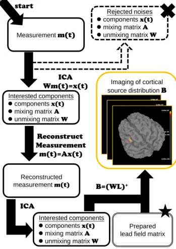
In summary, Figure 3.1 illustrates the work flow of the proposed method. Standard ICA is applied as a preprocessing procedure for picking features and removing uninterested brain activities or other interferes. And then, project the interested components by lead field to obtain the corresponding cortical source distribution.

Work Flow

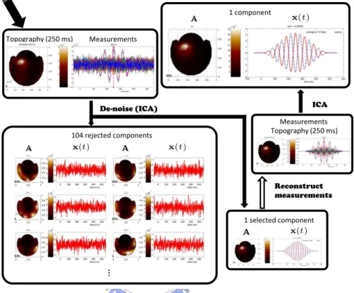
Figure 3.1 shows the work flow for spatiotemporal imaging of independent components. ICA is executed twice here. The first-stage ICA is for feature selection, or said reject the uninterested components and is regarded as a preprocess step. Thus, measurement should

(40)

20 Spatiotemporal Imaging of Independent Brain Activities

be reconstructed using Equation 2.8 whenever the rejection is done. And then, second-stage ICA is executed for separating independent components for imaging in later steps.

Moreover, the lead field is made up under physiological source constraints, that is lo-cation and orientation is segmented from the MR image. Thus, it can be pre-cauculated for each subject. Measurement m(t) start ICA Wm(t)=x(t) Interested components  components x(t)  mixing matrix A  unmixing matrix W Rejected noises  components x(t)  mixing matrix A  unmixing matrix W Reconstruct Measurement m(t)=Ax(t) Reconstructed measurement m(t) Interested components  components x(t)  mixing matrix A  unmixing matrix W Prepared lead field matrix

B=(WL)+

ICA

Imaging of cortical source distribution B

Figure 3.1: Work flow - lead field vector space projection for spatiotemporal imaging of Independent Brain Activities Standard ICA is applied as a preprocessing procedure for picking features and removing uninterested brain activities or other interferes. And then, project the interested components by lead field to obtain the corresponding cortical source distribution.

(41)

Chapter 4 Experiments

(42)

22 Experiments

For verifying the algorithm we proposed, we have done experiment of three simula-tions. These data were simulated with cortical surface constraints. Thus, in the first sec-tion, materials such as MR images, MEG instrument and cortical surface are described. The procedure of reconstructing cortical surface is consisted of three steps. It must be seg-mented by FreeSurfer, which is a set of software tools for study of cortical and subcortical anatomy, at first. Then, it is down sampled using VTK, which is a visualization toolkit and open source software for 3D computer graphics. Moreover, for easy observation of the cortical source distribution in sulcus, FreeSurfer is applied to inflate the down-sampled surface.

The first simulation is the simplest one that only one dipolar source was placed at a single position. Both the two approach using mixing and unmixing matrix were applied to the first simulation. Apparently, the unmixing matrix approach is much more accurate then mixing matrix approach. This is under our expectation. Thus, the imaging method must apply approach by unmixing matrix but the mixing matrix.

A tangent dipolar source is placed in simulation two for verify the accuracy of the imag-ing method since tangent should be separated better theoretically than sine when surround-ing by lots of sine interferes. Accordsurround-ing to the experiment result, it is perfectly mapped to cortical surface because it is separated better than sines placed in the same place of the other simulations.

In the last simulation, it becomes much more complicated that four sources were placed at three location. It means there are two sources in one place. Moreover, one of these two sources was placed elsewhere. Even in the hard condition, the imaging method still works fine. The more detail are described in the following sections.

4.1 Materials

4.1.1 3D MR Images

T1-weighted MR head images were acquired on a 1.5 Tesla GE MR scanner, using 3D-FSPGR pulse sequence (TR = 8.67 ms, TE = 1.86 ms, TI = 400 ms, NEX = 1, flip angle = 15◦, bandwidth = 15.63 kHz, matrix size = 256 × 256 × 124, voxel size = 1.02 × 1.02 × 1.5

(43)

4.1 Materials 23

(www.arts.uwaterloo.ca/~bfleming/psych261/)

Figure 4.1: Surface of Brain.

(This picture is excerpted from http://www.arts.uwaterloo.ca/ bfleming/psych261/)

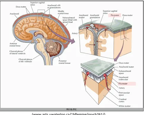
The two kinds of surfaces reconstructed by FreeSurfer are pia mater and white mater. Ac-cording to the physiological knowledge, pia mater closely envelopes the entire surface of the brain and is the closet one of these two reconstructed surface to the cortex. Thus, it is the picked physiological constraints of the proposed method for imaging of brain activities.

mm3).

4.1.2 Cortical Surface Reconstruction

Estimation of the proposed imaging method is based on physiological source con-straints that brain activities locate on cortical surface with orientations, or said the surface normal, perpendicular to the surface. On the other hand, the informations of cortical surface are the prior knowledge.

The cortical surface is segmented using FreeSurfer [9] which is a set of software tools for study of cortical and subcortical anatomy. FreeSurfer segments the 3D volume data, MR image, into two kinds of surface that are pia mater and white mater representing by

(44)

24 Experiments

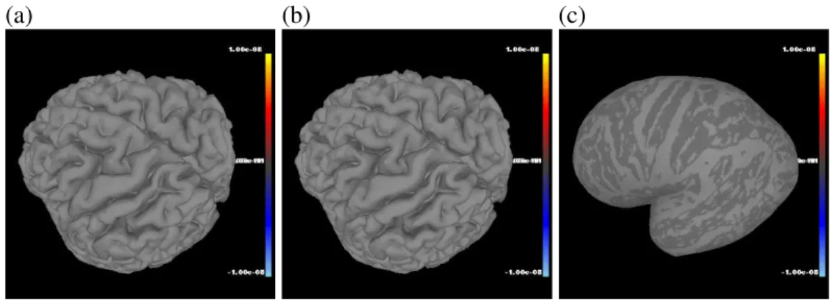
(a) (b) (c)

Figure 4.2: Reconstructed Pia Mater (a) Pia mater has been down sampled by 50% and 114,024 triangular points remain. (b) The original pia mater, composed of 228,044 tri-angular points, reconstructed by FreeSurfer. (c) The down sampled surface is inflated by FreeSurfer for clearly displaying the cortical source distribution. Gyrus is colored in gray and sulcus is colored in dark gray.

triangle meshes and each of them formed by a set of triangular points.

According to the physiological knowledge, electromagnetic fields are generate by a layer of pyramid cells in the cortex and pia mater is the closest one of the three kinds of brain surface outside the cortex, where the other ones are dura mater and arachnoid mater, to the cortex (Fig. 4.1). Hence, we pick the pia mater which closely envelopes the entire surface of the brain as the physiological constraint.

However, there are 228,044 points formed the triangle mesh of reconstructed pia mater (Fig. 4.2(b)). For easy calculation but with the tolerable distortion and non-smoothness, the pia mater surface is down sampled by 50% using VTK which is a visualization toolkit and open source software for 3D computer graphics. Thus, there are 114,024 points remained for our dipolar source imaging method (Fig. 4.2(a)). Moreover, the down sampled sur-face was inflated by FreeSurfer for displaying cortical sursur-face clearly, especially for sulcus colored in dark gray (Fig. 4.2(c)).

4.1.3 MEG Device

The simulations was generated according to the device information from a real MEG measurement. The measurement was acquired by a whole head MEG system ”Neuromag

(45)

4.2 Experiments 25

Vectorview 306” which belongs to Taipei Veterans General Hospital. The MEG system is placed in a magnetically shielded room and has the capability of 306 channels simultane-ously recording at 102 distinct sites, 24 bits analog to digital conversion, and up-to-8 kHz sampling rate which is sufficient to probe the fast dynamics inside human brain.

4.1.4 Data Preprocessing

For low SNR, it results from the much smaller scale of electrophysiological signal than of environmental noises. For instance, the magnitude of omnipresent static field of earth is around 10−1 Tesla and is much larger than of the induced magnetic field which is around 10−10 to 10−15 Tesla. In addition, MEG and EEG signals are often corrupted with the background brain activities and artifacts, such as the heartbeat, eye-blink, and environmen-tal noises. Thus, data preprocessing is required for noise reducing.

Independent Component Analysis (ICA) are some commonly adopted techniques for increasing the SNR or rejecting artifacts. ICA was originally proposed for the purpose of blind source separation to find components that are mutually statistical independent [20]. It performs best when raw or unaveraged signals are applied as inputs. Recently, it has been proved a useful tool in neurological brain research and is widely-used for analyzing MEG/EEG signals [17, 18], especially for removing artifacts based on its independence as-sumption [3, 7, 16, 21]. In the following experiments, the fisrt-stage ICA is applied for noises removal in both simulation and real data. Moreover, for selecting useful trials from real data, Signal-space-project (SSP) and EOG rejection is applied.

4.2 Experiments

As aforementioned in Section 2.2, simulation uses the forward solution with spherical head model. And according to the electrophysiological basis, the MEG/EEG sensors are most sensitive to the electromagnetic field with orientation that lying on the tangential plane of the spherical shell. Therefore, the dipolar sources in our simulations are placed at sulcus but not at gyrus and then the dipole orientations are almost tangential.

(46)

26 Experiments

said the background noises, with standard deviation 0.1 nAm within the sphere with radius of 7 cm and was simulated 10 trials in 1,001 sampling rate. Each trial was 1 second long. The analysis steps follow the work flow described in chapter 3 by Figure 3.1

The first simulation is the simplest case that a single sine dipolar source is placed. The second one places two dipolar sources, where one is a sine wave and the other is a tangent wave, at two distinct positions. ICA performs well in the first two simulations. The given dipolar sources are almost perfectly identified and the cortical distributions are agreeable to the ground truth.

In the last simulations, four dipolar sources are placed at three distinct positions where two of them are the same sine waves but differed in amplitudes and locations and the others are two sine waves with different frequencies located at two distinct places. ICA also performs well to identify three different time courses but one of them with additive leakage from another component. But even with the leakage, the proposed method still produces an agreeable imaging of cortical distributions.

The accuracy is examined by location error and similarity of temporal activities. Loca-tion error is represented by distance between locaLoca-tion of the peak of cortical source distribu-tion and of the ground truth. Similarity between the given sources and picked components is represented by correlation coefficient corr(xi, xj) = (xi· xj)/(kxikkxjk). The smaller

location error and the higher similarity it has, the more accurate it is.

4.2.1 Simulation 1 - A Single Sine Dipolar Source

Ground Truth

In the first simulation, Figure 4.4 shows the ground truth that a 15 Hz sine wave (4.4(c)) is placed at r1 = (−29.47, 49.14, 94.75) mm and oriented to q1 = (0.80, −0.10, 0.60) in

MEG head coordinates (4.4(a)). Figure 4.4(b) displays the respective lead field vector with parameter θ1 = {r1, q1}. Figure 4.3 is the simulated measurement and the distribution to

MEG sensors, so called a topography, at 250 ms which is the peak time. The distribution of measurements to sensors at peak time is similar to the given lead field and is agreeable to our expectation.

(47)

Figure 4.3: Simulation 1 - The Output Measurement and Topography at 250 ms

R A

(a)

(c) (b)

Figure 4.4: Simulation 1 - Ground Truth. (a) The location r and orienation q of the dipolar source are indicated by the blue arrow. In the right panel, (b) lead field vector of the source with parameter θ = {r, q} and (c) the 15 Hz sine wave are displayed.

(48)

28 Experiments

No. Method Similarity of Temporal Activities Location Error (mm)

1 (B = WL)+ _0.9954 _4.67

1’ B = L+A 0.9954 127.73

Table 4.1: Simulation 1 - Location Error and Similarity. The spatiotemporal imaging of the two interested components are almost perfectly fit the ground truth.

ICA result

There are 105 independent components extracted from input measurement by the first-stage ICA (Fig. 4.5). And then reconstruct measurement by 1 interested component, which is closely correlated to the given source for simulation, and the respective mixing vector. Finally, the second-stage ICA outputs 1 interested component and it is picked to be mapped to cortical surface.

Cortical Source Distribution

There is 1 component regarded as the given source (Fig. 4.7(a)) and the respective cortical distribution (Figure 4.7(c)) displayed in both cortical surface and the inflated sur-face of the left hemisphere. The two figures in the bottom with green arrow and point that indicate the ground truth. Consequently, the cortical distribution demonstrates that the picked component was activated around the highlighted area and the location of peak of this distribution is close to the ground truth at distance of 4.67 mm.

Here we verify the two approach solving cortical source distribution of the same com-ponent by mixing and unmixing matrix according to Equation 3.1 and 3.3. The results are displayed in Figure 4.7 and 4.8 with respect to the unmixing matrix approach and mixing matrix approach. Apparently, the later performs awful even that the ground truth had been found but the most activated region was far way from the ground truth with 127.73 mm location error (Table. 4.1).

(49)

4.2 Experiments 29 1 component 104 rejected components 1 selected component De-noise (ICA) Reconstruct measurements ICA Measurements Topography (250 ms) Topography (250 ms) Measurements …

Figure 4.5: Simulation 1 - ICA Decomposition.There are 105 components output but only 1 interested component according to the first-stage ICA.

Figure 4.6: Simulation 1 - the reconstructed measurement and topography by 1 se-lected ICA output components

(50)

30 Experiments (a) (b) (c) R A

Superior Left lateral

A S

Figure 4.7: Simulation 1 - Cortical Source Distribution Using Unmixing Matrix Ap-proach. (b) The interested component in red, closely correlated to the given source in blue, extracted by the 2nd-stage ICA and its topography. The left-most picture represents the reconstructed mixing vector ˜a1 = Lb1. (b) The measurement and topography at 250 ms

which is reconstructed by 1 component, extracted by the 1st-stage ICA, and the respective mixing vector (c) Cortical source distribution b1. The green arrow and point indicate the

(51)

R A

A S R A Inferior R S Posterior

Figure 4.8: Simulation 1 - Cortical Source Distribution Using Mixing Matrix Ap-proach. Cortical source distribution b10. The green arrow and point indicate the ground

truth. The region with strongest activation is located at inferior (the bottom two pictures) that is far away from the ground truth. Location of the peak of b10 and ground truth are at

(52)

32 Experiments (a) Location ri (mm) Orientation qi i x y z x y z 1 -29.47 49.14 94.75 0.80 -0.10 0.60 2 -34.90 -18.64 89.52 0.80 0.12 0.59 (c) Sources

No. Fig. 4.10 waveform location freq. (Hz) duration (ms) strength (nAm)

1 (b) tangent r1 11 0–500 1.0

2 (c) sine r2 15 0–500 1.0

Table 4.2: Simulation 2 - Ground Truth Two dipolar sources were placed at (a) two distinct locations and the distances between the two locations are listed in the right panel. (b) Table on the bottom lists information of dipolar sources including location, frequency, and duration. (See Fig. 4.10)

4.2.2 Simulation 2 - Two Uncorrealated Dipolar Sources

Ground Truth

Two uncorrelated dipolar sources, 11 Hz tangent and 15 Hz sine wave, were placed in the second simulation. The ground truth is listed in table 4.2 and displayed in Figure 4.10. The simulated measurement and topography for 250 ms is shown in Figure 4.9 which is similar the to the given lead field vector lθ2 (Figure 4.10(c)).

(53)

4.2 Experiments 33 (d) R A S (b) (c) (a)

Figure 4.10: Simulation 2 - Ground Truth. (a) Two kinds of sources. (b) 11 Hz tangent dipolar source and the respective lead field with parameter θ1 = {r1, q1} indicated by the

green arrow. (c) 15 Hz sine dipolar source and the respective lead fields with parameter θ2 = {r2, q2} indicated by the blue arrows. (d) Ground truth on cortical surface.

ICA result

There are 93 independent components extracted from input measurement by the first-stage ICA (Fig. 4.11). And then reconstruct measurement by 2 interested component, which are closely correlated to the given sources, and the respective mixing vector. Finally, the second-stage ICA outputs 2 component and they are picked to be mapped to cortical surface.

There are 2 components regarded as the given sources (Figure 4.12(a) and Figure 4.13(a)) and the respective cortical distribution (Figure 4.12(c) and Figure 4.13(c)) displayed in both cortical surface and the inflated surface of the left hemisphere. The two figures in the bottom with green arrow and point that indicate the ground truth. In this simulation, the spatiotemporal imaging of the two components are almost perfectly fit the ground truth with small location errors with location error less than 1 mm(Table 4.3).

(54)

34 Experiments 2 components 91 rejected components 2 selected components De-noise (ICA) Reconstruct measurements ICA Measurements Topography (250 ms) Topography (250 ms) Measurements

…

Figure 4.11: Simulation 2 - ICA Decomposition. There are 93 components output but only 2 interested component according to the first-stage ICA.

No. Wave Freq. (Hz) Similarity of Temporal Activities Location Error (mm)

1 tangent 11 0.9997 0.00

2 sine 15 0.9953 0.91

Table 4.3: Simulation 2 - Location Error and Similarity. The spatiotemporal imaging of the two interested components are almost perfectly fit the ground truth.

(55)

4.2 Experiments 35 (a) (b) (c) R A

A S

Figure 4.12: Simulation 2 - Cortical Distribution of the 1st component. (a) The out-put component and its topography is compared to the given tangent source. The left-most picture represents the reconstructed mixing vector ˜a1 = Lb1. (b) According to the

recon-structed measurement, topography for 227 ms which is the peak time the tangent source but with weaker activation of the other source. (c) According to the cortical distribution, the strongest activation of the tangent component is exactly located at the ground truth position.

(56)

36 Experiments (a) (b) (c) R A S Left lateral A S

Figure 4.13: Simulation 2 - Cortical Distribution of the 2nd component. (a) The output component and its topography is compared to the given sine source.The left-most pic-ture represents the reconstructed mixing vector ˜a2 = Lb2. (b) According to the

recon-structed measurement, topography for 250 ms which is the peak time the sine source but with weaker activation of the other source. (c) According to the cortical distribution, the strongest activation of the sine component is located around the ground truth position in distance of 0.91 mm.

(57)

4.2 Experiments 37 (a) Location ri(mm) Orientation qi i x y z x y z 1,3 -29.47 49.14 94.75 0.80 -0.10 0.60 2 -26.82 -0.36 105.64 0.83 0.45 0.34 4 23.63 35.00 98.09 0.94 0.08 -0.34 Distance kri− rjk i\j 2 4 1,3 50.75 50.90 2 63.32 (c) Sources (sine)

No. Figure 4.15 wave color location freq. (Hz) duration (ms) strength (nAm)

1 (b) green r1 7 0–500 0.3

2 (c) blue r2 17 50–350 0.5

3 (b) red r3=r1 31 0–200 0.7

4 (d) red r4 31 0–200 1.0

Table 4.4: Simulation 3 - Ground Truth Four dipolar sources were placed at (a) three distinct locations and the distances between the three locations are listed in the right panel. (b) Table on the bottom lists information of dipolar sources including location, frequency, and duration. (See Figure 4.15)

4.2.3 Simulation 3 - Four Sine Dipolar Sources

Ground Truth

In the third simulation, Figure 4.15 and Table 4.4 shows the ground truth that four dipolar sources are placed at three distinct positions which means two of the sources, the first and the third one, are at the same location.

In Figure 4.15, temporal activities and locations of the four dipolar sources are distin-guished by colors and locations are numbered. temporal activity of the first source, a 7 Hz sine wave with duration 0-200 ms, in green (Figure 4.15(b)) is located where the green arrow numbered in 1 indicates (e). Temporal activity of the second source, a 17 Hz sine wave with duration 50-350 ms, in blue (Figure 4.15(c)) is located where the blue arrow numbered in 2 indicates (Figure 4.15(e)).

Temporal activities of the third and the fourth source, 31 Hz sine waves with duration 0-200 ms but with different strength 0.7 and 1 nAm, in red numbered in 3 and 4

(58)

(Fig-38 Experiments

Figure 4.14: Simulation 3 - The Output Measurements and Topography. The simulated measurements contain 4 dipolar sources and 3000 random dipoles. The topography in 250 ms is displayed in the left panel and the peak is around the location of the given 17 Hz sine.

ure 4.15(c)) are located at two distinct positions. The weaker one is located at the same place as the 7 Hz sine in green and the stronger one is individually placed at location No. 3. The output measurements and topography in 250 ms are displayed in Figure 4.14.

ICA result

There are 105 independent components extracted from input measurement by the first-stage ICA (Figure 4.17). And then reconstruct measurement by 3 interested components (Figure 4.16), which is closely correlated to the given sources for simulation, and the re-spective mixing vectors. Finally, the second-stage ICA outputs 3 interested component and they are picked to be mapped to cortical surface.

See Figure 4.18 for more detail about the first component. There are three temporal activities plotted in the figure on top. The 1st output component is plotted with red solid line. The given 7 Hz sine is plotted with green dashed line. The similarity between temporal activities of the output component and the given 7 Hz sine is 0.9886. Look at the blue dashed line in figure on top, it represents the combination of 7 and 17 Hz sines, by 98.86% 7 Hz sine minus 10% 17 Hz sine, and its similarity between the component becomes higher to 0.9985. Apparently, this component is strongly correlated to 7 Hz sine but also receives a little leakage from 17 Hz sine at the later segment of temporal activity. In addition, the leakage effect can be observed from the mixing vector and lead field vector of the given 17 Hz sine, plotted in blue.

(59)

4.2 Experiments 39 (a) (b) (c) _(d) (e) 1 2 4 1 2 3 3 R A 4

Figure 4.15: Simulation 3 - Ground Truth. (a) Three kinds of dipolar sources. (b) 7 Hz and 31 Hz dipolar sources with duration 50-350 ms and 0-200 ms. Topography is the respective lead field. Location and orientation of the two sources are indicated by the arrow both in red and green numbered in 1 and 3. (c) A 17 Hz sine dipolar sources with duration 0-500 ms and the respective lead field where location and orientation are indicated by the blue arrow numbered in 2. (d) A 31 Hz sine dipolar source with duration 0-200 ms and the respective lead fields where location and orientation are indicated by the red arrow numbered in 4. Attention that this 31 Hz sine is almost the same as the red one in (a) except that 31 Hz sine has stronger activation on this position than on the first position. (e) Ground truth on cortical surface.

Figure 4.16: Simulation 3 - the reconstructed measurement and topography The mea-surements m(t) were reconstructed by 3 selected components x(t) the the respective mix-ing vectors A where m(t) = Ax(t). (See Figure 4.17)

(60)

40 Experiments 3 components ICA De-noise (ICA) Reconstruct measurements Measurements Topography (250 ms) 102 rejected components … 3 selected components Topography (250 ms) Measurements

Figure 4.17: Simulation 3 - ICA Decomposition. After the first-stage ICA, there are 105 components output but only 3 interested components that closely correlated to the given sources. The similarity of temporal activities of given sources and components are listed in Table 4.5

1stsource 2ndsource 1stcomponent

+ *0.9886 *-0.1000

Lead field Lead field

Figure 4.18: Simulation 3 - Leakage of the 2nd Component. There are three temporal activities plotted in the figure on top. The 1st output component is plotted with red solid line. The given 7 Hz sine is plotted with green dashed line. The similarity between temporal activities of the output component and the given 7 Hz sine is 0.9886. Look at the blue dashed line in figure on top, it represents the combination of 7 and 17 Hz sine sources, by 98.86% 7 Hz sine minus 10% 17 Hz sine, and its similarity between the component becomes higher to 0.9985. Apparently, this component is strongly correlated to 7 Hz sine but also receives a little leakage from 17 Hz sine at the later segment of temporal activity. In addition, the leakage effect can be observed from the mixing vector and lead field vector of the given 17 Hz sine, plotted in blue.

(61)

No. Sine (Hz) Similarity of Temporal Activities Location Error (mm)

1 7 and 17 0.9985 3.64 and 2.18

2 17 -0.9851 3.62

3 31 -0.9810 3.38 and 0.00

Table 4.5: Simulation 3 - Location Error of Cortical Source Distribution

There are 3 components (Figure 4.17) regarded as the given sources (Figure 4.15) and the respective cortical distribution (Figure 4.19–4.21) displayed in both cortical surface and the inflated surface of the left hemisphere.

It differs from the first two simulations that the first component shown in Figure 4.18 is not perfectly fit the given 7 Hz sine but also receives a little leakage from the 17 Hz sine. In addition, the leakage effect can also be observed from the corresponding mixing vector and the cortical distribution. In Figure 4.19, Cortical distribution of the 7 Hz sine, the main element of the first component, shows that it is activated around the left frontal, the ground truth. And 17 Hz, the other element, is activated around the left posterior met the ground truth in the distance of 4.67 mm.

Cortical source distribution of the second component, meets the given 17 Hz sine, is displayed in Figure 4.20. The 17 Hz sine was placed at a single position and the strongest activation of cortical distribution is around the location of the ground truth in the distance of 2.17 mm.

Unfortunately, the location error of the peak of cortical source distribution of the third component, meets the given 31 Hz sine, is 16.33 mm that much larger than the other com-ponents and the peak is located across the gyrus from the ground truth (Figure ??). This phenomenon is going to be discussed in the next chapter.

(62)

42 Experiments (a) (b) (c) R A

A S

Figure 4.19: Simulation 3 - Cortical Distribution of the 1st component. (a) The output component and its topography is compared to the given sources. The left-most picture represents the reconstructed mixing vector ˜a1 = Lb1. (b) Cortical distribution with strong

activation at both ground truth location of 7 Hz near left frontal and 17 Hz sines in left posterior. Location of cortical distribution peak and the given 7 Hz sine is at distance of 3.64. Location of cortical distribution peak and the given 17 Hz sine is at distance of 2.18 mm.

(63)

4.2 Experiments 43 (a) (b) (c) R A

A S

Figure 4.20: Simulation 3 - Cortical Distribution of the 3rd component. (a) The output component and its topography is compared to the given sources. The left-most picture represents the reconstructed mixing vector ˜a2 = Lb2. (b) Cortical distribution with strong

activation around the ground truth location of 17 Hz sine in left posterior. Location of cortical distribution peak and the ground truth are at distance of 3.62 mm.

(64)

44 Experiments (a) (b) (c) Left lateral A S Right lateral A S Right lateral A S

Figure 4.21: Simulation 3 - Cortical Distribution of the 2nd component. (a) The output component and its topography is compared to the given sources. The left-most picture represents the reconstructed mixing vector ˜a3 = Lb3. (b) Cortical distribution with strong

activation around the ground truth location of 31 Hz sine in right hemisphere. Location of cortical distribution peak and the ground truth are at distance of 3.38 and 0.00 mm.

(65)

4.2.4 Experiments of Gender Discrimination

We propose the method for imaging of independent components extracted using the standard ICA algorithms. Even thought this method is neither for solving the inverse prob-lem nor for more precisely decomposing independent component, but it has proved to be helpful and provides a both intuitive and efficient solution for mapping the discovered fea-tures or interested components of MEG/EEG signals to cortical surface. Consequently, the discovered features can be directly mapped to cortical surface without redo the experi-ments.

In this section, the experiment result and cortical source distributions are calculated from the real recordings. Bipolar Disorder (BD) patients and normal subjects were asked to specify the genders of presented faces that prevents the subject’s explicit recognition or categorization of the emotion expressed. In the following subsections, the more detail of experiment paradigm will be described and we demonstrated the experiment result that calculated from the recording of angry condition of one normal subject.

Experiment Paradigm of Gender Discrimination

Twenty normal subjects and twelve bipolar disorder patients participate this experiment. Face images are gray-scaled photographs of faces, depicting neutral, angry, happy and sad. The task is to specify the gender of the presented faces that prevents the subject’s explicit recognition or categorization of the emotion expressed. Subjects are instructed to lift the right or left index finger while recognizing the presented face image as female or male. For each condition, about 288 trials, 20 minutes are retrieved. The experiment paradigm is shown in Figure 4.22. Each stimulus is separated in 3000 ms by the sign of plus. First, one image of emotional face is displayed for 1500 ms. The following is 1000 ms blank. Then, a cue to ask subjects to response for male or female by image of the question mark for 500 ms.

ICA Result and Preprocessing

We analyze the recordings of angry condition of one normal subject that there are 60 trials and the duration of each trial is from 0 to 500 ms. The sampling rate is 1001 Hz

(66)

46 Experiments sad sad happy happy angry angry 3000 ms 1500ms ~1000 ms 500 ms

face blank response cue

neutral

neutral _Male/Female?

Figure 4.22: Experiment Paradigm of Gender Discrimination. The task is to specify the gender of the presented faces that prevents the subject’s explicit recognition or categoriza-tion of the emocategoriza-tion expressed. Subjects are instructed to lift the right or left index finger while recognizing the presented face image as female or male. For each condition, neutral, happy, angry and sad, 20 minutes about 288 trials are retrieved. Each stimulus is separated in 3000 ms by the sign of plus. First, one image of emotional face is displayed for 1500 ms. The following is 1000 ms blank. Then, a cue to ask subjects to response for male or female by image of the question mark for 500 ms.

and thus there are 500 sample points of each trial. The flow-chart and result of ICA and preprocessing are shown in Figure 4.23 that all temporal activities are averaged out for 60 trials and plotted with duration of 0 to 200 ms except the top two pictures are plotted with duration of 0 to 500 ms. By the first-stage ICA as a de-noise step, there are 193 independent components extracted from input measurement. Then, reject 154 components by kurtosis value v ∈ R193 of each component [3] and thus 39 components remain. Components are rejected if kvi − vmeank ≥ 1.7 × vstd where vi is the kurtosis value of the ith component,

vmean is mean of v and vstd is the standard deviation of v. The number of output

compo-nents in second-stage ICA is also 39. Moreover, preprocessing steps, like band-pass filter and baseline correction, are applied to temporal activities of all 39 components. The pass band is from 2 to 50 Hz. Mean values of temporal activities during 350 to 450 ms, indi-cated by with red frame of the image on left-top side (Figure 4.23), are used for baseline correction. Then, these preprocessed components are all mapped to cortical surface.

(67)

4.2 Experiments 47 Measurements Topography (70 ms) 154 rejected components … 39 selected components … De-noise (ICA and kurtosis) Reconstruct measurements ICA

39 components

…

Band -pass filter: 2 – 50 Hz

Baseline correction: 350 – 450 ms … Temporal activities of all 39 components Temporal activities of all 39 components 39 components Measurements Topography (70 ms)

Figure 4.23: ICA Result of Real Data. We analyze the recordings of angry condition of one normal subject that there are 60 trials and the duration of each trial is from 0 to 500 ms. The sampling rate is 1001 Hz and thus there are 500 sample points of each trial. This figure shows the flow-chart and result of ICA and preprocessing that all temporal activities are av-eraged out for 60 trials and plotted with duration of 0 to 200 ms except the top two pictures are plotted with duration of 0 to 500 ms. There are 193 independent components extracted from input measurement by the first-stage ICA. Then, 154 components are rejected using kurtosis and 39 components remain. Moreover, preprocessing steps, like band-pass filter and baseline correction, are applied to temporal activities of all 39 components. The pass band is from 2 to 50 Hz. Mean values of temporal activities during 350 to 450 ms, indicated by with red frame of the image on left-top side, are used for baseline correction.

利用導場向量空間投影進行腦部獨立活動訊號源之時空造影

國

立

交

通

大

學

資訊科學與工程研究所

碩

碩

碩

碩

士

士

士

士

論

論

論

論

文

文

文

文

利

用

導

場

向

量

空

間

投

影

進 行 腦 部 獨 立 活 動 訊 號 源 之 時 空 造 影

Lead Field Vector Space Projection for Spatiotemporal

Imaging of Independent Brain Activities

研 究 生：陳姿樺

指導教授：陳永昇 博士

中

中

中

中 華

華

華 民

華

民

民 國

民

國

國

國 九

九

九

九 十

十 七

十

十

七

七

七 年

年

年 八

年

八

八

八 月

月

月

月

利用導場向量空間投影進行腦部獨立活動訊號源之時空造影

Lead Field Vector Space Projection for Spatiotemporal Imaging

of Independent Brain Activities

研 究 生：陳姿樺 Student：Tzu-Hua Chen

指導教授：陳永昇 Advisor：Yong-Sheng Chen

國 立 交 通 大 學

資 訊 科 學 與 工 程 研 究 所

碩 士 論 文

Contents

List of Figures

進行腦部獨立活動訊號源之時空造影

研究生：陳姿樺

指導教授：陳永昇博士

中華

_{華民}

_{民國}

_{國九}

_{九十}

_{十七}

_{七年}

_{年八}

_{八月}

_月

研究生：陳姿樺 Student：Tzu-Hua Chen

國立交通大學

資訊科學與工程研究所

碩士論文